Apr 25, 2007 - Robust Message-Passing for Statistical Inference in. Sensor Networks. Jeremy Schiff, Dominic Antonelli, Alexandros G. Dimakis,. David Chu ...
Robust Message-Passing for Statistical Inference in Sensor Networks Jeremy Schiff, Dominic Antonelli, Alexandros G. Dimakis, David Chu, Martin J. Wainwright Department of Electrical Engineering and Computer Science University of California, Berkeley, CA 94704 {jschiff,
dantonel, adim, davidchu, wainwrig}@eecs.berkeley.edu
ABSTRACT
1.
INTRODUCTION
Recent advances in hardware and software are leading to sensor network applications with increasingly large numbers of motes. In such large-scale deployments, the straightforward approach of routing all data to a common base station
Permission to make digital or hard copies of all or part of this work for personal or classroom use is granted without fee provided that copies are not made or distributed for profit or commercial advantage and that copies bear this notice and the full citation on the first page. To copy otherwise, to republish, to post on servers or to redistribute to lists, requires prior specific permission and/or a fee. IPSN’07, April 25-27, 2007, Cambridge, Massachusetts, USA. Copyright 2007 ACM 978-1-59593-638-7/07/0004 ...$5.00.
1
0.8 Relative Error
Large-scale sensor network applications require in-network processing and data fusion to compute statistically relevant summaries of the sensed measurements. This paper studies distributed message-passing algorithms, in which neighboring nodes in the network pass local information relevant to a global computation, for performing statistical inference. We focus on the class of reweighted belief propagation (RBP) algorithms, which includes as special cases the standard sum-product and max-product algorithms for general networks with cycles, but in contrast to standard algorithms has attractive theoretical properties (uniqueness of fixed points, convergence, and robustness). Our main contribution is to design and implement a practical and modular architecture for implementing RBP algorithms in real networks. In addition, we show how intelligent scheduling of RBP messages can be used to minimize communication between motes and prolong the lifetime of the network. Our simulation and Mica2 mote deployment indicate that the proposed algorithms achieve accurate results despite realworld problems such as dying motes, dead and asymmetric links, and dropped messages. Overall, the class of RBP provides provides an ideal fit for sensor networks due to their distributed nature, requiring only local knowledge and coordination, and little requirements on other services such as reliable transmission. Categories and Subject Descriptors: G.3 [Probability and Statistics]: Probabilistic Algorithms General Terms: Algorithms Keywords: Message-Passing Algorithms, Sensor Networks, Statistical Inference, Reweighted Belief Propagation
0.6
0.4
Reweighted BP Regular BP
0.2
0 0
20
40 60 Iterations
80
100
Figure 1. Graph of error versus iteration number for message-passing on a 9 × 9 nearest-neighbor grid. Standard belief propagation (BP, green curve) vs. reweighted belief propagation (RBP, blue curve).
may no longer be feasible. Moreover, such an aggregation strategy—even when feasible—can be wasteful, since it ignores which aspects of the data are relevant (or irrelevant) to addressing a given query. Consequently, an important research challenge is the development and practical implementation of distributed algorithms for performing data fusion in an in-network manner, thereby leading to useful statistical summaries of sensed measurements [22, 1]. Various problems that arise in sensor network applications, ranging from estimation and regression (e.g., predicting a “smoothed” version of a temperature gradient) to hypothesis testing (e.g., determining whether or not a fire has occurred), are particular instances of statistical inference. Past work on sensor networks [2, 1, 3, 10, 13, 14] has established the utility of formulating such inference problems in terms of Markov random fields, a type of graphical model in which vertices represent variables of interest and edges correspond to correlations between them. Moreover, given such a graphical model, it is possible to define simple messagepassing algorithms for performing inference, in which any given node passes “messages” to its neighbors that represent statistical summaries of local information relevant to a global computation. In a sensor network scenario, each mote is assigned a subset of variables of the Markov random field and we use the distributed wireless network of motes to exe-
cute the message-passing algorithm. The fact that message passing algorithms for graphical models require no global coordination translates to very simple and robust message passing algorithms for the sensor motes. The mapping of the graphical model to sensor motes and related issues are discussed in subsequent sections.
1.1
Related work and our contributions
It is well known that statistical inference for graphical models is computationally intractable in general (either an NP-hard or P# problem), but can be performed in exponential time using the junction tree algorithm. Paskin et al. [14] developed and implemented a robust architecture for the junction tree algorithm, suitable for performing exact inference in sensor networks. However, for many realistic networks (like grids or grid-like topologies) that have multiple cycles, the complexity of the junction tree method scales exponentially in the number of nodes, so that exact inference quickly becomes intractable. In such settings where exact inference is computationally intractable, message-passing algorithms 1 correspond to approximation schemes, which for a fixed number of iterations, the number of messages is linear in the number of edges of the graphical model. The BP algorithm, which is exact when applied to trees, has also been shown to frequently provide excellent approximations when applied to networks with cycles. It has been studied by various researchers [2, 3, 13, 10] for sensor network applications. The recent survey paper by Cetin et al. [1] (and references therein) provides further discussion of the issues that arise with graphical models and messagepassing in sensor networks. In contrast to previous work, this paper focuses on the class of reweighted belief propagation (RBP) algorithms, a larger family of algorithms which includes as special cases the standard BP and max-product algorithms for general networks with cycles. It is an attractive class from the theoretical perspective: in particular, certain RBP algorithms (different algorithms from standard BP) have guarantees of fixed point uniqueness, convergence, and robustness to message errors (for reweighted belief propagation [17, 15]), and correctness as well as convergence guarantees (for reweighted max-product [7, 20, 18]). These properties are not shared by the standard BP algorithm for general networks. Indeed, as illustrated in Figure 1, for certain network structures, the standard BP algorithm can yield highly inaccurate and unstable solutions to inference problems. In contrast to this instability, appropriately designed RBP algorithms are theoretically guaranteed to be robust to both message errors, and model mis-specification. A central thrust of this paper is that such issues of stability and robustness are of paramount importance in sensor network applications. Randomized message-passing algorithms for sensor networks have been explored for creating redundant representations of sensor data [4] and computing global functions of measurements in a distributed way [5]. For statistical inference, a number of researchers [3, 13, 10] have studied the use 1
Message-passing or belief propagation, when executed on graphs with cycles, is often called “loopy” belief propagation. There are different variants of belief propagation, including the sum-product updates for approximate marginalization, and the max-product updates for approximate maximization. The collective family of algorithms are jointly referred to as message-passing algorithms.
of standard BP for sensor networks at both the theoretical and simulation level. However, the work described here is (to the best of our knowledge) the first to actually implement a class of loopy message-passing algorithms—including BP as one exemplar—for sensor motes. More specifically, we design and implement an architecture for implementing RBP algorithms in real sensor networks. Our design does not rely on infrastructure such as reliable messaging, time synchronization and routing. We present simulation results evaluating algorithm performance under the real-world problems of failing motes and communication problems of failing links, asymmetric links, and dropped messages. We also show that intelligent scheduling, with greater communication between nodes on the same mote than nodes across motes, can make the algorithms converge with much less communication. We present experimental results from a prototype implementation using Mica2 motes. Our nesC implementation is modular and can be easily adapted for any message passing algorithm and scheduling policy, which as we show, is useful for numerous applications.
2.
BACKGROUND
We begin by providing background on graphical models, and then turn to discuss message-passing algorithms, including the standard and reweighted sum- and max-product algorithms.
2.1
Graphical models
We focus here on Markov random field (MRF) models, which are defined in terms of an undirected graph G, with vertex set V = {1, . . . , n} and edge set E. Associated with each node s ∈ V is a random variable Xs , representing (for our purposes) some type of sensor measurement or a quantity of interest, such as temperature in a particular location, which takes values either in some continuous space (e.g., X = R) or a discrete space (e.g., X = {0, 1, . . . , m − 1}). The structure of the graph G constrains the nature of the statistical interactions among the collection of random vari~ = (X1 , . . . , Xn ); in particular, we associate with ables X each vertex s a function ψs : X → R+ (called single-site compatibility function), and with each edge (s, t) a function ψst : X × X → R+ (called edgewise compatibility function). ~ Under the MRF asssumption, the joint distribution of X factorizes as Y 1 Y ψs (Xs ) ψst (xs , xt ), (1) p(~ x) = Z s∈V (s,t)∈E
i Q where Z = ~x∈X n s∈V ψs (Xs ) (s,t)∈E ψst (xs , xt ) is a normalization factor. Although it can be convenient to also define compatibility functions on larger subsets |S| > 2 of nodes, there is no loss of generality in making the pairwise assumption (1). P
2.2
hQ
Statistical inference in MRFs
Given an MRF of the form (1), it is frequently of interest to compute marginal probabilities at a particular node (or over some subset of nodes). Such marginalization problem involves summing over (subsets of) configurations, to determine for example, the marginal probability distribution of the temperature at some location given (possibly noisy) measurements at other locations. This problem is computationally challenging because the number of terms
in the summation grows exponentially in the size of the network (more specifically, we have |X n | = mn for a discrete MRF). A related problem is that of maximum a posteriori or MAP estimation: computing the most likely configuration given some observed data. For graphs with special structure—in particular, trees and more generally graphs of bounded treewidth2 —both the marginalization and MAP problems can be solved exactly with the junction tree algorithm [8], albeit with exponential complexity in treewidth. Many graphs commonly used to model sensor networks, including grid-based graphs and random geometric graphs, have unbounded treewidth, so that approximate algorithms are needed in practice.
2.3
Message-passing algorithms
In message-passing algorithms for graphical models, each node s in the MRF performs a local computation, and then transmits a summary to each of its graph neighbors. The message from node s to its neighbor t ∈ N (s) is a vector Mst (xt ), representing information that node t requires to perform the next round of computation. The sum-product form of message-passing is designed to solve the marginalization problem, whereas the max-product algorithm applies to the MAP problem. For tree-structured graphs (and with modifications for junction trees), both forms of these message-passing algorithms are guaranteed to be exact. The same updates are widely applied to general graphs with cycles, in which case they provide approximate solutions to inference problems. Here we first describe the family of reweighted belief propagation (RBP) algorithms, and then illustrate how a particular choice of edge weights yields the standard belief propagation algorithm. Various researchers have studied and used such reweighted algorithms for the sum-product updates [9, 17], generalized sum-product [19], and max-product updates [18, 7, 12, 20]. Each algorithm in this family is specified by a vector ρ ~ = {ρ, (s, t) ∈ E} of edge weights. The choice ρst = 1 for all edges (s, t) ∈ E corresponds to standard belief propagation; different choices of ρ ~ yield distinct algorithms with convergence, uniqueness, and correctness guarantees [17, 18]. For any fixed set of edge weights ρ ~, the associated reweighted BP algorithm begins by initializing all of the messages Mst to constant vectors; the algorithm then operates by updating the message along each edge according to the recursion Q [Mus (xs )]ρus X 1 u∈N (s)\t . Mst (xt ) ← ψs (xs ) [ψst (xs , xt )] ρst [Mts (xs )]1−ρst xs (2) These updates are repeated until the vector of messages ~ = {Mst , Mts | (s, t) ∈ E} converge to some fixed vecM ~ ∗ . The order in which the messages are updated is a tor M design parameter, and various schedules (e.g., parallel, treebased updates, etc.) exist. Upon convergence, the message ~ ∗ can be used to compute approximations to fixed point M the marginal distributions at each node and edge via Y qs (xs ) ∝ ψs (xs ) [Mts (xs )]ρst , (3) t∈N (s) 2
In loose terms, a graph of bounded treewidth is one which consists of a tree over clusters of nodes; see the paper [8] for further details.
and also to generate an approximation to the normalization constant. The update (2) corresponds P to the sum-product algorithm; replacing the summation xs by the maximization maxxs yields the reweighted form of the max-product algorithm. For the special setting of unity edge weights ρ = 1, the update equation (2) corresponds to the standard belief propagation algorithm. For any tree-structured graph, this algorithm is exact, and can be derived as a parallel form of dynamic programming on trees. On graphs with cycles, neither standard belief propagation (nor its reweighted variants) are exact. In this context, one useful interpretation of belief propagation is as a Lagrangian method for solving the so-called Bethe variational problem (see [21] for more details).
2.4
Algorithmic stability and robustness
In the case of standard BP (ρst = 1 for all edges (s, t)), there can be many fixed point solutions for the updates (2), and the final solution can depend heavily on the initialization. In contrast, for suitable settings of the weights [17] different from ρst = 1, the updates are guaranteed to have a unique fixed point for any network topology and choice of compatibility functions. Moreover, such reweighted BP algorithms are known to be globally Lipschitz stable in the following sense [17]. Suppose that q(ψ) denotes the approximate marginals when a RBP algorithm is used for approximate inference with data (compatibility functions) ψ. Then there is a global constant L, depending only on the MRF topology, such that kq(ψ) − q(ψ 0 )k ≤ Lkψ − ψ 0 k, where k · k denotes any norm. In loose terms, this condition guarantees that bounded changes to input yield bounded output changes, which is clearly desirable when applying an algorithm to statistical data. For special choices of compatibility functions (but not all choices), the standard BP updates are also known to be stable in this sense [16, 6]. Our experimental results described in Section 5 confirm the desirability of such stability.
3.
PROPOSED ARCHITECTURE
In the following section, we present StatSense, an architecture for implementing RBP algorithms in sensor networks. Our primary focus is the challenges that arise in implementing message-passing algorithms over unreliable networks with severe communication and coordination constraints.
3.1
Mapping from graphical models to motes
As described in Section 2, any Markov random field (MRF) consists of a collection of nodes, each representing some type of random variable, joined by edges that represent statistical correlations among these random variables. Any sensor network can also be associated with a type of communication graph, which in general may be different than the MRF graph, in which each vertex represents a mote and the links between motes represent communication links. As we discuss here, there are various issues associated with the mapping between the MRF graph and the sensor network graph [1]. For sensor network applications, some MRF random variables will be associated with measurements, whereas other variables might be hidden random variables (e.g., temperature at a room location without any sensor, or an indicator variables for the event “Room is on fire”). Any observable
result guarantees that it is always possible to modify the MRF so that this property holds: Proposition 1. Given any MRF model and connected mote communication graph, it is always possible to define an extended MRF, which when mapped onto the same mote communication graph, satisfies the no-routing property, and that message-passing on the mote communication graph yields equivalent inference solutions to the original problem.
Figure 2. Illustration of the two layers of the graphical model (left-hand subplot) and motes (right-hand subplot) used for simulation. Each node in the graphical model is mapped to exactly one mote, whereas each mote contains some number (typically more than one) of nodes. The red angle-slashed dots denote observation nodes (i.e., locations with sensor readings).
node may be associated with multiple measurements, which can be summarized in the form of a histogram representing a probability distribution over the data. In this context, the role of message-passing is to incorporate this partial information in order to make inferences about hidden variables. We assume that each node s in the MRF is mapped to a unique mote Γ(s) in the sensor network; conversely, each mote A is assigned some subset Λ(A) of MRF nodes. For any node s ∈ Λ(A), the mote A is responsible for handling all of its computation and communication with other nodes t in the MRF neighborhood N (s). Each node t ∈ N (s) might be mapped either to a different mote (requiring communication across motes) or to the same mote (requiring no communcation). Figure 2 illustrates one example assignment for a sensor network with 81 motes, and an MRF with 729 nodes. For instance, in this example, mote A is assigned nodes 1,2,3,26,27,28, 55, 56 and 57, so that Λ(A) = {1, 2, 3, 26, 27, 28, 55, 56, 57}, and Γ(1) = A etc. The sensor associated with each mote corresponds to an evidence node in the MRF; for instance, {1, 4, . . . , 82, . . . , 673} are evidence nodes in this example and we represent them as hashed nodes in Figure 2. Similar to previous work [11, 14], we assume a semi-static topology in creating the mote communication graph, so that we place an edge in this graph if there is a high-quality wireless communication link between these two motes. Note that the assignment of MRF nodes to motes may have a substantial impact on communication costs, since only the messages between nodes assigned to different motes need be transmitted. There is an additional issue associated with the node-mote assignment: in particular, the following property is necessary to preserve the distributed nature of message-passing when implemented on the sensor network link graph: for any pair (s, t) of nodes joined by the edge in the MRF, we require that the associated motes Γ(s) and Γ(t) are either the same (Γ(s) = Γ(t)), or are joined by an edge in the mote communication graph. We refer to this as the norouting property, since it guarantees that message-passing on the MRF can be implemented in motes with only nearestneighbor mote communication, and hence no routing. Thus, for a given MRF and mote communication graph, a question of interest is whether the no-routing property holds, or can be made to hold. It is straightforward to construct MRFs and mote graphs for which it fails. However, the following
Proof. Our proof is constructive in nature, based on a sequence of additions of nodes to the MRF model such that: (a) the final extended model satisfies the no-routing property, and (b) running message-passing on the mote communication graph yields identical inferences to message-passing with routing in the original model. Throughout the proof, the set of motes A, B, C, . . . and the associated mote communication graph remains fixed. The number of nodes and compatibility functions in the MRF as well as the mapping from nodes to motes are quantities that vary. Given any MRF model with variables (X1 , . . . , Xn ) and mote assignments (Γ(1), . . . , Γ(n)), suppose that the no-routing property fails for some pair (s, t), meaning that pair of motes Γ(s) and Γ(t) are distinct, and not joined directly by an edge in the mote link graph. Since the mote communication graph is connected, we can find some path P = {Γ(s), A2 , . . . , Ap−1 , Γ(t)} in the mote communication graph that joins Γ(s) and Γ(t). Now for each mote Ai , i = 2, . . . (p − 1), we add a new random variable Yi to the original MRF; each random variable Yi is mapped to mote Ai (i.e., Γ(Yi ) = Ai )). Moreover, let us remove the compatibility function ψst (xs , xt ) from the MRF factorization (1), and add to it the following compatibility functions ψes 2 (xs , y2 )
= ψek (k+1) (yk , yk+1 ) = ψe(p−1) t (yp−1 , xt ) =
I [xs = y2 ] I [yk = yk+1 ] ,
for k = 2, . . . , (p − 2).
ψst (yp−1 , xt ).
Here the function I(a, b) is an indicator for the event that {a = b}. The basic idea is that the variables (Y2 , . . . , Yp−2 ) represent duplicated copies of Xs that are used to set up a communication route between node s and t. By construction, the communication associated with each of the new compatibility functions ψe can be carried out in the mote graph without routing. Moreover, the new MRF has no factor ψst (xs , xt ) that directly couples Xs to Xt , so that edge (s, t) no longer violates the no-routing property. To complete the proof, we need to verify that when messagepassing is applied in the mote graph associated with the new MRF, we obtain the same inferences upon convergence (for the relevant variables (X1 , . . . , Xn )) as the original model. This can be established by noting that the indicator functions I collapse under summation/maximization operations, so that the set of message-fixed points for the new model are equivalent to those of the original model. Thus, we have shown that an edge (s, t) which fails the no-routing property can be disposed of, without introducing any additional links. The proof is completed by applying this procedure recursively to each troublesome MRF pair (s, t). Note that while one can design MRF models and corresponding communication graphs that contain a quadratic number of problematic edges, in practically interesting mod-
els, this transformation will only be rarely required, as discussed in Section 6.
3.2
Message updating
As mentioned previously, the message update scheme is a design parameter. The most common message update scheme is one in which all nodes update and communicate their messages at every time step according to (2), and proceed synchronously to new iterations. We term this scheme SyncAllTalk. Unfortunately, several factors discourage the direct application of SyncAllTalk to sensor networks. First, radio transmission and reception on embedded hardware devices consume nontrivial amounts of energy. Passing messages inter-mote is expensive and may overburden the already resource-constrained network. On the other hand, passing messages intra-mote incurs no significant energy cost because it is entirely local. This dichotomy indicates that we should limit messaging across motes when possible. Second, the SyncAllTalk protocol relies on synchronous message passing that inherently exhibits “bursty” communication patterns. For shared communication channels such as wireless, burstiness results in issues such as the hidden terminal problem, which further exacerbates the cost of radio transmission and reception. Last, for many situations, we expect sensor informativeness to vary greatly. For example, in a building monitoring scenario, the first sensor to detect a fire will generate much more informative messages than other sensors. Other scenarios have also resulted in similar observations [14]. Thus, evidence nodes, which often correspond directly to sensors, vary greatly in informativeness. We would like to favor more informative messages and thereby accelerate the rate of convergence. We have investigated a number of schemes which take advantage of these factors. The first scheme, SyncConstProb, exchanges all intra-mote messages at each time step as before, but only exchanges each inter-mote message with probability p at each time step. This means there is a direct decrease in the average period of inter-mote message transmission from once every time step to once every 1/p time steps. This scheme can trade convergence time for communication overhead. Probabilistic sending also reduces the burstiness that causes the hidden terminal problem. We can further decrease burstiness by relaxing the global time constraint. Instead, each mote proceeds at its own local start time and clock rate. As an additional benefit, this scheme does not rely on any time synchronization service. We refer to this scheme as AsyncConstProb. Our last scheme, AsyncSmartProb, makes the message transmission probability proportional to the informativenss of the message. Rather than reference a global constant probability of sending, p, each host sends with probability determined by some measure of distance between the old and new messages (cf. [1] for related ideas). One possible metric that we explore here is total variation distance raised to power η between the old and new messages: !η 1X 0 0 |Mst (xt ) − Mst (xt )| ∈ [0, 1]. (4) psend (Mst )= 2 x t
0 Here Mst denotes a new message that we may want to send from node s to node t, Mst denotes the previously sent message from node s to node t and η is a tunable “politeness”
factor. Note that if η ≈ 0, then p ≈ 1 so that messages are almost always sent, whereas for very large η, only the most informative messages have a substantial probability of being transmitted. All of the message passing schemes we investigate are extremely simple to implement, requiring no additional service infrastructure and operating exclusively with local computation. The traditional BP literature has proposed more sophisticated schemes in which all nodes exchange messages along graph overlays in organized sequence e.g. from the root of the overlay breadth-first. Unfortunately, these schemes typically require global coordination and are thus not as readily applicable in a sensor network context.
3.3
Handling communication failure
In general, when adapting algorithms to run on sensor networks, one must deal with network problems such as unreliable or asymmetric network links and mote failure. In the case of RBP, however, little adaptation is required. When a mote fails, the system simply ends up solving a perturbed inference problem on a reduced graphical model with all the nodes that belonged to that mote removed. If a network link fails, the resulting computation is equivalent to removing the corresponding edges from the graphical model. For both the case of mote and edge removals, we find empirically that the resulting increase in inference error remains localized near the removed nodes (or edges). The boundedness and localization of the error is again consistent with theoretical results on the Lipschitz stability of RBP algorithms [17, 15] (see also Section 2.4), in that perturbations cause bounded changes in the algorithm output. We also see in our evaluation (see Section 5) that causing links to be asymmetric induces limited error.
4.
IMPLEMENTATION
In order to provide a robust and easily extensible system for performing RBP on sensornets, we implemented a general belief propagation framework in TinyOS/nesC. A diagram of our system is shown in Figure 3.
Application refresh
get marginal
Inference Scheduler graphical model config
node-tomote config
get marginal run iteration
Sensor Scheduler
populate evidence nodes
get sensor reading
Inference Engine send/receive inference message
Network Interface
Sensor 1
……
Sensor N
Figure 3. The StatSense architecture as implemented in nesC.
The core component of our design is the inference module. It receives incoming messages from other motes via the network interface module, new sensor readings via the sensor scheduler module, and instructions on when to compute
new messages from the inference scheduler module. When instructed to, it uses the incoming messages and sensor data to compute its outgoing messages and sends any inter-mote message to their destination via the network interface module. It handles intra-mote communication via loopback. The network module provides very simple networks services such as buffering, marshalling and unmarshalling for incoming and outgoing messages. As a result of the robustness of RBP, we do not need any reliabile delivery. It is also the natural place to extend to more advanced network services such as data-centric multi-hop routing for cases of sophisticated node-to-mote mappings. The sensor scheduler determines how often sensor readings are taken. Likewise, the inference scheduler determines when the inference module computes new messages according to one of the scheduling scheme detailed in Section 3.2. The inference scheduler also provides marginals of the graphical model, wrapping the functionality of the inference module. We permit the user to input graphical models via configuration files. We created a pre-processor that converts this file into a nesC header file that contains all the data that the inference module needs to perform inference such as the compatability functions and node to mote mappings. Thus, it is straightforward for any StatSense user to build new graphical models and to use the outputs (marginals) of this model in her application. We also architected the system in a modular fashion such that users are free to design new functional pieces independently. For example, the inference module, which currently supports BP, is easy to swap out for different message passing algorithms such as Max-Product, Min-Sum, etc. This allows those with a backgrounds in graphical modeling to test new algorithms without familiarity with sensornet systems issues. Likewise, it is easy to explore different scheduling schemes by replacing the inference scheduler and sensor scheduler.
5.
absolute value. This empirical behavior is consistent with the theoretical stability guarantees discussed in Section 2.4. (b) Improved scheduling schemes offer substantial, and in some cases, up to 50% fewer messages over naive scheduling schemes. (c) Online inference in our testbed deployments exhibit accurate estimates of the ground truth.
5.1
The Temperature Estimation Problem
In order to evaluate our system, we examine RBP’s application to temperature monitoring. In simulation, we model the room as a 27x27 node grid, similar to Figure 2. For each of the 100 training and 10 test runs, we randomly choose a “hot” and “cold” source placed as a 2x2 cell on this grid. We use the standard discretized heat diffusion process to calculate realistic steady-state temperatures which act as ground-truth. Since temperature has strong spatial correlations, our graphical model is a lattice, where each of the discrete locations in the room has a corresponding node in the graphical model. The edges in the model connect each node to its four nearest neighbors in a grid pattern. We discretize the temperature which ranges from 0 to 100 degrees into an eight bucket histogram. Denote the ith observed temperature reading at location s (i) (i) (i) to be ys . Then, given M i.i.d. samples y (i) = {y1 , . . . , yM }, we determine the compatibility functions empirically according to the following procedure. We first compute the empirical marginal distributions µ ¯st (xs , xt )
=
M 1 X (i) δ(xs = ys(i) )δ(xt = yt ). M i=1
We then estimate the compatibility functions via the equations ψbs (xs )
=
ψbst (xs , xt )
=
EVALUATION
In this section, we evaluate the performance of StatSense and RBP, the main message-passing algorithm investigated in the StatSense framework. We are primarily interested in understanding: (1) the impact of sensor noise on inference results; (2) the resilience of inference in the face of changing network conditions; and (3) inference convergence under different scheduling schemes. We used both simulation and a Mica2 mote testbed for our experimental platform. We define error to be the average over all nodes of the difference between the ground-truth reading and the mean of the distribution described by the corresponding random variable. In all places where appropriate, we use a confidence interval of 95%. For simulation, we determine that our system has converged when the average L1 distances between the old and the new outgoing message over all edges in the graphical model drops below a threshold. In our experiements, we used the threshold of 0.005. For our deployment, we ran inference for 30 iterations. As a summary of our evaluation, we highlight: (a) StatSense with RBP shows resiliency to many types of network failures. As failures increase, error grows linearly with no sharp increases, and maintains a low
(5)
M 1 X δ(xs = ys(i) ) M i=1 !ρst µ ¯st (xs , xt ) ψbs (xs )ψbt (xt )
(6)
(7)
These compatibility functions correspond to the closed-form maximum-likelihood estimate for tree-structured graphs, and have an interpretation as a pseudo-maximum-likelihood estimate for general graphs [17]. For both simulated and deployed experiments, we used the weights ρst for the torus topology which very closely approximate the weights for a grid. We arrange our motes in a 9x9 grid-pattern, and perform a straightforward mapping of each 3x3 subgraph of the graphical model onto the corresponding motes. Each mote is physically located at the top left of its subgraph and is responsible for computation of messages for the the other eight nodes assigned to it (as in Figure 2).
5.2
Resilience to Sensor Error
We begin our tests by evaluating how sensor reading error affects inference performance. We induce unbiased gaussian error to each temperature reading, with increasing standard deviation. We observe in Figure 4 that the algorithm performs well as error increases linearly, exhibiting no sharp threshold of breakdown. This is because RBP fuses data
Error as Percentage of Temperature Range
Error as Percentage of Temperature Range
25
20
15
10
5
0
0
10 20 30 40 Standard Deviation of Reading Error
20
15
10
5
0
50 100 Number of Bidirectional Link Failures
150
Figure 6. Average error as the number of dead symmetric links increases.
using correlation across many sensor readings, producing more robust results.
5.3
15
10
5
0
Resilience to Systematic Communication Failure
In order to test our algorithm’s resilience to various types of failure, we ran several experiments where we systematically increase the number of such failures. We ran three different experiments: Host Failure, Bidrectional Link Failure, and Unidrectional Link Failure. In all experiments, the we added gaussian error with a standard deviation of 20 percent of the total size of the temperature range to each sensor reading. We select this error model to illustrate the ability for our Graphical Modeling framework to compensate for extreme reading error caused by both the sensor itself and external properties imposed by the environment. In the Mote Failure experiment, we increase the number of motes that are unable to communicate with all other motes. This removes all nodes in the graphical model owned by any ”dead” hosts. We limit our error computation to nodes that are on live hosts. The results for the Mote Failure experiment are shown in Figure 5. The figure illustrates that while error grows gradually as hosts die, the standard deviation of error increases dramatically. As more motes die, they become much more reliant on their own readings, and thus are more susceptible to unreliable readings. In the Bidirectional Link Failure experiment, we gradually sever an increasing number of links in the network connec-
0
20 40 60 Number of Mote Failures
80
Figure 5. Average error as the number of dead motes increases.
25
0
20
Error as Percentage of Temperature Range
Error as Percentage of Temperature Range
Figure 4. Average error as the gaussian error applied to the sensor observations increases.
25
25
20
15
10
5
0
0
50 100 150 200 250 Number of Unidirectional Link Failures
Figure 7. Average error as the number of dead asymmetric links increases.
tivity graph. We currently restrict an edge in the graphical model to require a link in the network connectivity graph. Potentially, multicast routing and dynamic detection of link failures could overcome these errors, at the cost of more messages. Instead, severing a link between two hosts removes all edges in the graphical model for nodes on the first host that are connected to nodes to the other host, and vice versa. We show the results for this experiment in Figure 6, which shows that the error increases linearly as we sever links. In the Unidrectional Link Failure experiment, we gradually cause more links in the network graph to only allow communication in one direction. This reflects asymmetric communication problems which are experienced in typical sensor-network deployments. The results in Figure 7 are nearly identical to those in Figure 6. Therefore, we conclude that our algorithm is resilient to unidirectional link failure. Note that this robustness is not a consequence of the smoothness and uniformity of the temperature estimation problem. Preliminary experiments with non-smooth and non-uniform MRFs where some edges correspond to much higher correlations compared to others, indicate similar behavior and graceful degradation under random link failures.
5.4
Resilience to Transient Failure
The proposed algorithm is very resilient to transient failures. We induce the equivalent of transient failures in the AsyncConstProb scheduling algorithm, whereby motes ran-
Average Number of Message Per Mote
Error as Percentage of Temperature Range
25
20
15
10
5
0 0
0.2
0.4 0.6 0.8 Probability of Sending
2500 2000 1500 1000
Average Number of Message Per Mote
Error as Percentage of Temperature Range
3000
20
15
10
5
0
0.5 1 1.5 Value of Politeness Constant
Scheduling
For scheduling, we experiment with AsyncConstProb and AsyncSmartProb, evaluating the average error over all differences between the mean of the inferred random variable and the corresponding value of the diffusion process ground truth. We also evaluate how these algorithms affect the number of transmissions required for convergence. As was previously discussed in the Section 5.4, and as illustrated in Figure 8, the error is not affected by changes in the probability that inter-mote messages are sent (or get through). Interestingly, the number of messages sent does not monotonically increase as the probability of sending increases. For very low probabilities, the important messages, which are needed for convergence, do not get transmitted often enough, and the number of iterations needs to be increased for the algorithm to converge. Therefore, even though the number of messages per iteration monotonically decreases, the number of iterations increases at a rate that ends up increasing the total number of messages as can be observed in Figure 9. It is exactly this idea of identifying and
0.4 0.6 0.8 Probability of Sending
1
4000 3500 3000 2500 2000 1500 1000 500
2
domly do not transmit at every iteration. The magnitude of transience will just modify the number of iterations required before convergence. Thus, the algorithm does not need to rely on any robust messaging protocols. If a transmission does not get through, resending later will be sufficient for correctness.
0.2
Figure 9. Number of messages sent as the probability of sending in a single iteration increases for SyncConstProb.
25
Figure 10. Average error as the exponent of the total variation difference between old and new messages increases for AsyncSmartProb.
5.5
3500
500 0
1
Figure 8. Average error as the probability of sending in a single iteration for SyncConstProb increases.
0
4000
0
0.5 1 1.5 Value of Politeness Constant
2
Figure 11. Number of messages sent as the exponent of the total variation difference between old and new messages increases for AsyncSmartProb.
favoring the important messages that accelerate convergence that leads to the investigation of AsyncSmartProb. By changing the politeness constant η for AsyncSmartProb as described in Equation 4, we control the likelihood of transmission as a function of how informative the message is, as defined by the total variation distance. Setting η = 0, causes the algorithm to degenerates to AsyncAllTalk. As we increase η, we decrease the likelihood that the message will be transmitted for the same difference in messages between the last-sent and current message. Figure 10 illustrates that the amount of error incurred is minimal, while Figure 11 shows that we save approximately 50% of the messages, even compared to the minimum value of AsyncConstProb. Another interesting property is that the number of messages seems to be monotonically decreasing, as opposed to simple AsyncConstProb, which seems to get eventually send more messages even when decreasing the probability of sending. An advantage of AsyncConstProb is that modifying the politeness constant η directly trades time to convergence for the number of messages sent, while a sufficiently small choice of the probability p to send in AsyncConstProb can increase convergence time while also increasing messages sent.
5.6
Deployment Experiment
In our testbed, we inferred the temperature of a room in unobserved locations through RBP. We reduced the size of our graphical model to be a 6x6 node lattice, with each
learned from the real temperature readings. We then ran inference in simulation using the same graphical model and the sensor readings obtained from the motes. The results were identical to four significant figures.
6.
Figure 12. This figure illustrates the two layers of the Graphical Model (left) and Motes (right) which we used for our in-lab experiment. The red angle-slashed dots denote observation nodes, ie locations where we have sensor readings, and the blue-horizontal nodes denote locations where we logged unobserved temperature readings to determine error.
Node 8 11 22
actual temp 24.5◦ C 43.6◦ C 27.5◦ C
mean of marginal 23.2◦ C 41.4◦ C 25.3◦ C
Table 1. Comparison between actual and inferred temperatures for three nodes in the graphical model
2x2 section assigned to a host and the mote’s true location again corresponding to the top-left node of its section. This setup yielded a deployment of 9 motes in a 3x3 grid where each mote was 6 inches apart from its closest neighbors as we show in Figure 12. To create temperature gradients, we used two 1500 watt space heaters. To calculate our initial compatibility functions, we used the same 9 motes, but at a distance of 3 inches. Similarly to the simulated experiments, we placed the heaters in 10 different setups, and used the collected temperature data to determine the compatibility functions according to equations (5), (6), and (7). We then ran our test by placing both space-heaters in the top right corner of our lab, and running belief propagation to infer the temperatures of the unobserved nodes. We compare the inferred temperatures at unobserved locations with the temperatures determined using 3 additional ”spying” motes that collected direct measurements during the experiment, but were not involved in any information provided to the 9 belief propagation motes. We plot the distributions of the nodes at the locations of the three spying motes in Figures 13 ,14, and 15, which are discretized as histograms. We can see that the confidence of motes in their unobserved variables varies greatly, for instance there is very low variance in Node 8 (Figure 13), while significantly more variance in Node 11 (Figure 14). The red bar indicates the bucket in which the ground truth lies. The figures illustrate that the mean of this distribution well approximates the actual sensor reading. Interestingly, the distribution for Node 11 is bimodal. This is because when learning the model, the system never observed adjacent nodes both resolving to a temperature bucket of three. In this test, one of the readings next to Node 11 was 3, which resulted in the bimodal distribution. Table 1 shows the actual and inferred temperatures for these three nodes. The inference is correct to within 2.2◦ C for the three ”spy” nodes. Lastly, we ran experiments to validate our simulations. We ran inference on the mote deployment with the model we
FUTURE WORK AND CONCLUSIONS
Currently, our architecture does not consider dynamic models that exploit time-correlations. This extension could be useful for applications such as tracking and our work can be extended to exploit such temporal correlations. Addressing mote mobility is another issue we plan to explore especially the implications it might have in the dynamic mapping of nodes to motes. We presented a general architecture for using message passing algorithms for inference in sensor networks, using reweighted belief propagation. We demonstrate that RBP is robust to communication and node failures and hence constitutes an effective fit for sensor network applications. The robustness of our architecture is demonstrated in simulations and real mote deployment. An important feature of the proposed scheme is that it does not rely on a network layer to provide multi-hop routing and that our architecture provides meaningful results even when the motes experience severe noise in measurements or link failures. Note that, even though we show theoretically that any graphical model can be mapped to motes without requiring routing, in practice, some long-range correlations might introduce additional variables. This can be circumvented by simply ignoring the long-range links. In our temperature experiments, we found that no such long-range correlation edges existed. We therefore believe that our architecture will be useful for many applications that involve statistical inference or data uncertainty in sensor networks.
7.
REFERENCES
[1] M. Cetin, L. Chen, J. W. Fisher, A. T. Ihler, R. L. Moses, M. J. Wainwright, and A. S. Willsky. Distributed fusion in sensor networks. IEEE Signal Processing Magazine, 23:42–55, 2006. [2] L. Chen, M. J. Wainwright, M. Cetin, and A. Willsky. Multitarget-multisensor data association using the tree-reweighted max-product algorithm. In SPIE Aerosense Conference, April 2003. [3] C. Crick and A. Pfeffer. Loopy belief propagation as a basis for communication in sensor networks. In Uncertainty in Artificial Intelligence, July 2003. [4] A. G. Dimakis, V. Prabhakaran, and K. Ramchandran. Ubiquitous access to distributed data in large-scale sensor networks through decentralized erasure codes. In Proc. Information Processing in Sensor Networks (IPSN), April 2005. [5] A. G. Dimakis, A. D. Sarwate, and M. J. Wainwright. Geographic gossip: Efficient aggregation for sensor networks. In Proc. Information Processing in Sensor Networks (IPSN), April 2006. [6] A. Ihler, J. Fisher, and A. S. Willsky. Loopy belief propagation: Convergence and effects of message errors. Journal of Machine Learning Research, 6:905–936, May 2005. [7] V. Kolmogorov. Convergent tree-reweighted message-passing for energy minimization. IEEE Trans. PAMI, 2006. To appear.
1
Probability
0.8
0.6
0.4
0.2
0
0
1
2 3 4 5 Temperature Bucket
6
7
Figure 13. This is the histogram of the inferred distribution on Node 8 of our graphical model. The red bar is the bucket for the actual sensor reading.
0.5
Probability
0.4
0.3
0.2
0.1
0
0
1
2 3 4 5 Temperature Bucket
6
7
Figure 14. This is the histogram of the inferred distribution on Node 11 of our graphical model. The red bar is the bucket for the actual sensor reading.
0.5
0.4
Probability
[8] S. L. Lauritzen and D. J. Spiegelhalter. Local computations with probabilities on graphical structures and their application to expert systems (with discussion). Journal of the Royal Statistical Society B, 50:155–224, January 1988. [9] A. Levin and Y. Weiss. Learning to combine bottom-up and top-down segmentation. In European Conference on Computer Vision (ECCV), June 2006. [10] E. C. Liu and J. M. F. Moura. Fusion in sensor networks: convergence study. In Proceedings of the International Conference on Acoustic, Speech, and Signal Processing, volume 3, pages 865–868, May 2004. [11] A. Meliou, D. Chu, C. Guestrin, J. Hellerstein, and W. Hong. Data gathering tours in sensor networks. In Proc. Information Processing in Sensor Networks (IPSN), April 2006. [12] T. Meltzer, C. Yanover, and Y. Weiss. Globally optimal solutions for energy minimization in stereo vision using reweighted belief propagation. In Int. Conf. on Computer Vision, June 2005. [13] J. M. F. Moura, J. Lu, and M. Kleiner. Intelligent sensor fusion: a graphical model approach. In Proceedings of the International Conference on Acoustic, Speech, and Signal Processing, April 2003. [14] M. Paskin, C. Guestrin, and J. McFadden. A robust architecture for distributed inference in sensor networks. In Proc. Information Processing in Sensor Networks (IPSN), April 2005. [15] T. Roosta, M. J. Wainwright, and S. Sastry. Convergence analysis of reweighted sum-product algorithms. In Int. Conf. Acoustic, Speech and Sig. Proc., April 2007. [16] S. Tatikonda and M. I. Jordan. Loopy belief propagation and Gibbs measures. In Proc. Uncertainty in Artificial Intelligence, volume 18, pages 493–500, August 2002. [17] M. J. Wainwright. Estimating the “wrong” graphical model: Benefits in the computation-limited regime. Journal of Machine Learning Research, pages 1829–1859, September 2006. [18] M. J. Wainwright, T. S. Jaakkola, and A. S. Willsky. Exact MAP estimates via agreement on (hyper)trees: Linear programming and message-passing. IEEE Trans. Information Theory, 51(11):3697–3717, November 2005. [19] W. Wiegerinck. Approximations with reweighted generalized belief propagation. In Workshop on Artificial Intelligence and Statistics, January 2005. [20] C. Yanover, T. Meltzer, and Y. Weiss. Linear programming relaxations and belief propagation: An empirical study. Journal of Machine Learning Research, 7:1887–1907, September 2006. [21] J. Yedidia, W. T. Freeman, and Y. Weiss. Constructing free energy approximations and generalized belief propagation algorithms. IEEE Trans. Info. Theory, 51(7):2282–2312, July 2005. [22] F. Zhao, J. Liu, J. Liu, L. Guibas, and J. Reich. Collaborative Signal and Information Processing: an Information-Directed Approach. IEEE Trans. Commun., 91(8):1199–1209, August 2003.
0.3
0.2
0.1
0
0
1
2 3 4 5 Temperature Bucket
6
7
Figure 15. This is the histogram of the inferred distribution on Node 22 of our graphical model. The red bar is the bucket for the actual sensor reading.