of the AAM to track landmark points in a stereo pair of images and perform 3D .... texture is calculated according to Eq. 6 and the value of the error function e(p) is ...
This paper appears in: IEEE International Conference in Robotics and Automation, 2004
Calculating the 3D-Pose of Rigid-Objects Using Active Appearance Models Pradit Mittrapiyanuruk, Guilherme N. DeSouza, Avinash C. Kak {mitrapiy,gdesouza,kak}@ecn.purdue.edu Robot Vision Laboratory, School of Electrical and Computer Engineering, Purdue University
Abstract— This paper presents two different algorithms for object tracking and pose estimation. Both methods are based on an appearance model technique called Active Appearance Model (AAM). The key idea of the first method is to utilize two instances of the AAM to track landmark points in a stereo pair of images and perform 3D reconstruction of the landmarks followed by 3Dpose estimation. The second method, the AAM matching algorithm is an extension of the original AAM that incorporates the full 6 DOF pose parameters as part of the minimization parameters. This extension allows for the estimation of the 3D pose of any object, without any restriction on its geometry. We compare both algorithms with a previously developed algorithm using a geometric-based approach [14]. The results show that the accuracy in pose estimation of our new appearance-based methods is better than using the geometric-based approach. Moreover, since appearance-based methods do not require customized feature extractions, the new methods present a more flexible alternative, especially in situations where extracting features is not simple due to cluttered background, complex and irregular features, etc.
I.
INTRODUCTION
Determining the position and orientation (the 6 DOF pose) of an object plays an important role in many research areas such as robotics, computer graphics, computer vision, etc. In robotics applications, the exact pose of an object is crucial in order to control the robot end-effector to perform any specific task on that object. A classical approach for determining the pose of an object relies on the object geometrical features and is usually referred to as feature-based pose estimation [6, 7, 3]. The basic strategy in feature-based approaches is to match observed features (scene) and expected features (model). This match can be performed either by projecting the model features onto the image plane [6, 7] or by calculating the 3D coordinates of the observed features and determining the transformation that brings observed and expected features into registration [3]. Feature-based methods are usually very accurate because once a first match between observed features and expected features is obtained, the next matches can be constrained by the geometry of the object, and every match thereafter improves the accuracy by reducing the uncertainty in the matchings. However, due to the complexity of the object and the background, extracting and matching features can be daunting, and as an alternative, there are the appearance-based methods.
In appearance-based approaches, a set of training images is used to calculate a covariance space (eigenspace). Future observed images are matched to the training data using many distance measurements. The matching between the observed image and trained appearances is key in the strategy used for either pose estimation or object recognition. In [4], it was proposed an appearance-based pose estimation method for robot positioning in 2 DOF. Later, [5] extended this idea to the full 6-DOF pose of an object but with limited accuracy. The main advantage of appearance-based methods is that no features – simple or complex – need to be extracted, which in feature-based methods needs to be done on a per object basis. The main drawback of the traditional appearance-based methods is in the initial object segmentation and subsequent 2D alignment (translation) and scaling of the observed object in the image so that it can be compared to the model. Some authors [4, 5] have proposed a simple normalization and centering of the image samples before the appearance matching can be performed. However, there is no parameterization of the translation or scaling in these methods, and therefore this pre-processing can affect the accuracy of the pose estimation. Several other works [10, 11] resort to some type of 2D image warping, which is iteratively applied during matching. For obvious reasons, these methods are also not applicable to 6 DOF pose estimation. In [12], a more relevant method is introduced to solve the pose estimation of human heads in 6 DOF. In this case, an image warping is derived from the projection of the 3D model of the human head – represented by a standard-size cylinder. While this method is reasonable for human head tracking, it imposes various constraints on the shape of the object, making it hard to be applied to more generic objects – which is the main focus of this paper. Finally, there are the works derived from the Active Appearance Models paradigm (AAM) [8, 9]. In AAM, the problem of image warping is handled by defining a set of sparse landmark points around the object. Besides controlling the warping, these points play a key role in representing the object appearance – defined by the shape around the landmark points and the texture inside the shape. Therefore, the arbitrary choice of landmark points allows for the modeling of various shapes of objects. Some work has also been done using AAM to track rigid objects [17] in the image plane. However, as far as we know,
This paper appears in: IEEE International Conference in Robotics and Automation, 2004
AAM has never been applied to vision-guided robotics (e.g. visual servoing), where the pose of the object must be determined in all 6 DOF, and accuracy is a major requirement. In this paper, we propose two different algorithms using AAM to tackle the problem of object pose tracking in 6 DOF. The first algorithm uses stereo vision and two appearance models: one for the left and one for right images. The second algorithm uses only one camera and one appearance model. The rest of this paper is organized as follows: in Section II we present a brief review of Active Appearance Model, followed by a detailed explanation in Section III of our AAMbased methods for tracking and pose estimation. Finally in Section IV we will discuss the results. II.
REVIEW OF ACTIVE APPEARANCE MODELS (AAM)
In this section, a brief review of AAM is presented1. In simple terms, the main idea in AAM is to learn a parametric function that governs the possible appearances of an object. That is, if we can learn how to change a set of parameters in order to synthesize any desired appearance of the object, then we can find a perfect match between observed appearance (current image) and expected appearance (model). This information can then be used to recognize the object and its pose.
the corresponding texture pixels for the landmark points (shape) indicated in Fig. 1a. From this point on, AAM models the appearance of an object in a very similar way as in other appearance-based methods. In other words, a PCA analysis of the training samples is performed to obtain: the mean shape vector ( x ); the basis (eigenvectors) of the space defined by the covariance of the shapes Ps; the mean texture vector ( g ); and the basis of the covariance space of the textures Pg. Using these vectors and matrices, the appearance of an object can be described by:
x = x + Ps bs g = g + Pgbg
(1) (2)
where bs, bg are respectively the set of shape and texture parameters that characterize a specific shape and texture sample. After a few mathematical manipulations, a single set of parameters c can be derived for both shape and texture. The combined model allows an object to be described by:
x = x + Qsc g = g + Qgc
(3) (4)
Note that the coordinates of the shape vector x = [x1 y1 ..xn yn]T are expressed in the model coordinated frame. In other words, a 2D rigid transformation T(.) with translation, orientation, and scaling parameters t = [tx, ty, s, Θ]T is applied to transform the points x to/from the pixel-coordinate points X. That same transformation allows the image warping that aligns the observed texture with the texture model. B. AAM Matching For the matching phase, AAM defines a parameter vector
(a) (b) Figure 1. (a) The object image with the landmark points (cross mark), (b) The image region covered by the landmark points
A. Modeling the Appearance In AAM, the appearance of an object is defined by its shape and texture. The shape of the object is a set of 2D landmark points of the object image. That is, the shape is represented by a vector x = [x1 y1 .. xn yn]T, where the element (xi yi) is the x-y coordinates of the ith landmark point. Similarly, the texture of the object is defined by the set of intensity values of the pixels lying inside the shape. That is, the texture of the object is a vector g =[g1 g2 .. gm]T, where gi is the intensity value of the ith pixel. For example, Figure 1a depicts our experimental target object, and Figure 1b shows
p = (c | t)T
where c is the set of appearance parameters and t is the 2D rigid transformation parameters; a texture-difference vector function r(p) = gs(p) – gm(p)
Because of the space limitation, we will discuss only the main concept that is required to understand our object pose tracking methods. For a more comprehensive explanation, we refer the reader to [9].
(6)
where gs(p) is the observed texture vector and gm(p) is the model texture vector; and finally an error function e(p) = r(p)T r(p) = || r(p) ||2
(7)
The matching algorithm consists of an iterative minimization process to find the set of new parameters p that minimizes e(.). That is, ∆p*=argmin∆p e(p+∆p)
1
(5)
(8)
which after applying the Taylor series and solving for ∆p*, leads to: ∆p* = -R(p)*r(p)
(9)
This paper appears in: IEEE International Conference in Robotics and Automation, 2004
where R(p) is the pseudo-inverse of the gradient (Jacobian) matrix ∂ r ( p ) ∂p The AAM matching algorithm is quite simple and it states that at each iteration, a set of parameters p is used to generate the model shape vector x and the texture vector gm(p) of the object according to Eq. 3 and 4. The model shape is then projected on the image plane and the current texture gs(p) is sampled from the image. Next, the two textures are compared, that is, the difference between model texture and observed texture is calculated according to Eq. 6 and the value of the error function e(p) is determined by Eq. 7. Finally, a new set of parameters p = p + ∆p* can be calculated from Eq. 9. The process above repeats until the error function e(p) converges to a small value. As it will be explained in Section 3, to speed up the process, the original AAM algorithm assumes a fixed value for the matrix R(p) in Eq. 9. However, in our method we observed that this approximation causes a large error and instead we decided that a new value of R(p) must be calculated at each iteration.
A. The first method: Stereo AAM The key idea in our first method, Stereo AAM, is to apply the AAM algorithm to do image tracking in both left and right images, and use the stereo pair of tracked landmark points to calculate the 3D pose of the object. Our complete Stereo AAM algorithm can be divided in three steps (Figure. 2): • • •
Stereo AAM matching; 3D Reconstruction; and 3D Registration. Right-camera image
Right-camera Appearance model
Left-camera image
AAM Matching
Left-camera Appearance model
AAM Matching
(set of landmark points from shape vectors) Xleft=[xl yl … xl yl ]T Xright=[xr yr … xr yr ]T 1
1
n
n
1
1
n
n
3D reconstruction III.
POSE ESTIMATION METHODS USING AAM
As mentioned earlier and explained in detail in [1, 2], our main application for this work is to servo the end-effector with respect to an object (visual servoing). In order to do that, we must first find the pose of the object with respect to the endeffector – given by the homogenous transformation2 eHo. Since a pair of stereo cameras is mounted onto the end-effector, this pose can be decomposed into: eHo= eHc * cHo
(10)
where eHc is a constant HTM that is calculated during the “hand-eye” calibration [1] and c represents either the left or right camera, while cHo is the actual pose of the object, which we want to estimate. In the next two subsections we will describe two methods for pose estimation using AAM. Both our methods start with an off-line training phase to create simultaneously the appearance models and a 3D representation of the object. This 3D representation consists of a list of 3D points of the object with respect to its own coordinate frame. In other words, we developed a simple tool that allows a human to choose the landmark points that define the shape vector from a set of training stereo images. As the human selects the landmark points, the corresponding list of 3D coordinates of the landmarks is also generated. The tool guarantees that a series of constraints, e.g. epipolar constraint, is imposed on top of the human selections. As it will be explained later, these 3D model points are necessary to calculate the actual pose of the object in space.
2
In this paper, we assume the Denavitt-Hartenberg notation for HTMs
3D scene points s=[s1, . ,sn]T 3D Registration
3D model points m=[m1, … ,mn]T
Estimated object pose (cHo) Figure 2. Block diagram of our first method
In the first step, two independent AAM matching algorithms are applied: one for the right and one for the left image. To apply the AAM matching, we rely on the abovementioned appearance models that were built during the training phase. Moreover, since each landmark point that was annotated on the training images has a unique correspondence in the generated 3D model, a simple ordering of the landmark points in the left and right images can be established. This ordering will be necessary during the 3D Reconstruction step of our algorithm. A typical problem in AAM is to obtain an initial guess for the parameters used in the matching algorithm. In our visual servoing system, another subsystem called Coarse Control provides this initial guess for the first frame [2]. Thereafter, the Stereo AAM method is applied to all subsequent frames and the initial guess for each frame is derived from the estimated parameters calculated for the previous frames. This not only solves the initialization problem, but also helps the AAM matching converge quickly. The second step of the algorithm is the 3D Reconstruction. As we mentioned above, the Stereo AAM Matching provides a simple order for the landmarks in the left and right images. After the match is obtained, we can calculate the 3D
This paper appears in: IEEE International Conference in Robotics and Automation, 2004
coordinates of the landmark points trivially using the stereo correspondence provided by the order of the landmarks. That is, from the right shape vector Xright=[xr yr … xr yr ]T and 1
1
n
n
the left shape vector Xleft=[xl yl … xl yl ]T we reconstruct the 1
n
1
n
3D scene points si from the pairs ((xl , yl ), (xr yr )) using a i i i i simple linear 3D reconstruction method [15]. For the final step of our first method, 3D Registration, we used a 3D absolute orientation algorithm [13]. Basically the goal of the absolute orientation algorithm is to determine the transformation that relates two different sets of 3D points. That is, given the 3D model points in the object coordinate frame and the 3D scene points in the camera coordinate frame the absolute orientation algorithm calculates the object pose given by cHo – the homogeneous transformation that relates the camera coordinate frame and the object coordinate frame. In other words, given the 3D model points mi and the 3D scene points pi, we can find the rotation R and translation T that define cHo and satisfy: si = R*mi + T + ei
(11)
where ei is the summation of all expected errors: the 2D landmark localization obtained by the AAM matching; the accuracy of 3D-reconstruction; pose calculation; etc. The rotation and translation above are obtained by solving a minimization problem defined by: n
Ropt ,Topt = arg min ∑ || si − R * mi − T || 2 R ,t
(12)
B. The second method: AAM using a 3D-pose parametrization Our second method3 is a generalization of the AAM algorithm. As we mentioned in Section II, the original AAM uses a parameter vector p: T
where t = [tx ty s Θ] is a vector describing the 2D transformation: translation, rotation, and scaling. In our method, we extended this definition to include all 6 DOF translation and rotation of the object. Therefore, the new t becomes: t = ( tx ty tz rx ry rz) Another modification with respect to the original AAM is in the combined texture and shape parameter vector c. In the original AAM, this parameter vector is used to determine both the shape and the texture vectors. That is, the shape defined by 3
Perspective projection with 3D model points m=[m1, . ,mn]T
2D projected shape X=[X1, . ,Xn]T
Sample the observed image inside shape X
Observed texture vector gs
t=[rx ry rz tx ty tz]
bg
Synthesize the model texture
g = g + Pg bg
p=[rx ry rz tx ty tz bg]T Update the parameters ∆p*=-R(p)* r(p) p = p +∆p*
Converge?
Yes
Model texture vector gm
r(p)=gs-gm e(p)= ||r(p)||2
i =1
For that, we used a closed-form solution method based on unit-quartenions [13].
p= (c | t)
the landmark points x and the texture (intensities of points that lie inside the shape) g. In our approach, the 3D translation and rotation above – given by t – together with the intrinsic parameter of the camera provide the shape vector. This is done by projecting the 3D model points onto the image plane. Once the shape vector is determined, the observed texture points, gs, can be sampled from the image. Consequently, since we do not need to determine the landmark points and the texture points from equations 3 and 4 any longer, and since we only need to determine the model texture points from Eq. 2, we only use bg in the parameter vector p. That is, we use p=( t | bs) instead of p=( t | c).
A similar method using AAM and a 3D-pose parameterization for t is employed in [18]. However, in their approach the texture parameter bg is not included in the final parameterization p. Instead, they approximate the model texture using the current observed texture vector, which from our experience can produce errors in the AAM matching.
Estimated object pose (cHo) = t* = [rx ry rz tx ty tz] Figure 3. Block diagram of our second method
In order to explain our algorithm step by step we refer the reader to Figure 3. From the top left box, the process begins by providing a set of initial values for p, given by: p = [tx ty tz rx ry rz bg] These rotational and translational parameters are used to project the model points mi onto the image plane to obtain the set of landmark points Xi – the shape vector in image coordinates. With the shape vector, we can sample the texture points inside the observed image and calculate gs, just as it is done in the original AAM algorithm. Next a texture model gm is generated using the current bg in Eq. 2, and the texture error is calculated using Eq. 6. Finally, a new set of parameters p can be obtained using Eq.9. The process above repeats until the difference between model texture and observed texture, measured by e(p) in Eq. 7, converge to a small value. An important difference with respect to our previous method – Stereo AAM – is that this method does not require the 3D-reconstruction phase. Therefore, we can use only one set of images, that is, from a single camera. Nevertheless, we still use both pair of images to create the 3D model as explained in the beginning of Section III.
This paper appears in: IEEE International Conference in Robotics and Automation, 2004
RESULTS AND DISCUSSION
Meanwhile, using both our methods, we estimated the same HTM by calculating the pose of the object with respect to the end-effector eHo at each frame ‘i’, that is: (eiHe0)est =( eiHo )*( e0Ho )
4
-1
Our methods were implemented using the AAM-API toolkit [16].
(14)
0.2
0.15
0.1
0.1
0.05
0.05
0
meter
meter
0.2
tx
0.15
-0.05
0
-0.1
-0.1 -0.15
-0.2
ty
-0.05
-0.15
-0.25
-0.2 50
100
Frame number
150
200
-0.25
50
100
150
200
Frame number 15
0.14 0.12
tz
0.1
r
10
x
0.08
meter
de gr ee
0.06 0.04
5
0
0.02 0
-5
-0.02 -0.04
50
100
Frame number
150
200
-10
50
100
150
200
Frame number
20
8
ry
15
rz
6
10
4
5
degree
In order to evaluate our methods4, we set up a workspace to simulate an automotive assembly cell. The workspace consists of a target object (the engine cover shown in Figure 1.), a Kawasaki UX-120 robot, and two stereo cameras mounted onto the robot end-effector. The end-effector can move freely around the target object, which remains still while the cameras grab image sequences from various viewpoints. This way we can determine the exact relative pose of the object, which will be used as the ground truth, as we will explain shortly. In order to obtain the experimental data, we moved the robot end-effector on five arbitrary paths around the target object. While the end-effector was moving we acquired the stereo image sequence as well as the end-effector position at the time when each stereo image was acquired. We stored two different stereo sequences: one for training and one for testing. For the training sequence, we selected 26 stereo images from different viewpoints, and on each image we selected 26 landmark points as shown in Figure 1a. After running a PCA analysis of the training images, we constructed both the left and right appearance models, with each model reaching a dimensionality of 10 – which represents 98% of the variation determined from the PCA analysis. In other words, the size of parameter vector c was chosen to be 10. Finally we tested both our methods on 217 frames of the testing data. Since our second method, the 3D-pose parameterization, only requires monocular camera, we used only the left-camera images and the left appearance model in this algorithm. As we mentioned earlier, we compared both algorithms to our previously developed algorithm using geometric features (circular shapes). This algorithm was shown [14] to be sufficiently accurate for our applications and it seemed to be a good reference to compare our new algorithms. In order to measure the accuracy of the algorithms, we calculated the eiHe0 transformations. This homogenous transformation matrices represent the end-effector position “ei” with respect to the reference end-effector position “e0” – where e0 is an arbitrarily provided pose of the end-effector and “i” is the instant when an image frame was sampled. Since it is the end-effector that moves while the object remains stationary, we can obtain the ground truth for each frame by reading the robot controller and obtaining the transformation ei Hb (direct kinematics). The ground truth is then easily obtained by: -1 (eiHe0)ref = eiHb* ( e0Hb ) (13)
Finally we calculated the accuracy of the algorithms by comparing (eiHe0)ref – derived from the groundtruth – and (eiHe0)est, – derived from the algorithms.
degree
IV.
0
2 0
-5 -2
-10
-4
-15 -20
50
100
Frame number
150
200
-6 0
50
100
150
200
Frame number
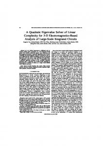
Figure 4. Groundtruth pose (black) and estimated pose of 1st method (red), 2nd method (blue) and geometrical-based method [14] (green).
In Figure 4, we show the accuracy measured in the experiments by plotting eiHe0 in terms of tx, ty, tz, rx, ry, and rz. The figure also shows the results obtained from the ground truth, from the two new methods, and from the geometricbased method. The statistics of the error over the whole testing sequence are shown in Table 1. As it can be observed from the table, the average translational error (tx, ty and tz) for both our methods was less than 10mm. While for the geometric-based method [14] it was over 14mm. Similarly, the maximum error for each of these methods was 27.7mm, 20.6mm, and 52.3mm for the first, second, and the geometric-based methods respectively, and the standard deviations: 0.0057, 0.0036, and 0.0112, respectively. In terms of rotational error, both our methods also proved to be superior to our previous geometric-based method, with the second method showing an even better result than the first one – maximum rotational error in the first method was 1.77 degrees, while in the second method it was only 0.73 degrees.
250
This paper appears in: IEEE International Conference in Robotics and Automation, 2004
From the results, we can conclude that the accuracy in pose estimation of our both methods is quite similar, with the second method being slightly better than the first one. Clearly our new methods outperform the geometric-based method, especially if we consider the maximum errors. Furthermore, we found that the stability of the estimation in both new methods is better than the one in [14]. That fact can be observed in the graphs in Figure 4 in the high frequency noise on top of the curve for the geometric-based method. This noisy estimation in the geometric-based approach can be harmful in our servoing system because it may cause the endeffector to move jerkily.
ACKNOWLEDGMENT
TABLE 1.
Error tx (m.) ty (m.) tz (m.) rx (deg.) ry (deg.) rz (deg.)
Stat. Mean Std Max Mean Std Max Mean Std Max Mean Std Max Mean Std Max Mean Std Max
1st method 0.0059 0.0055 0.0277 0.0097 0.0057 0.0249 0.0039 0.0029 0.0133 0.6721 0.4048 1.5073 0.4395 0.3570 1.7666 0.5273 0.2564 1.0338
On the downside, like any other appearance-based method, our methods cannot be applied when large variations of the object appearance are observed; for example, when the object is observed from a very different angle, or in the presence of occlusions, etc. In these cases, the learnt view of the object may be well hidden for a good match with the model to take place. We are currently developing a strategy that consists of learning different appearance models of the same object when observed from different angles. This multiple AAMs can then be tracked simultaneously while the object is observed from radically different views in the image sequences.
2nd method 0.0098 0.0036 0.0206 0.0041 0.0019 0.0095 0.0042 0.0027 0.0143 0.3857 0.1412 0.5638 0.5507 0.0777 0.7285 0.3246 0.1329 0.6639
Geometric method [14] 0.0147 0.0112 0.0523 0.0079 0.0064 0.0290 0.0042 0.0045 0.0230 0.4819 0.4002 1.6300 0.9510 0.8083 3.7862 0.2286 0.1808 0.9958
The authors would like to thank Ford Motor Company for supporting this project. REFERENCES [1]
[2] [3] [4] [5] [6] [7] [8] [9]
V. CONCLUSION We presented two methods for tracking and pose estimation of generic objects using Active Appearance Models. Feature-based methods, which impose geometric constraints to calculating the pose of the object, tend to be very accurate, and therefore very useful for robotic applications. However, when we compare both our appearance-based methods to a third method based on the geometric features, both methods proved to be a lot better. The error in pose estimation using our second method with 3D parameterization produced a translational error of less than 10mm and a rotational error of little over one half of a degree. Moreover, geometric-based methods require customized algorithms that usually need extensive adaptations when applied for a different object. On the other hand, the creation of appearance models for different objects is a mechanical task that can be easily performed. Another major advantage of appearance-based methods over feature-based methods is in situations where extracting features is not simply done due to cluttered background, complex and irregular features, etc.
[10] [11] [12]
[13] [14]
[15] [16] [17] [18]
R.Hirsh, G.N. DeSouza, and A.C. Kak, “An iterative approach to the handeye and base-world calibration problem,” in Proceedings of 2001 IEEE International Conference on Robotics and Automation, Vol. 1, pp.2171-2176, May 2001. G.N. DeSouza, A Subsumtive, Hierarchical, and Distributed Vision-based Architecture for Smart Robotics, Ph.D. Dissertation., School of Electrical and Computer Engineering, Purdue University, May 2002. A.Kosaka and A.C. Kak, “Stereo vision for Industrial application,” Handbook of Industrial Robotics, edit. S.Y. Nof, pp. 269-294, John Wiley & Son, Inc., NY, 1999. S.K. Nayar, H. Murase, and S.A. Nene, “Learning, Positioning, and Tracking Visual Appearance,” in 1994 IEEE International Conference on Robotics and Automation, Vol. 4, May 1994, pp.3237-3244. J.L. Edwards, “An Active, Appearance-based approach to the Pose Estimation of Complex Objects,” in 1996 IEEE/RSJ International Conference on Intelligent Robots and System , Vol. 3, Nov. 1996, pp. 1458-1465. D.Gennery, “Visual tracking of known three-dimensional objects,” IJCV, 7:243-270, 1992. D.Koller, K.Daniilidis, and H.H. Nagel, “Model-based object tracking in monocular image sequences of road traffic scenes,” IJCV, 10:257-281, 1993. T.F. Cootes, G.J. Edwards, C.J. Taylor, “Active appearance models,” in Proc. European Conference on Computer Vision 1998 (H.Burkhardt & B. Neumann Ed.s). Vol. 2, pp. 484-498, Springer, 1998. T.F. Cootes, C.J. Taylor, Statistical models of appearance for computer vision, in WWW publication, October 2001, Available from http://www.isbe.man.ac.uk/bim/refs.html G.D. Hager, and P.N. Delhumeur, “Efficient Region Tracking with Parameteric Models of Geometry and Illumination,” IEEE Trans. Pattern Analysis and Machine Intelligence, Vol. 20, pp. 1025-1039, Oct. 1998. M. Gleicher, “Projective Registration with Difference Decomposition,” in IEEE Computer Society Conference on Computer Vision and Pattern Recognition, Jun 1997, pp.331-337 M.L. Cascia, S.Sclaroff, and V. Athitsos, “Fast, Reliable Head Tracking under Varying Illumination: An Approach Based on Registration of TextureMapped 3D Models,” IEEE Trans. Pattern Analysis and Machine Intelligence, Vol.22, pp. 322-336, Apr 2000. B.K.P. Horn, “Closed-form solution of absolute orientation using unit quarternions,” Journal of Optical Soc. Am. , Vol. 4, pp. 629-642, 1987. Y.Yoon, G.N. DeSouza, and A.C. Kak, “Real-time Tracking and Pose Estimation for Industrial Objects using Geometric Features,” in 2003 IEEE International Conference on Robotics and Automation, Sep 2003, pp.34733478. O.D. Faugeras, Three-Dimensional Computer Vision, MIT Press, 1993. M. B. Stegmann, B.K. Ersboll, R. Larsen, “FAME--A Flexible Appearance Modeling Environment,” IEEE Trans. Medical Imaging, Vol. 22, No. 10, pp. 1319-1331, Oct 2003. M. B. Stegmann, “Object tracking using active appearance models,” Proc. 10th Danish Conference on Pattern Recognition and Image Analysis, vol. 1, pp. 54-60, DIKU, 2001. J. Ahlberg, “Using the active appearance algorithm for face and facial feature tracking,” in IEEE ICCV workshop on Recognition, Analysis, and Tracking of Faces and Gestures in Real-Time Systems, 2001, pp. 68-72.