Paper No. 01-2264
Using Flow Conservation and Data Redundancy to Estimate Turning Flows at Intersections by
Andrzej P. Tarko Associate Professor of Civil Engineering
[email protected] (765) 494-5027
Robert Lyles Graduate Research Assistant
[email protected]
Purdue University 1284, Civil Engineering Building West Lafayette, IN 47907 Fax: (765) 496-1105
A paper submitted for presentation and subsequent publication at the 80th Annual Transportation Research Board Meeting, Washington D.C., January 2001
Tarko and Lyles
Abstract Traffic volumes at intersections are primary inputs to many transportation studies and analyses. The past works on measuring turning flows at intersections used two distinct approaches. The first one utilized vehicle counts at spots to extract turning volumes. In the second approach, image processing is used to recognize the maneuvers of individual vehicles and count them in proper categories. Neither of the two approaches has yielded a sufficiently reliable method, the primary method of measuring intersection volumes is still based on human observers.
Video detection has the capability of using multiple detectors with flexibility of spot selection. This paper revisits the idea of using spot detection to estimate turning volumes. The flow conservation assumption is used to estimate turning volumes from multiple flow counts and data redundancy is used to improve the estimation accuracy.
The paper presents the formulation of the practical method and its evaluation using both simulated and real data. The proposed method has found to be practical. The quality of video detection counts is important due to a rather small redundancy presented in the problem. The paper gives recommendations helpful in increasing the quality of counts. The proposed method cannot be applied where the number of spots with sufficiently diversified sets of turning flows is too small to obtain a solution. Roundabouts with single-lane approaches are an example.
Key words: vehicle counts, turning volumes, video detection, data collection
1
Tarko and Lyles
Introduction Traffic volumes at intersections are primary inputs to traffic signal warrants, safety and traffic operations analysis, site impact studies, and many other transportation studies. The primary method of measuring intersection volumes is still based on human observers. Although manual counters with built-in memory and PC interfaces help reduce the costs, data collection with people involvement are costly and troublesome.
Several years ago, Indiana Department of Transportation initiated use of video detection for counting flows at intersections. Preliminary benefit-cost estimations indicated that a portable system settable in short time with unattended operation for several hours may bring savings on labor costs that easily exceed the system’s purchase, operations, and maintenance costs. The INDOT Greenfield district was testing a portable system that included a van equipped with three cameras, a 30-foot telescoping pneumatic mast, and the Autoscope system. The counting errors turned out to be considerable. In addition, turning flows could not be measured at intersections where turning movements did not use exclusive approach lanes. The first problem was attributed to the occlusion issue and multiple detection of long vehicles. The second problem was caused by the lack of tracking vehicles when using the Autoscope standard features.
The literature search revealed several past works on measuring turning flows at intersections. They represent two different approaches to the task. The first one extracts turning volumes from several vehicle spot counts. The second one attempts to recognize the maneuvers of individual vehicles and count them in proper categories.
The first approach is represented by methods that have common similarity: they use fewer spot detectors than turning flows. Typically, eight detectors are used at four-leg intersections: four on approaches and four on exits. The primary difference between the methods is the proposed sources of additional information used to complete the data set.
2
Tarko and Lyles Hauer et al. (1981) used the maximum likelihood assumption to estimate turning flows. Van Zuylen (1979) and Mountain and Westwell (1983) proposed to use the turning proportions observed in the past or simply assume some plausible values. Ploss and Keller (1986) used the knowledge of travel times between detectors to progress temporal traffic regularities across the sequence of detectors. They utilized the entropy assumption to deal with the lack of information. Cremer and Keller (1987) applied the method by Ploss and Keller to intersections with entrance and exit detectors. The accuracy of all these methods depends strongly not only on the quality of the spot counts but also on the validity of the assumptions. The second approach requires a method of classifying vehicle maneuvers at the time vehicles are detected. Lu et al. (1988) attempted to identify turning maneuvers by automated recognition of flashing turn signals. This idea involved many serious challenges and was not successful. The latest idea was given by Virkler and Kumar (1998) who used pairs of detectors placed at the corners of intersections to identify turning vehicles. This method is designed only for signalized intersections since it requires the information about signal states to properly classify turns. Other possibilities can be developed from video detection systems that are capable of tracking vehicles across an intersection. Unfortunately, there is no sufficiently reliable tracking system available today. The only commercial system claimed to track vehicles is called VideoTrack. However, it tracks vehicles along user-defined straight paths with the intention to improve spot detection along these paths.
Recent advances in spot detection using vision technology encourage revisiting the first approach that uses spot counts. Today’s systems have a reasonably short setup time and they allow placing large number of detectors at various spots within an image. This paper revisits the idea of using spot detection to estimate turning volumes at intersections. The idea is to use the flow conservation assumption to estimate turning volumes from multiple flow counts and to utilize data redundancy to improve the estimation accuracy.
3
Tarko and Lyles The paper presents the basis of the method and its evaluation using simulated and real data.
Detectors Placement and Flows Assignment The method will be introduced for a four-leg intersection without turning bays (see Fig. 1). Counting turning vehicles at such intersections is difficult since traffic movements (flows) do not use exclusive traffic lanes. Let us initially assume that the camera has been positioned above the intersection or at its corner at a sufficient elevation. Detectors are placed inside the intersection area as defined by the curb lines. Detection spots free of stopped vehicles were selected to increase the counting accuracy.
Figure 1 clearly indicates which flows are counted by which detectors. It should be noted that if a flow is assigned to a detector, ALL vehicles of the flow have to pass the detection spot. This condition allows assigning entire flows to one or more detectors (for example, Flow 2 is assigned to Detectors 1, 3, 4, and 7). The notation for flows and detector counts is introduced in Table 1 and the detector-flow assignment is given in Figure 2.
Another fundamental assumption is that each vehicle passes all the detectors to which the flow containing the vehicle is assigned. This flow conservation assumption is met only approximately if the counting starts at the same time and ends at the same time for all the detectors. Hence, the assumption may be violated at the beginning and end of the counting period. Consequently, the flow preservation assumption is approximately true only if the travel times between the detectors are much shorter than the counting period. That is why, the counting period should be at least several minutes long. In most traffic studies, 15-minute counting intervals or longer are used.
4
Tarko and Lyles
Estimation Method Each detector counts vehicles that belong to assigned flows, which can be described as: Di = ∑ aij F j + ε i ,
(1)
j
where: Di = detector count i, i = 1…16; Fj = turning flow j, j =1…12; aij = detector-flow assignment matrix, aij=1 if detector i counts flow j, = 0 otherwise;
εi = counting error for detector i. The system of Equations 1 carries information sufficient to extract the turning flows. Since there are sixteen detectors and twelve flows, the system of equations can be solved using regression. The error term requires discussion before a proper regression technique can be proposed.
A systematic count error (expected difference from the actual number of vehicles) can be easily accounted for by adding or subtracting from the detector counts the expected bias. After such an adjustment, the remainder error ε has zero mean and non-zero variance and is called random error. Let us discuss the properties of this error. There are two sources of count errors: missed detections and false detections. In the first case, a vehicle is not detected and the corresponding error is -1. In the second case, the detector returns a multiple count when one vehicle passes over the detection zone. The detection error is then the multiple count minus one. Now let us assume that the likelihood of the first error is p, the likelihood of the second error is q, and the average multiple count is n. The expected error associated with one vehicle passage would be (1-p-q)⋅0+p⋅(-1)+q⋅n = q⋅n -
5
Tarko and Lyles p, and since the independent variances sum up, the corresponding total variance is approximately (1-p-q)⋅02+p⋅(-1)2+q⋅n2 = (p + q⋅n2).
There are three assumptions of the detector-count error term. First, we are assuming that the variance of the error is approximately the same for each vehicle. In addition, we are assuming that the errors occur independently one from another. Finally, the third assumption is that counting errors not associated with vehicle passage are negligible (includes vehicles of other flows, pedestrians, other objects, etc.). These assumptions allow expressing the variance of counting error for the stream as the sum of variances generated by D individual vehicles: var ε = D (p+q⋅n2).
(2)
Equation 2 indicates that the standard error grows proportionally to
D . To be able to
use a simple regression, the model in Equation 1 has to be transformed by dividing both its sides by
D . The resulted equation is:
Di = ∑ j
aij Di
Fj +
εi . Di
(3)
Unlike the ε error in Equation 1, the ε / D error in Equation 3 is believed to have uniform variance across detectors. The ordinary least-square regression may now be suitable to find turning flows Fj using Equation 3. Another option, not investigated in this paper, could be the use of a generalized linear regression. The generalized linear regression assumes a parametric relationship between the error variances and the counts as the one in Equation 2. The error-count relationship parameters are estimated together with the turning flows. The last option is to use regression with known covariance matrix for the error term. This approach, although incorporating both error heterogeneity and dependence between errors, requires information about the errors that may be difficult to obtain.
6
Tarko and Lyles
Simulation Tests
Test estimations using simulated data may reveal issues that are not easy to anticipate when developing the method’s concept. We have simulated detector counts for assumed turning flows given in the third column of Table 3 and for detectors' layout shown in Figure 1. The turning flows along with the detector-flow assignment matrix shown in Figure 2 were used to calculate so-called, ideal detector counts that are free of any count errors. Then, the ideal detector counts were contaminated with random errors to simulate actual detector counts that are imperfect. The error for particular detector count D was assumed to be D0.5⋅ε, where ε is the error randomly selected from the range between -3 and 3 (limits assumed arbitrarily). According to the properties of the uniform distribution, the variance of the error was 3⋅D. The error structure is consistent with Equation 2.
Detector counts contaminated with an error were simulated one hundred times. Table 2 provides the ideal detector counts and it summarizes the ranges and standard deviations of the corresponding simulated detector counts. Ordinary regression was used with the model in Equation 3 to estimate the turning flows from each set of simulated detector counts.
The estimated turning flows are presented in Table 3. As expected, the turning flow estimates seem to be unbiased as well as the estimated standard errors. The fourth column in Table 3 gives so-called, reference standard errors of estimation. They have been obtained for the case where each turning flow is measured with its own detector. Similarly to the detector counts, the variance of these errors was 3⋅F. It can be seen that the proposed method is more efficient in estimating the through flows than the direct counting of these flows. The proposed method is marginally better than the direct counting for right turns, and is much worse for left turns. The results reflect the amount
7
Tarko and Lyles of information on the turning flows given by Equations 1 and 3. Each through flow is counted by four detectors. Each right turning flow is counted by three detectors, one of which exclusively counts right turns only. Each left turning flow is counted only by two detectors together with two other flows. It can be concluded that the quality of estimates depends on the number of independent detectors used and the number of flows assigned to these detectors.
The discussion of the error structure given in the previous section involves several rather strong assumptions. Consequently, the actual error variance can be different from the assumed in the model. The effect of such discrepancy has been tested by using three different scaling weights: 1, D0.5, and D. For all three cases, the correct weight was D0.5. Table 4 compares the results obtained for all the three cases. The following expectations were confirmed: (1) Use of incorrect weights does not introduce any bias to the flow estimates. (2) Effectiveness of estimation is comparable in all three cases. (3) The standard errors are considerably underestimated in the two cases of incorrect weights.
Additional simulation tests were performed for T-intersection with eight detectors and six turning flows. Flow estimates were successfully obtained at the expected accuracy. An attempt to apply the method to roundabouts has revealed the issue of co-linearity between rows of the detector-flow matrix. Due to the strong dependence between the circulating flows and the entrance/exit flows, only nine linearly independent counts can be pointed out: four exit counts (detectors), four entrance counts, and one circle count. Any other circle count is the circle count already included plus proper entrance counts minus proper exit counts. The situation is solvable if the approach streams heading to the nearest exit to the right use exclusive traffic lanes as proposed in some modern solutions. In such solutions, four additional independent counts can be obtained from the exclusive lanes. The co-linearity issue occurs even for the considered four-leg intersection after assigning pairs of left turning flows to the inside detectors.
8
Tarko and Lyles
Example Field Application The ability of selecting a sufficient number of spots traversed by certain turning flows has to be checked for a real intersection with a non-ideal position of the camera. In addition, the magnitude and the distribution of counting errors where discussed without referring to any actual data. The presented example is thought to demonstrate the method for real-world conditions where camera’s position is not ideal and other factors such as vehicles occlusion, camera’s motion, etc. are present. The intersection of Yeager Road and Cumberland Avenue in West Lafayette, Indiana, has been selected. It is an all-way stop-controlled intersection with volumes considerably high for this type of intersection. The intersection has two left-turning bays on Cumberland Avenue and single lane approaches on Yeager Road. The intersection with marked twelve turning flows is shown in Figure 3.
Traffic was recorded at the intersection on June 8, 2000, between 2 PM and 3:45 PM. The portable video detection system used for this purpose included a van equipped with 45-foot telescoping mast and two pan/tilt/zoom cameras attached at the top of the mast (Figure 4). There were guide wires running from the top and middle of the mast to stabilize it. The racking system inside the van stored Autoscope, computer interface, and control console for the cameras (Figure 5). The van was positioned on the southwest corner at a 45-degree angle to Cumberland Avenue for the best view. The mast was raised to the maximum height of 45 feet to limit the effect of occlusion. A single camera with an attached wide-angle lens was used. The image in Figure 3 is the actual one seen via the camera. The weather was characterized with clear skies and with mild wind bursts.
To be able to evaluate the accuracy of the method, the ground-truth turning flows were obtained in three consecutive half-an-hour intervals. A Jamar manual recorder was used
9
Tarko and Lyles to obtain the data through playback of the pre-recorded videotape. The ground-truth flows are given in Table 5.
The next step was to use video detection on the image. Figure 6 presents the ‘virtual detector’ layout of 17 detectors of rectangular shape with numbers for identification. We tried to obtain a detector layout such that each detection spot is traversed by all vehicles of certain turning flows. To accomplish this objective, detectors 3, 7, and 13 had to be doubled with a logical AND connection. It means that a vehicle is counted if it activates both the coupled detectors at the same time. Of course, the distance between the detectors in pair has to be shorter than the traversed vehicles’ lengths. The detectorassignment matrix in Figure 7 shows which turning flows have been assigned to which detectors.
The Autoscope 2004 video detection system was used to count vehicles in the same intervals for which the actual flows were obtained. Several detectors were noticed of giving frequent false detections despite our effort to find the best location and size for them. The actual detector counts are shown in Table 6. Their quality has been evaluated with the help of the ideal detector counts. Ideal detector counts given in column three of Table 7 were calculated from equations resulting from the detector-assignment matrix in Figure 7, along with the ground-truth flows in Table 5. The evaluation of the actual counts is presented in Table 7. The detection errors have also been depicted on the scatter plot in Figure 8. Some detectors had tendency to give false detections. After confronting the errors with the detectors’ position, it became obvious that spots experiencing stopped vehicles give false detections more frequent than other spots. Although the absolute errors are not very large, the corresponding relative errors were excessively large (between 97 and 120 %) for three detectors 7, 11, and 13. The three troublesome detectors were temporarily removed from the data and not used in the first estimation of the turning flows.
10
Tarko and Lyles Figure 8 with the three removed detectors shows a tendency in the measurement error to grow with the counts as postulated in the early section. Since this trend is rather weak, ordinary regression was used without scaling the observations. After all, the effect of using incorrect weights is limited to error estimates. The first estimation of turning flows was based on the fourteen detector counts. The results are given in Table 8. The estimation errors are somewhat larger than the detector counting errors. This increase can be attributed to rather small data redundancy (only two detectors in excess of turning flows) and rather large number of flows per detector (six detectors with three flows and four with more than three flows). As expected, less accurate results have been obtained when all the seventeen detectors are used. The effect of incorporating the three incorrect detector counts is shown in Figure 9. Three high-volume turning flows are estimated with a considerably higher error than before. The tendency to increase the estimation error prevails over the reverse tendency in the remainder of flows.
Closure The proposed method turned out to be feasible. It was possible to meet the detector-flow assignment requirements at the example intersection by locating detectors at appropriate spots. It should be kept in mind though, that the camera’s elevation is critical for being able to find such spots due to the occlusion issue, particularly where tall vehicles are present.
The quality of counts is critical for the quality of the turning flow estimates due to rather small data redundancy present in the problem. Motion of the cameras due to wind may cause numerous false counts. This effect can be reduced by placing a detector on a solid background. In addition, the detectors should be located where no stopped vehicles are expected. The combination of a vehicle stopped in a detection spot and a camera motion cause multiple detections of the same vehicle.
11
Tarko and Lyles
It is better to use several cameras if possible and focus on portions of the intersection instead of using one camera with wide-angle lens. Objects far from the camera become small, and undersized detectors have to be placed there at the expense of the counting quality.
The proposed method of extracting turning flows from multiple detector counts is valid and not necessarily associated with video detection. It can be combined with any detection technique that allows fast setting of multiple detectors with localized detection spots. Micro detectors placed on pavement and retrieved after counting can be used instead. Today’s technology allows for building such small devices with their own power source and data storage capabilities.
The limitation of the proposed technique is where the number of spots with sufficiently diversified set of turning flows is too small to extract all the turning flows. Roundabouts with single-lane approaches are an example. On the other hand, roundabouts with exclusive lanes for right-turning flows can be treated with the proposed method.
Acknowledgement The authors thank Mr. Vince Genetti – a participant of the JTRP Summer Internship for assistance in searching literature, and collecting and processing field data.
Literature Cremer, M. and H. Keller (1987). A New Class of Dynamic Methods for the Identification of Origin-destination Flows, Transportation Research, Part B, 21B(2), pp. 117-132. Hauer, E., E. Pagitsas, and B. T. Shin (1981). Estimation of Turning Flows from Automatic Counts, Transportation Research Record 795, Transportation Research Board, Washington, D.C., pp. 1-7.
12
Tarko and Lyles Lu, Y.-J., Y.-H. Hsu, and G. C. Tan (1988). Application of the Image Analysis Technique to Detect Left-Turning Vehicles at Intersections, Transportation Research Record 1194, Transportation Research Board, Washigton, D.C., pp. 120-128. Mountain, L.J. and P. Westwell (1983). The Accuracy of Estimation of Turning Flows from Automatic Counts, Traffic Engineering and Control, No. 1, Vol. 24, pp. 3-7. Ploss, G. and H. Keller (1986). Dynamic Estimation of Origin and Destination Flows from Traffic Counts in Networks, Proceedings of International Conference on Transportation Systems Studies, Tata McGraw-Hill , Delhi, India, pp. 211-221. Van Zuylen, H. J., (1979). The Estimation of Turning Flows on a Junction, Traffic Engineering and Control, No. 20, Vol. 11, pp. 539-541. Vikler, M.R., and N. Kumar (1998). System to identify turning movements at signalized intersections. Journal of Transportation Engineering 124: pp. 607-609.
13
Tarko and Lyles
Table 1 Numbering of the detectors and flows at a four-leg intersection Approach
Movement Right turn Through Left turn
Flow F1 F2 F3
Westbound
Right turn Through Left turn
F4 F5 F6
Southbound
Right turn Through Left turn
F7 F8 F9
Eastbound
Right turn Through Left turn
F10 F11 F12
Northbound
Detector Approach Right turn Inside Exit Approach Right turn Inside Exit Approach Right turn Inside Exit Approach Right turn Inside Exit
Count D1 D2 D3 D4 D5 D6 D7 D8 D9 D10 D11 D12 D13 D14 D15 D16
Table 2 Statistical characteristics of the simulated counts Detector
Ideal Count
D1 D2 D3 D4 D5 D6 D7 D8 D9 D10 D11 D12 D13 D14 D15 D16
1000 300 850 910 900 270 950 890 800 240 850 790 700 210 750 810
Standard Deviation 55 30 50 52 52 28 53 52 49 27 50 49 46 25 47 49
Lowest Count 905 248 763 820 810 221 858 801 715 194 763 706 621 167 668 725
Highest Count 1095 352 937 1000 990 319 1042 979 885 286 937 874 779 253 832 895
14
Tarko and Lyles
Table 3 Results of the simulation test True Ref. Mean Act. Est. Min. Max. Mvnt Flow Turning Std. Est. Std. Std. Value Valu Flows Err. Err. Err. e NL F1 200 24 201 54 54 68 305 NT F2 500 39 498 31 36 426 597 NR F3 300 30 302 28 29 244 357 180 23 179 45 53 83 267 WL F4 WT F5 450 37 445 28 37 386 513 WR F6 270 28 268 27 29 221 321 160 22 165 40 51 54 299 SL F7 ST F8 400 35 400 29 35 336 471 SR F9 240 27 242 24 26 192 294 140 20 143 39 51 65 236 EL F10 ET F11 350 32 347 27 35 286 420 ER F12 210 25 212 26 28 165 267
Table 4 Effect of incorrect weights on the regression results (D0.5 is correct)
Ideal Mvnt Flow Count NL NT NR WL WT WR SL ST SR EL ET ER
F1 F2 F3 F4 F5 F6 F7 F8 F9 F10 F11 F12
200 500 300 180 450 270 160 400 240 140 350 210
Weight = D0.5 Mean Act. Reg. Est. Std. Std. Err. Err. 201 54 54 498 31 36 302 28 29 179 45 53 445 28 37 268 27 29 165 40 51 400 29 35 242 24 26 143 39 51 347 27 35 212 26 28
Weight = 1 Mean Act. Reg. Est. Std. Std. Err. Err. 203 50 25 494 33 7 299 29 10 180 46 26 450 36 8 273 26 10 156 42 27 403 29 7 239 31 13 143 43 8 352 30 22 209 25 11
Weight = D Mean Act. Reg. Est. Std. Std. Err. Err. 195 48 25 501 33 6 302 31 10 186 41 22 447 31 7 270 27 10 152 44 29 398 29 7 243 24 10 145 46 25 350 28 18 208 25 8
15
Tarko and Lyles Table 5 Ground-truth flows Mvnt Flow NL NT NR WL WT WR SL ST SR EL ET ER
F1 F2 F3 F4 F5 F6 F7 F8 F9 F10 F11 F12
Interval (30 min) 1 2 3 44 30 33 42 48 65 32 35 32 18 17 19 54 55 57 12 9 19 10 9 10 34 28 31 8 5 11 12 33 13 46 69 76 19 20 20
Total 107 155 99 54 166 40 29 93 24 58 191 59
Table 6 Actual detector counts Interval (30 min) Detector D1 D2 D3 D4 D5 D6 D7 D8 D9 D10 D11 D12 D13 D14 D15 D16 D17
1 66 129 31 86 23 79 24 67 54 103 30 71 21 108 138 167 126
2 69 165 37 121 22 75 30 98 49 98 60 94 34 133 175 189 138
3 68 152 45 118 19 89 72 105 52 111 29 86 24 128 191 200 158
Actual Total Detector Count 203 446 113 325 64 243 126 270 155 312 119 251 79 369 504 556 422
16
Tarko and Lyles Table 7 Detector counts evaluation
Detector D1 D2 D3 D4 D5 D6 D7 D8 D9 D10 D11 D12 D13 D14 D15 D16 D17
Actual Detector Count 203 446 113 325 64 243 126 270 155 312 119 251 79 369 504 556 422
Ideal Detector Count 191 361 99 294 58 250 59 268 146 322 54 206 40 357 457 594 474
Count (veh)
Error (%)
12 85 14 31 6 -7 67 2 9 -10 65 45 39 12 47 -38 -52
6.3 23.5 14.1 10.5 10.3 -2.8 113.6 0.7 6.2 -3.1 120.4 21.8 97.5 3.4 10.3 -6.4 -11.0
Table 8 Flows estimated from 14 detector counts Interval 1 Flow
Interval 2
Est.
True
F1 F2 F3 F4
42 47 35 19
44 42 32 12
% Error -3.8 11.7 8.9 54.4
Est.
True
50 60 47 18
30 48 35 33
% Error 66.4 25.1 34.8 -46.1
F5 F6 F7 F8
50 27 15 23
46 19 10 34
9.2 43.5 46.6 -32.5
42 32 12 25
69 20 9 28
F9 F10 F11 F12
13 -6 38 29
8 18 54 12
67.6 -131.5 -30.5 141.7
9 8 60 30
5 17 55 9
Interval 3
Total
Est.
True
62 49 42 18
33 65 32 13
% Error 89.0 -24.8 30.5 39.5
Est.
True
155 156 124 54
107 155 99 58
% Error 44.5 0.5 25.1 -6.1
-39.3 58.7 30.6 -9.2
42 47 19 25
76 20 10 31
-45.0 134.5 92.9 -20.2
134 106 46 73
191 59 29 93
-29.9 79.5 57.6 -21.4
80.5 -55.0 8.7 233.3
7 10 59 26
11 19 57 19
-32.8 -50.0 3.7 36.8
30 11 156 85
24 54 166 40
24.3 -78.7 -5.8 112.5
17
Tarko and Lyles
Northbound exit
Northbound inside
Northbound right turn
Northbound approach
Figure 1 Example intersection with detector locations
N_APPR N_RIGHT N_INSIDE N_EXIT W_APPR W_NRIGHT W_INSIDE W_EXIT S_APPR S_RIGHT S_INSIDE S_EXIT E_APPR E_RIGHT E_INSIDE E_EXIT
D1 D2 D3 D4 D5 D6 D7 D8 D9 D10 D11 D12 D13 D14 D15 D16
NL F1 1 0 0 0 0 0 0 1 0 0 0 0 0 0 0 0
NT F2 1 0 1 1 0 0 1 0 0 0 0 0 0 0 0 0
NR F3 1 1 0 0 0 0 0 0 0 0 0 0 0 0 0 1
WL F4 0 0 0 0 1 0 0 0 0 0 0 1 0 0 0 0
WT F5 0 0 0 0 1 0 1 1 0 0 1 0 0 0 0 0
WR F6 0 0 0 1 1 1 0 0 0 0 0 0 0 0 0 0
SL F7 0 0 0 0 0 0 0 0 1 0 0 0 0 0 0 1
ST F8 0 0 0 0 0 0 0 0 1 0 1 1 0 0 1 0
SR F9 0 0 0 0 0 0 0 1 1 1 0 0 0 0 0 0
EL F10 0 0 0 1 0 0 0 0 0 0 0 0 1 0 0 0
ET F11 0 0 1 0 0 0 0 0 0 0 0 0 1 0 1 1
ER F12 0 0 0 0 0 0 0 0 0 0 0 1 1 1 0 0
Figure 2 Detector-flow assignment matrix for the example intersection
18
Tarko and Lyles
WB Approach SB Approach
F6 F5 F7 F4
F8
F3 F2
F9 F1
F10
NB Approach
F11 F12
EB Approach Figure 3 Example intersection of Yeager Road and Cumberland Avenue
Figure 4 The portable video detection system 19
Tarko and Lyles
Figure 5 Racking system inside the portable video detection system
WB Approach SB Approach
D8 D7 D9 D10
D17
D6
D4
D5
D16 D15 D3
D14
D11
D2
D13 D12
D1
NB Approach
EB Approach Figure 6 Autoscope detector layout
20
Tarko and Lyles
Detector D1 D2 D3 D4 D5 D6 D7 D8 D9 D10 D11 D12 D13 D14 D15 D16 D17
NL NT NR WL WT WR SL ST SR EL ET ER F1 F2 F3 F4 F5 F6 F7 F8 F9 F10 F11 F12 0 0 0 1 0 0 0 1 0 0 0 1 1 1 1 0 0 0 0 0 0 0 0 0 0 0 1 0 0 0 0 0 0 0 0 0 0 0 1 0 0 0 1 0 0 0 1 0 0 0 0 1 0 0 0 0 0 0 0 0 0 0 0 0 1 1 0 0 0 0 0 0 0 0 0 0 0 1 0 0 0 0 0 0 0 1 0 0 0 1 0 0 0 1 0 0 0 0 0 0 0 0 1 1 1 0 0 0 1 0 0 0 1 0 0 0 1 0 0 0 0 0 0 0 0 0 0 0 0 1 0 0 0 0 0 0 0 0 0 0 0 0 1 1 0 0 0 0 0 0 0 0 0 0 0 1 1 0 0 1 0 0 0 1 0 0 1 1 1 1 0 0 0 0 1 0 0 0 1 0 1 1 0 1 1 0 1 0 0 1 0 0 1 0 0 0 1 0 1 1 0 1 0 0
Figure 7 Detector flow matrix
21
Tarko and Lyles
Detector Measurement (veh)
700 600 500 400
Counts removed
300 200 100 0 0
100
200
300
400
500
600
700
Ideal Detector Count (veh)
Figure 8 Scatter plot of detector counting accuracy
Estimated Flow (veh/1.5 h)
250
200
Flows estimated from 14 detector counts
150
Flows estimated from 17 detector counts
100
50
0 0
50
100
150
200
250
Actual Flow (veh/1.5h)
Figure 9 The effect of large counting errors 22