An ASAE/CSAE Meeting Presentation
Paper Number: 042162
Comparison of two methods for modeling monthly TP yield from a watershed K. L. White University of Arkansas, 203 Engineering Hall; Fayetteville, AR,
[email protected].
I. Chaubey, PhD University of Arkansas, 203 Engineering Hall; Fayetteville, AR,
[email protected].
B. E. Haggard, PhD USDA-ARS Poultry Production and Product Safety Research Unit, 203 Engineering Hall; Fayetteville, AR,
[email protected].
M. D. Matlock, PhD, PE, CSE University of Arkansas, 203 Engineering Hall; Fayetteville, AR,
[email protected].
Written for presentation at the 2004 ASAE/CSAE Annual International Meeting Sponsored by ASAE/CSAE Fairmont Chateau Laurier, The Westin, Government Centre Ottawa, Ontario, Canada 1 - 4 August 2004
The authors are solely responsible for the content of this technical presentation. The technical presentation does not necessarily reflect the official position of ASAE or CSAE, and its printing and distribution does not constitute an endorsement of views which may be expressed. Technical presentations are not subject to the formal peer review process, therefore, they are not to be presented as refereed publications. Citation of this work should state that it is from an ASAE/CSAE meeting paper. EXAMPLE: Author's Last Name, Initials. 2004. Title of Presentation. ASAE/CSAE Meeting Paper No. 04xxxx. St. Joseph, Mich.: ASAE. For information about securing permission to reprint or reproduce a technical presentation, please contact ASAE at
[email protected] or 269-429-0300 (2950 Niles Road, St. Joseph, MI 49085-9659 USA).
Abstract Watershed models seldom contain detailed components that simulate instream nutrient processes. However, the Soil and Water Assessment Tool (SWAT) watershed model has incorporated some instream modeling capabilities. The goal of this project was to compare total phosphorus (TP) predictions from a watershed model with incorporated instream components to a watershed model linked with a stand alone instream water quality model for War Eagle Creek Watershed in Northwest Arkansas. Our objectives were to: 1) predict monthly TP yields using the SWAT model with instream components active for a watershed (method 1), 2) predict monthly TP yields using a SWAT model without instream components active linked to a QUAL2E model (method 2), and 3) determine if significant differences exist between the two modeling methods. Regression analysis of the two modeling methods provided R2 values of 0.579 and 0.339, respectively. In addition, two variations of the Pearson product-moment correlation (α = 0.05) were evaluated. Statistical results indicated that correlation coefficients and regression slopes for the two data sets were not significantly different. This implies that no additional knowledge was gained concerning monthly TP yields from the watershed by adding the detailed instream, QUAL2E model to the SWAT model. Therefore, the SWAT model with active instream components (method 1) sufficiently predicts TP yields from War Eagle Creek Watershed. Although War Eagle Creek Watershed is not greatly urbanized (only 0.5% by area), point and nonpoint P sources are present and included in the modeling process. Hence, monthly TP yields from watersheds with similar characteristics can be estimated using the SWAT model (method 1). Keywords. SWAT model, QUAL2E model, phosphorus, watershed
The authors are solely responsible for the content of this technical presentation. The technical presentation does not necessarily reflect the official position of ASAE or CSAE, and its printing and distribution does not constitute an endorsement of views which may be expressed. Technical presentations are not subject to the formal peer review process, therefore, they are not to be presented as refereed publications. Citation of this work should state that it is from an ASAE/CSAE meeting paper. EXAMPLE: Author's Last Name, Initials. 2004. Title of Presentation. ASAE/CSAE Meeting Paper No. 04xxxx. St. Joseph, Mich.: ASAE. For information about securing permission to reprint or reproduce a technical presentation, please contact ASAE at
[email protected] or 269-429-0300 (2950 Niles Road, St. Joseph, MI 49085-9659 USA).
Introduction Excessive nutrient yields was identified in a 2000 U.S. Environmental Protection Agency (USEPA) report as the leading cause of impairment in assessed lakes and reservoirs. The dominant sources of these nutrients were suggested to be a result of upstream watershed activities such as agriculture, hydrological modifications, and urban runoff (USEPA, 2000). The occurrence of increased nutrient loads into reservoirs is of particular concern because they accelerate eutrophication. Eutrophic conditions decrease the longevity of reservoirs in their ability to meet designated uses. For example, a drinking water reservoir that continues to receive excessive nutrient loads may experience premature decreases in oxygen concentrations, increases in suspended solids, progression from a diatom population to a bluegreen or green algae population, changes in food web structure and fish species composition, and decreasing light penetration (OECD, 1982; Henderson-Sellers and Markland, 1987). These characteristics can result in undesirable effects such as release of reduced gases (methane, hydrogen sulfide, and ammonia) that degrade the taste of drinking water and are potentially toxic (Henderson-Sellers and Markland, 1987). Management of reservoir nutrient loading requires an understanding nutrient transport and delivery from the watershed-stream system. Nutrients are generally transported from the landscape during runoff events and are carried into the stream system. In the stream, they undergo biotic and abiotic cycling. Nutrients may also enter stream flow from other sources such as groundwater recharge and point source effluent discharges. Nutrients are eventually delivered by stream flow to downstream reservoirs. Nutrient transport and delivery from a watershed-stream system is most efficiently evaluated using computer models. Computer models are available that simulate nutrient transport in a watershed and instream nutrient processes; however, they are normally not incorporated into one model. Generally, landscape models predict flow volume, nutrient yields, and sediment yield leaving the landscape from a specifically defined boundary to a certain outlet point. Landscape or watershed models seldom contain detailed instream algorithms that simulate instream nutrient cycling. However, the Soil and Water Assessment Tool (SWAT) model has incorporated some ability to simulate instream nutrient processes. SWAT developers modified equations from the instream water quality model, QUAL2E, and provided options within the SWAT model to include or exclude these calculations in watershed model simulations (Neitsch, et al., 2001). However, there is uncertainty regarding the ability of the SWAT model to substitute for a complete instream water quality model in predicting nutrient yields from a watershed (Houser and Hauck, 2002). While there are limitations in the ability of watershed models to simulate instream processes, there are also limitations with currently available, stand alone, instream water quality models. Instream water quality models do not estimate yields from their respective drainage areas. Therefore, these flow volumes and constituent yields must be determine by another method and input into the water quality model (e.g., CE-QUAL-RIV-1) (USACE, 1995). Another limitation is that many instream water quality models do not possess spatial distinctions such as stream reaches and tributaries and are classified as point models (e.g., AQUATOX) (Park and Clough, 2004). Instream water quality models also are commonly steady state and provide little to no dynamic simulation abilities (e.g., QUAL2E) (Brown and Barnwell, 1987). The goal of this project was to compare total phosphorus (TP) predictions from a watershed model with incorporated instream components to a watershed model linked with a stand alone instream water quality model to determine if significant differences occurred in their predictive abilities. Our objectives were to: 1) predict monthly TP yields from the SWAT model
2
with instream components active for a watershed (method 1), 2) predict monthly TP yields from a SWAT model without instream components active that is loosely linked to a QUAL2E model (method 2), and 3) determine if significant differences exist between values predicted with both modeling methods and measured values.
Study Site The study site used in this investigation is the War Eagle Creek Watershed in Northwest Arkansas. War Eagle Creek is one of the main tributaries to Beaver Reservoir, which is the primary drinking water supply for Northwest Arkansas. War Eagle Creek Watershed encompasses approximately 68,100 ha with land use distributions of 63.7% forest, 35.6% pasture, 0.5% urban, and 0.2% water (CAST, 2002). The watershed was delineated into 13 subbasins using the delineation tool in the SWAT model ArcView interface (Fig. 1).
Figure 1. War Eagle Creek Watershed with 13 delineated subasins and streams in Northwest Arkansas
3
Methods SWAT Model The SWAT model is a widely used, physically based and GIS-linked, watershed model developed by US Department of Agriculture – Agriculture Research Service (USDA-ARS). It functions on a continuous time step with input options for hydrology, nutrients, erosion, land management, main channel processes, water bodies, and climate data. The SWAT model predicts the influence of land management practices on constituent yields from a watershed. The model includes agricultural components such as fertilizer, crops, tillage options, and grazing and has the capability to include point source yields (Neitsch et al., 2001). We used the ArcView interface with SWAT2000 (AVSWAT) in this application, which was the current version of the model at the beginning of the project. Mandatory GIS input files needed for the SWAT model included the Digital Elevation Map (DEM), land cover, and soil layers. The following GIS data were used to develop the War Eagle Creek Watershed model to simulate watershed response from 2001 to 2002: 30-meter DEM (US Geological Survey), rf3 stream shape file (EPA BASINS), 28.5-m 1999 land use and land cover image file (CAST, 2002), and STATSGO soils shape file (EPA BASINS). Based on threshold specifications and the DEM, AVSWAT was used to delineate the watershed into 13 subbasins. Point and nonpoint sources were included in the model such as, waste water treatment plant (WWTP) effluent discharge, animal production, and commercial fertilizer usage. Weather data from stations within the region were incorporated to provide the most representative precipitation and temperature data available. Hydrologic/water quality response of War Eagle Creek Watershed was simulated using the SWAT model with active instream components. The War Eagle Creek SWAT model was calibrated using data collected at the US Geological Survey (USGS) gauging station: War Eagle Creek near Hindsville (USGS 07049000) (Fig. 1). About twice-a-month water quality sampling occurred at the USGS gauge, therefore daily measured water quality concentrations were not available. Daily concentrations were estimated from collected samples using LOADEST2 software (Crawford, 1991; 1996). The SWAT model was calibrated and validated for flow volume, sediment yield, TP yield, and NO3-N plus NO2-N yield at annual and monthly time scales. To calibrate and validate the War Eagle Creek SWAT model for flow, data was available from 1999 to 2002. Flow calibration was conducted on data from 1999 to 2000, while flow validation was performed using 2001 and 2002 flow data. However, only 2001 and 2002 data was available for sediment and nutrients. Sediment and nutrients were calibrated using 2001 data and validated using 2002 data. Three statistical objective functions were used in the calibration of the War Eagle Creek SWAT model. We defined the multi-objective function as the optimization of the following three statistics for each of the previously identified variables. SWAT model annual calibration was performed by minimizing the RE (%) at the gauge location:
RE (%) =
(O − P ) *100 O
(1)
where O is the measured value and P is the predicted output.
4
The SWAT model was further calibrated monthly using the Nash-Sutcliffe Coefficient (RNS2), which is defined as: n
2
R NS = 1 −
∑ (O
i =1 n
∑ (O i =1
i
− Pi )
2
(2)
− O avg )
2
i
where O is measured values, P is predicted outputs and i = number of values (Nash and Sutcliffe, 1970). Monthly coefficient of determination (R2) was also calculated since RNS2 is sensitive to outliers (Kirsch et al., 2002). The R2 statistic is calculated as: n (Oi − Oavg )(Pi − Pavg ) ∑ 2 i =1 R = 0 .5 n n (O − O )2 (P − P )2 ∑ avg i avg ∑ i i =1 i =1
2
(3)
QUAL2E Model The QUAL2E model is a 1-dimensional instream water quality model that simulates interactions between constituents such as nutrients, algae production, benthic oxygen demand, carbonaceous oxygen uptake, and atmospheric aeration (Brown and Barnwell, 1987). The QUAL2E model was chosen to simulate instream water quality response because of its ability to simulate a stream system comprised of tributaries and headwater reaches. It was also selected because it has been widely implemented since its completion in 1985 to simulate water quality response to changes in pollutant yields (Thakar and Rogers, 1994; Ning et al., 2001). The steady state characteristic of the QUAL2E model limits its appropriateness to predict constituent dynamics in a continuously changing system (Zhang et al., 1996). For example, the QUAL2E model requires flow rate and constituent yields to remain constant. To accommodate for this limitation, War Eagle Creek was modeled for three different seasons during the year: summer (or low flow), fall (low flow after leaf abscission), and winter-spring (high flow). Summer, fall, and winter-spring were considered by months as Jul. through Sept., Oct. through Dec., and Jan. through Jun., respectively. These seasons were chosen to account for differences in stream flow and nutrient dynamics that occur throughout the year (Haggard et al., 2003). QUAL2E model inputs that describe the stream’s physical characteristics (length, slope, network) did not change between the three QUAL2E models. The War Eagle Creek Watershed was divided into thirteen reaches in the QUAL2E model. Each subbasin (as defined in Fig. 1) was identified as a separate reach. Reach hydraulic characteristics, such as slope and cross section features were measured in the field using GPS surveying equipment. In some stream reaches, riparian cover prevented GPS surveying. For these reaches, GIS data and ESRI software were employed to acquire stream slopes. Initial conditions for chlorophyll-a, organic-N, NH3-N, NO2-N, NO3-N, organic-P, and dissolved P were estimated for each QUAL2E model reach by season using SWAT model monthly predicted outputs. The SWAT model outputs used as input for the QUAL2E model were from simulations of the calibrated SWAT model with the instream components turned ‘off’
5
or inactive. For each constituent, QUAL2E model reach, and season; SWAT model predicted yields were calculated. These yields were divided by the respective total flow to obtain a flowweighted concentration for each season. These concentrations became the values for QUAL2E model initial conditions. Similarly to the QUAL2E model inputs that described initial conditions, QUAL2E model headwater source inputs were derived for each season and reach from SWAT predicted values. Headwater source inputs refer to flow and constituent concentrations that enter the river system as a tributary or headwater stream. Initial condition and headwater stream values for temperature and DO were estimated using field data collected for each reach during the three seasons. These physicochemical parameters were collected during the summer and fall of 2003 and winter-spring of 2004. Field measured values were used instead of SWAT prediction for temperature and DO because of SWAT process deficiencies for simulating DO, lack of calibration data for temperature and DO, and temperature not being a readily available SWAT model output. To simulate groundwater, transmission losses, and evaporation occurring in the main reach; QUAL2E model incremental flows were defined. SWAT model output for groundwater, transmission losses, and evaporation was summed into one flow value to be input into the QUAL2E model as incremental flows. Constituent concentrations (chlorophyll-a, organic-N, NH3-N, NO2-N, NO3-N, organic-P, and dissolved P) may also be included in the QUAL2E model incremental inputs; however, we assumed that these values were approximately zero. This assumption was based on the insensitivity of QUAL2E predicted outputs to changes in incremental constituent concentration inputs. Climatology is represented in the QUAL2E model by air temperature, dew point temperature, wind direction, wind speed, and cloudiness. Measured data from the Huntsville weather station located in the watershed were used in this study. The three seasonal QUAL2E models were calibrated for the years 2001-2002 using relative error as described in Eq. (1).
Comparison of Two Modeling Methods Monthly TP yields were compared using results obtained from the SWAT model (method 1) and the SWAT model linked to a stand alone QUAL2E model (method 2) to determine if predicted monthly TP yields were significantly different from each other. Two variations of the Pearson product-moment correlation coefficient (α = 0.05) were used to assess the two modeling methods by tested: (1) the null hypothesis that the correlation between the two variables in the underlying populations represented by the two samples were equal (Eq. 4), and (2) the null hypothesis that the slopes of two regression lines obtained from two independent samples were equal (Eq. 5) (Sheskin, 2000). The first Pearson product-moment correlation was evaluated such that:
H o : ρ1 = ρ 2 H a : ρ1 ≠ ρ 2
(4)
where ρ = the population correlation, 1 refers values from the SWAT model (method 1) and 2 refers to values from the SWAT model linked to a QUAL2E model (method 2). The second statistic evaluated the same data set with the following hypotheses:
H o : β 11 = β12 H a : β 11 ≠ β 12
(5)
6
where β1 = slope of a regression line.
Results and Discussion Average monthly statistical results for the War Eagle Creek SWAT model (method 1) are provided in Table 1. These values were calculated by averaging the SWAT model monthly predictions for 2001 and 2002. Similarly, measured monthly TP yields for War Eagle Creek Watershed were tabulated from measured water quality and stream discharges. Monthly TP yields from the SWAT model linked to the QUAL2E model (method 2) are also presented. Since the QUAL2E model is a steady state model and three seasonal QUAL2E models were built to sufficiently represent the differences in P dynamics throughout the year, months of the same season are characterized by the same TP yield. Table 1. Measured TP yields (USGS gauge) and model predicted TP yields (SWAT model and SWAT model linked with the QUAL2E model)
Month January February March April May June July August September October November December
USGS gauge (kg TP) 959 2,622 2,143 2,591 629 635 195 157 85 193 110 2,488
SWAT (method 1) (kg TP) 1,710 1,295 1,241 1,917 593 855 735 864 777 585 322 1,297
SWAT plus QUAL2E (method 2) (kg TP) 988 988 988 988 988 988 281 281 281 719 719 719
Regression was performed comparing both modeling methods predicted monthly TP yields to measured TP yields. Regression coefficients and correlations are presented in Table 2. The R2 regression statistic represents the square of the sample correlation coefficient, r. Table 2. Regression statistics from comparing measured and predicted TP monthly values using modeling methods 1 and 2 Modeling method
Regression statistics R
β11
β02
SWAT model (method 1)
0.58
0.34
650
SWAT model linked to QUAL2E model (method 2)
0.34
0.17
570
2
1
Slope of the regression line
2
Y-intercept of the regression line
7
The resulting z (Fisher’s z) value from testing the null hypothesis in Eq. 4 was 0.703, which was less than z0.05 (1.96), hence we failed to reject the null hypothesis. This test indicated that the populations represented by the two samples had correlation values that were equal. In addition, the test statistic for the null hypotheses in Eq. 5 was t (Student’s t distribution) = 1.51. The t0.05 value is 2.09, which is less than 2.09, and therefore we failed to reject the null hypothesis. This indicated that the slopes of the regression lines of the two data sets were not significantly different. The results from this study suggested that the two modeling methods simulated monthly TP yields that were not significantly different. This implies that no additional knowledge was gained concerning monthly TP yields from the watershed by adding the detailed instream, QUAL2E model to the SWAT model. TP sources that are characterized by different transport and delivery mechanisms were incorporated into the SWAT model (e.g., WWTP effluent, cattle manure, commercial fertilizer, poultry litter). Land cover composition, which also influences TP transport and delivery within a watershed, was detailed within the model. Results from this project suggest that watershed with similar P sources and land cover would also be sufficiently represented by a SWAT model with active instream components. Watersheds with substantially different sources of P and/or land cover might not have the same result.
Conclusion Objective 1: The SWAT model was successfully used to simulate the War Eagle Creek Watershed to estimate monthly TP yields for 2001 and 2002. Objective 2: The SWAT model was successfully linked to an independent QUAL2E model to predict monthly TP yields for 2001 and 2002. Objective 3: No statistically significant differences were observed between the predicted monthly TP yields of the two modeling approaches (the SWAT model (method 1) and the SWAT model linked to a QUAL2E model (method 2)) when compared to measured data. The results of this study indicated that there were no added benefits to linking an instream model (QUAL2E model) to a SWAT model to predict monthly yields compared to using the SWAT model with active instream components. The two modeling methods predicted statistically similar monthly TP yields at the War Eagle Creek Watershed. However, the steady state limitation of the QUAL2E model hinders its ability to simulate dynamic P processes, such as nonpoint sources of P and P resuspension within the stream channel. This suggests that if an instream model were available that possessed greater spatial and temporal resolutions than the QUAL2E model, there would be a need to reevaluate this concept by linking the SWAT model with the improved instream water quality model.
Acknowledgements We would like to acknowledge the Division of Agriculture at the University of Arkansas and the Arkansas Soil and Water Conservation Commission for their financial support. In addition, we would like to thank the ecological engineering undergraduate field workers, Chad Cooper, and Eylem Mutlu for their assistance in completing the field work.
8
References Brown, L. C. and T. O. Barnwell, Jr., 1987. The enhanced stream water quality models QUAL2E and QUAL2E-UNCAS: Documentation and User Manual. Tufts University and US EPA, Athens, Georgia. CAST, 2002. 1999 Land use/ land cover data. Available at: http://www.cast.uark.edu/cast/geostor/. Accessed in January 2004. Coombs, T. R., and F. C. Watson, 1997. Computational Fluid Dynamics. 3rd ed. Wageningen, The Netherlands: Elsevier Science. Crawford, C. G., 1991. Estimation of Suspended-Sediment Rating Curves and Mean SuspendedSediment Yields. Journal of Hydrology 129: 331-348. 1996. Estimating Mean Constituent Yields in Rivers by the Rating-Curve and FlowDuration, Rating-Curve Methods. PhD dissertation, Bloomington, Indiana: University of Bloomington. Haggard, B. E., P. A. Moore Jr, I. Chaubey, and E. H. Stanley, 2003. Nitrogen and phosphorus concentrations and export from an Ozark Plateau catchment in the United States. Biosystems Engineering 86(1):75-85. Houser, J.B. and L.M. Hauck, 2002. Analysis of the in-stream water quality component of SWAT (Soil and Water Assessment Tool). Proceedings of the TMDL Environmental Regulations Conference. ASAE. St. Joseph, MI. 52-55 Henderson-Sellers, B. and H. R. Markland, 1987. Decaying Lakes: The origins and control of cultural eutrophication. Great Britain: John Wiley & Sons Ltd. Kirsch, K.J., A. Kirsch, and J.G. Arnold, 2002. Predicting Sediment and Phosphorus Loads in the Rock River Basin using SWAT. Transactions of the American Society of Agricultural Engineers 45(6):1757-1769. Nash, J. E. and J. V. Sutcliffee, 1970. River Flow Forecasting Through Conceptual Models: Part I. A Discussion of Principles. Journal of Hydrology 10(3):282-290. Neitsch, S.L., J. G. Arnold, J. R. Kiniry, and J. R. Williams, 2001. Soil and Water Assessment Tool Theoretical Documentation Version 2000. http://www.brc.tamus.edu/swat/manual. Ning, S.K., N.B. Chang, L. Yang, H.W. Chen, and H.Y. Hsu, 2001. Assessing pollution prevention program by QUAL2E simulation analysis for the Kao-Ping River Basin, Taiwan. Journal of Environmental Management 61:61-76. OECD, 1982. Eutrophication of waters: monitoring, assessment, and control, organization of economic cooperation and development. Paris, p 154. Park, R. A. and J. S. Clough, 2004. AQUATOX (release 2): Modeling environmental fate and ecological effects in aquatic ecosystems. Vol 2: Technical documentation. USEPA, Washington DC. Sheskin, D. J., 2000. Handbook of Parametric and Nonparametric Statistical Procedures Second edition. Boca Raton, FL.: CRC Press. Thakar, G.R. and J. Rogers, 1994. Use of EPA’s Qual-2E model to predict water quality in an Arkansas River system. New Waves: March 1994. 7(1) USEPA, 2000. National Water Quality Inventory Report. www.epa.gov/305b/2000report USACE, 1995. CE-QUAL-RIV1: A dynamic, one-dimensional (longitudinal) water quality model for streams. Instruction Report EL-95-2. Vicksburg, MS. Zhang, J., T. S. Tisdale, and R. A. Wagner, 1996. A basin scale phosphorus transport model for south Florida. Applied Engineering in Agriculture. 12(3):321-327.
9