Case Studies in Bayesian Computation using INLA - CiteSeerX

Case Studies in Bayesian Computation using INLA Sara Martino and H˚avard Rue

Abstract Latent Gaussian models are a common construct in statistical applications where a latent Gaussian field, indirectly observed through data, is used to model, for instance, time and space dependence or the smooth effect of covariates. Many well known statistical models, such as smoothing-spline models, space time models, semi-parametric regression, spatial and spatio-temporal models, log-Gaussian Cox models, and geostatistical models are latent Gaussian models. Integrated Nested Laplace approximation (INLA) is a new approach to implement Bayesian inference for such models. It provides approximations to the posterior marginals of the latent variables which are both very accurate and extremely fast to compute. Moreover, INLA treats latent Gaussian models in a general way, thus allowing for a great deal of automation in the inferential procedure. The inla program, bundled in the R library INLA, is a prototype of such black-box for inference on latent Gaussian models which is both flexible and user-friendly. It is meant to, hopefully, make latent Gaussian models applicable, useful and appealing for a larger class of users.

1 Introduction Latent Gaussian models are an apparently simple but very flexible construct in statistical applications which covers a wide range of common statistical models spanning from (generalized) linear models, (generalized) additive models, smoothing spline models, state space models, semi-parametric regression, spatial and spatiotemporal models, log-Gaussian Cox processes and geostatistical and geoadditive models. Sara Martino Department of Mathematical Sciences, Norwegian University for Science and Technology, N-7491 Trondheim, Norway, e-mail: [email protected] H˚avard Rue Department of Mathematical Sciences, Norwegian University for Science and Technology, N-7491 Trondheim, Norway, e-mail: [email protected]

1

2

Sara Martino and H˚avard Rue

In these models, the latent Gaussian field serves as a flexible and powerful tool to model non-linear effects of covariates, group specific heterogeneity, as well as space and time dependencies among data. Bayesian inference on latent Gaussian models is not straight forward since, in general, the posterior distribution is not analytically available. Markov Chain Monte Carlo (MCMC) techniques are, today, the standard answer to this problem and several ad hoc algorithms have been developed in recent years. Although in theory always possible to implement, MCMC algorithms applied to latent Gaussian models come with a wide range of problems in terms of convergence and computational time. Moreover, the implementation itself might often be problematic, especially for end users who might not be experts in programming. Integrated Nested Laplace approximation (INLA) is a new tool for Bayesian inference on latent Gaussian models when the focus is on posterior marginal distributions [20]. INLA substitutes MCMC simulations with accurate, deterministic approximations to posterior marginal distributions. The quality of such approximations is extremely high, such that even very long MCMC runs could not detect any error in them. A detailed description of the INLA method and a thorough comparison with MCMC results can be found in [20]. INLA presents two main advantages over MCMC techniques. The first and most outstanding is computational. Using INLA results are obtained in seconds and minutes even for models with a huge dimensional latent field, where a well build MCMC algorithm would take hours or even days. This is also due to the fact that INLA is naturally parallelized, thus making it possible to exploit the new trend of having multi-core processors. The second, and not less important advantage, is that INLA treats latent Gaussian models in a unified way, thus allowing greater automation of the inference process. The core of the computational machinery, automatically adapts to any kind of latent field so that, from the computational point of view, it does not matter if we deal with, for example, spatial or temporal models. In practice INLA can be used almost as a black box to analyze latent Gaussian models. A prototype of such program, inla, together with a user-friendly R interface (INLA library) is already available from the web-site www.r-inla.org. Its goal is to make the INLA approach available for a larger class of users. The hope is that near instant inference and simplicity of use will make latent Gaussian models more applicable, useful and appealing for the end user. The purpose of this paper is to give an overview of models to which INLA is applicable. We will present a series of case studies ranging from generalized linear models to spatially varying regression models to survival models, solved using the INLA methodology through the INLA library. The structure of this article is as follows. Section 2 describes latent Gaussian models and their main features. Section 3 and Section 4 briefly introduce the INLA approach and the INLA library. In Section 5 three case studies are analyzed. They include a GLMM model with overdispersion, different models for spatial analysis and a model for survival data. We end with a brief discussion in Section 6.

Case Studies in Bayesian Computation using INLA

3

2 Latent Gaussian Models Latent Gaussian models are hierarchical models which assume a n-dimensional Gaussian field x = {xi : i ∈ V } to be point-wise observed through nd conditional independent data y. Both the covariance matrix of the Gaussian field x and the likelihood model for yi |x can be controlled by some unknown hyperparameters θ . In addition, some linear constraints of the form Ax = e, where the matrix A has rank k, may be imposted. The posterior then reads:

π (x, θ | y) ∝ π (θ ) π (x | θ )

∏ π (yi | xi , θ ).

(1)

i∈I

As the likelihood often is not Gaussian, this posterior density is not analytically tractable. A slightly different point of view to look at latent Gaussian models is to consider structured additive regression models; these are a flexible and extensively used class of models, see for example [8] for a detailed account. Here, the observation (or response) variable yi is assumed to belong to an exponential family where the mean µi is linked to a structured additive predictor ηi through a link-function g(·), so that g(µi ) = ηi . The likelihood model can be controlled by some extra hyperparameters θ1 . The structured additive predictor ηi accounts for effects of various covariates in an additive way: nf

ηi = β0 + ∑ w ji f j=1

( j)

nβ

(u ji ) + ∑ βk zki + εi .

(2)

k=1

Here, the {βk }’s represent the linear effect of covariates z. The { f ( j) (·)}’s are unknown functions of the covariates u. These can take very many different forms: nonlinear effects of continuous covariates, time trends, seasonal effects, i.i.d.random intercepts and slopes, group specific random effects and spatial random effects can all be represented through the { f ( j) }’s functions. The wi j are known weights defined for each observed data point. Finally, εi ’s are unstructured random effects. A latent Gaussian model is obtained by assigning x = {{ f ( j) (·)}, {βk }, {ηi }} a Gaussian prior with precision matrix Q(θ2 ), with hyperparameters θ2 . Note that we have parametrized the latent Gaussian field so that it includes the ηi ’s instead of the εi ’s, in this way some of the elements of x, namely the ηi ’s, are observed through the data y. This is mainly due to the fact that the INLA library requires each data point yi to be dependent on the latent Gaussian field only through one single element of x, namely ηi . For this reason, a small random noise, εi , with high precision is always automatically added to the model. The definition of the latent model is completed by assigning the hyperparameters θ = (θ1 , θ2 ) a prior distribution. In this paper the latent Gaussian models are assumed to satisfy two basic properties: First, the latent Gaussian model x, often of large dimension, admits conditional independence properties. In other words it is a latent Gaussian Markov random field (GMRF) with a sparse precision matrix Q, [18]. The second property is that the di-

4

Sara Martino and H˚avard Rue

mension m of the hyperparameter vector θ is small, say ≤ 6. These properties are satisfied by many latent Gaussian models in the literature. Exceptions exist, geostatistical models being the main one. INLA can still be applied to geostatistical model using different computational machinery or using a Markov representation of the Gaussian field (see [7] and the discussion contribution from Finn Lindgren in [20])

3 Integrated Nested Laplace Approximation Integrated Nested Laplace approximation (INLA) is a new approach to statistical inference for latent Gaussian models introduced by [19] and [20]. In short, the INLA approach provides a recipe for fast Bayesian inference using accurate approximations to the marginal posterior density for the hyperparameters π˜ (θ |y) and for the full conditional posterior marginal densities for the latent variables π˜ (xi |θ , y), i = 1, . . . , n. The approximation for π (θ |y) is based on the Laplace approximation [22], while for π (xi |θ , y) three different approaches are possible: A Gaussian, a full Laplace and a simplified Laplace approximation. Each of these has different features, computing times and accuracy. The Gaussian approximation is the fastest to compute but there can be errors in the location of the posterior mean and/or errors due to the lack of skewness [19]. The Laplace approximation is the most accurate but its computation can be time consuming. Hence in [20] the simplified Laplace approximation is introduced. This is fast to compute and usually accurate enough. Posterior marginals for the latent variables π˜ (xi |y) are then computed via numerical integration as:

π˜ (xi |y) =

Z

π˜ (xi |θ , y)π˜ (θ |y) d θ

K

≈

∑ π˜ (xi |θk , y)π˜ (θk |y) ∆k

(3)

k=1

Posterior marginals for the hyperparameters π˜ (θ j |y), J = 1, . . . , m are computed in a similar way. The choice of the integration points θk can be done using two strategies: The first, more accurate but also time consuming, is a to define a grid of points covering the area where most of the mass of πe(θ |y) is located (GRID strategy). The second strategy, named central composit design (CCD strategy), comes from the design problem literature and consists in laying out a small amount of ’points’ in a m-dimensional space in order to estimate the curvature of πe(θ |y), see [20] for more details on both strategies. In [20] it is suggested to use the CCD strategy as a default choice. Such strategy is usually accurate enough for the computation of π˜ (xi |y), while a GRID strategy might be necessary if one is interest in a accurate estimate of π˜ (θ j |y). The approximate posterior marginals obtained from such procedure can then be used to compute summary statistics of interest, such as posterior means, variances or quantiles.

Case Studies in Bayesian Computation using INLA

5

INLA can also compute, as by-product of the main computations, other quantities of interest like Deviance Information Criteria (DIC) [21], marginal likelihoods and predictive measures as logarithmic score [11] and the PIT histogram [6], useful to detect outliers and to compare and validate models. Different strategies to assess the accuracy of the various approximations for the densities xi |θ , y are described in [20]. The INLA approximations assumes the posterior distribution π (x|θ , y) to be unimodal and fairly regular. This is usually the case for most real problem and data sets. INLA can, however, deal to some extent with the multimodality of π (θ |y), provided that the modes are sufficiently closed. See the discussion contributions of Ferreira and Hodges and the author’s reply in [20]. Theory and practicalities about INLA are deeply analyzed in [20] and will not be repeated here. Loosely speaking we can say that INLA fully exploits all main features of the latent Gaussian models described in Section 2. Firstly, all computations are based on sparse matrix algorithms which are much faster than the corresponding algorithms for dense matrix. Secondly, the presence of the latent Gaussian field and the usual “well-behavior” of the likelihood function justify the accuracy of the Laplace approximation. Finally, the small number of hyperparameters θ makes the numerical integration in equation (3) computationally feasible.

4 The INLA package for R Computational speed is one of the most important components of the INLA approach, therefore special care has to be put in the implementation of the required algorithms. All computations required by the INLA methodology are efficiently performed by the inla program, written in C based on the GMRFLib-library which includes efficient algorithms for sparse matrices [18]. Both the inla program and the GMRFLib-library, in addition, use the OpenMP (see http://www.openmp.org) to speed up the computations for shared memory machines, i.e. multicore processors, which are today standard for new computers. Moreover, the inla program is bundled within a R library called INLA in order to ease its usage. The software is open-source and can be downloaded from the web site www.r-inla.org. It is running under Linux, MAC and Windows. On the same web site documentation and a large sample of applications are also provided.

5 Case studies The following examples are meant to give an overview of the range of application of the INLA methodology. All examples are implemented using the INLA library on a dual-core 2.5GHz laptop. The R code is reported where it was considered helpful, the rest of the R code can be downloaded from the www.r-inla.org web site in the Download section.

6

Sara Martino and H˚avard Rue

5.1 A GLMM with over-dispersion The first example is a generalized linear mixed model with binomial likelihood, where random effects are used to model within group extra variation. The data concern the proportion of seeds that germinated on each of m = 21 plates arranged in a 2 × 2 factorial design with respect to seed variety and type of root extract. The data set was presented by [5] and analyzed among other by [3], this example is also included in the WinBUGS/OpenBUGS manual [15]. In [9] the authors perform a comparison between the INLA and the maximum likelihood approach for this particular data set. The sampling model is yi |ηi ∼ Binomial(ni , pi ) where, for plate i = 1, . . . , m, yi is the number of germinating seeds (variable name (vn): r) and ni the total number of seeds ranging from 4 to 81 (vn: n), and pi = logit−1 (ηi ) is the unknown probability of germinating. To account for between plate variability, [3] introduce plate-specific random effects, and then fit a model with main and interaction effects:

ηi = β0 + β1 z1i + β2 z2i + β3 z1i z2i + f (ui )

(4)

with z1i and z2i representing the seed variety (vn: x1) and type of root extract (vn: x2) of plate i. We assign βk , k = 0, . . . , 3 vague Gaussian priors with known precision. Moreover, we assume f (ui )|τu ∼ N (0, τu−1 ), i = 1, . . . , 21, so that the general f () function in Equation (2) here takes the simple form of i.i.d. random intercepts. To complete the model we assign the hyperparameter a vague Gamma prior τi ∼ Gamma(a, b) with a = 1 and b = 0.001. As explained in Section 2, when specifying the model in the INLA library a tiny random noise εi with zero mean and known high precision is always added to the linear predictor, so the latent Gaussian field for the current example is x = {η1 , . . . , ηm , β0 , . . . , β3 , u1 , . . . , um }, while the vector of hyperparameters has dimension one, θ = {τu }. To run the model using INLA two steps have to be taken. Firstly, the linear predictor of the model has to be specified as a formula object in R. Here the function f() is used to specify any possible form of the general f () function in (2), in the current model the i.i.d. random effect is specified using model="iid". >formula = r ˜ x1*x2 + f(plate, model="iid")

Secondly, the specified model can be run calling the inla() function. >mod.seeds = inla(formula, data=Seeds, family="binomial", + Ntrials=n)

The a = 1 and b = 0.001 parameters for the Gamma prior for τu are the default choice therefore there is no need to specify them. A different choice of parameters a and b can be specified as f(plate,model="iid",param=c(a,b)). A summary() function is available to inspect results. > summary(mod.seeds)

Case Studies in Bayesian Computation using INLA

7

Fixed effects: mean sd 0.025quant 0.975quant kld (Intercept) -0.554623 0.140843 -0.833317 -0.277369 5.27899e-05 x1 0.129510 0.243002 -0.326882 0.600159 3.97357e-07 x2 1.326120 0.199081 0.938824 1.725244 3.98097e-04 x1:x2 -0.789203 0.334384 -1.452430 -0.135351 3.35429e-05 Random effects: Name Model Max KLD plate IID model 4e-05 Model hyperparameters: mean sd 0.025quant 0.975quant Precision for plate 1620.89 2175.49 104.63 7682.16 Expected number of effective parameters(std dev): 5.678(2.216) Number of equivalent replicates : 3.698

Standard summary() output includes posterior mean, standard deviation, 2.5% and 97.5% quantiles both for the elements in the latent field and for the hyperparameters. Moreover, the expected number of effective parameters, as defined in [21], and the number of data points per expected number of effective parameter (Number of equivalent replicates) is also provided. These measure might be useful to assess the accuracy of the approximation, see [20] for more details. Briefly, a low number of equivalent replicates might flag a “difficult” case for the INLA approach. The INLA library includes also a set of functions which post-process the marginal densities obtained by inla(). These functions allow to compute quantiles, percentiles, expectations of function of the original parameter, density of a particular value and also allow to sample from the marginal. As an example consider the following: The output of the inla() function provides us with posterior mean and standard deviation of the precision parameter τu . Assume that we are instead interested in the posterior mean and standard deviation of the variance parameter σu2 = 1/τu . This can be easily done by selecting the appropriate posterior marginal from the output of the inla() function: prec.marg = mod.seeds$marginals.hyperpar$"Precision for plate"

and then using the function inla.expectation() > m1 = inla.expectation(function(x) 1/x, prec.marg) > m2 = inla.expectation(function(x) (1/x)ˆ2, prec.marg) > sd = sqrt(m2 - m1ˆ2) > print(c(mean=m1, sd=sd)) mean sd 0.001875261 0.002823392

Sampling from posterior densities can be also be done using inla.rmarginal(). For example, a sample of size 1000 from the posterior πe(β1 |y) is obtained as follows:

8

Sara Martino and H˚avard Rue > dens = mod.seeds$marginals.fixed$x1 > sample = inla.rmarginal(1000,dens)

More information about functions operating on marginals can be found by typing ?inla.marginal.

5.2 Childhood undernutrition in Zambia: spatial analysis In the second example we consider three different spatial models to analyze the Zambia data set presented in [14]. Here the authors study childhood undernutrition in 57 regions of Zambia. A total of nd = 4847 observation are included in the data set. Undernutrition is measured by stunting, or inefficiency height for age, indicating chronic undernutrition. Stunting for child i = 1, . . . , nd is determined using a Z score defined as AIi − MAI Zi = σ where AI refers to the child’s anthropometric indicator, MAI refers to the median of the reference population and σ refers to the deviation of the standard population. In addition, the data set includes a set of covariates such as the age of the child (agei ), the body mass index of the child’s mother (bmii ), the district the child lives in (si ) and four additional categorical covariates. For more details about the data set see [13] and [14]. We assume the scores Zi (vn: hazstd) to be conditionally independent Gaussian random variables with unknown mean ηi and unknown precision τz . We consider three different models for the mean parameter ηi . The first is defined as:

ηi = µ + zTi β + fs (si ) + fu (si )

(5)

This model will be called MOD1. It assumes all six covariate to have a linear effect. Moreover, it contains a spatially unstructured component fu (si ) (vn: distr.unstruct), which is i.i.d normally distributed with zero mean and unknown precision τu , and a spatially structured component fs (si ) (vn: district) which is assumed to vary smoothly from region to region. To account for such smoothness fu (si ) is modeled as an intrinsic Gaussian Markov random field with unknown precision τs , see [18]. This specification is also called a conditionally autoregressive (CAR) prior [1] and was introduced by [2]. To ensure identifiability of the mean µ , a sum-to-zero constrain must be imposed on the fs (si )’s. The latent Gaussian field for this model is x = {µ , {βk }, { fs (·)}, { fu (·)}, {ηi }}, while the hyperparameters vector is θ = {τz , τu , τs }. Vague independent Gamma priors are assigned to each element in θ . When specifying the model in (5) using the INLA library, the type of smooth effect is specified using model="iid" for the unstructured spatial component and model="besag" for the structured one. Moreover, for the spatially structured term, a graph file (e.g. "zambia.graph") containing

Case Studies in Bayesian Computation using INLA

9

the neighborhood structure has to be specified. The structure of such graph file is described in [16]. The resulting model specification looks like: >formula = hazstd ˜ edu1 + edu2 + tpr + sex + bmi + agc + + f(district, model="besag", graph.file="zambia.graph") + + f(distr.unstruct, model="iid")

Note that in the INLA library a sum-to-zero constraint is the default choice for every intrinsic model. One requirement of the INLA library is that, each effect specified through a f() function in the formula should correspond to a different column in the data file, that’s why the two column district and distr.unstruct are needed. Fitting the model is done by calling the inla() function: > mod = inla(formula, family="gaussian", data=Zambia, + control.compute=list(dic=TRUE, cpo=TRUE))

The dic=TRUE flag makes the inla() function compute the model’s deviance information criterion (DIC). This is a measure of complexity and fit introduced in [21] and used to compare complex hierarchical models. It is defined as: DIC = D + pD where D is the posterior mean of the deviance of the model and pD is the effective number of parameters. Smaller values of the DIC indicate a better trade-off between complexity and fit of the model. The cpo=TRUE flag tells the inla() function to compute also some predictive measures for the observed yi given all other observations. In particular the predictive density π (yi |y−i ) (called cpo) and the probability integral transform PITi = Prob(ynew < yi |y−i ) (called pit) are computed. These quantities can be i useful to asses the predictive power of the model or to detect surprising observations. See [20] for details on how such quantities are computed. As noted in [12] the simplified Laplace approximation might, in some cases, not be accurate enough when computing predictive measures. The inla() function outputs a vector (which can be recovered as mod$failure) which contains values from 0 to 1 for each observation. The value 0 indicates that the computation of cpo and pit for the corresponding observation was computed without problems. A value greater than 0 instead, indicates that there were some computing problems and the predictive measures should be recomputed. See the FAQ section on www.r-inla.org if interested in the topic. The posterior mean for the β parameters, together with standard deviations and quantiles are presented in Table 1. The inla() function returns the whole posterior density for such parameters, therefore, if needed other quantities of interest can also be computed. The posterior mean of smooth and unstructured spatial effects are displayed in Figure 1. The output of the inla() function also includes posterior marginals for the hyperparameters of the model and posterior marginals for the linear predictor, which are not displayed here. The value of the DIC for MOD1 is displayed in Table 2. To assess the predictive quality of the model the cross-validated

10

Sara Martino and H˚avard Rue

0.21 0.15 0.08 0.02 −0.04 −0.1 −0.16

0.1 0.07 0.05 0.02 −0.01 −0.04 −0.07

Fig. 1 Posterior mean for the smooth spatial effect (left) and posterior mean for the unstructured spatial effect (right) in MOD1

logarithmic score [11] can be used. It can be computed using the inla() output as: > log.score = -mean(log(mod1$cpo))

And the resulting value is displayed in Table 2. A smaller value of the logarithmic score indicates a better prediction quality of the model. The mod$failure vector, in this case, contains only 0’s so predictive quantities can be used without problems. A tool so assess the calibration of the model is to check the pit histogram. As suggested in [6], in fact, in a well calibrated model the pit values should have a uniform distribution. For MOD1 the pit histogram (not shown here but available on www.r-inla.org) doesn’t show any sign on wrong calibration. As discussed in Section 3 the default integration strategy in the inla() function is the CCD strategy. It is possible to choose a GRID strategy instead using the following call to inla(): > mod = inla(formula, family="gaussian", data=Zambia, + control.inla = list(int.strategy = "grid"))

The computational time increases from the ca 9 seconds needed by the CCD integration to the ca 16 seconds while a comparison of the results coming from the two fit (not shown here) does not present any significant difference. As discussed in [14] there are strong reasons to believe that the effect of the age of the child is smooth but not linear. To check such assumption we can modify the previous model as:

ηi = µ + zTi β + f1 (agei ) + fs (si ) + fu (si )

(6)

This extended model will be called MOD2. Here { f1 (·)} follows an intrinsic second-order random-walk model with unknown precision τ1 , see [18]. To ensure

Case Studies in Bayesian Computation using INLA

11

Table 1 Posterior mean (standard deviation) together with 2.5% and 97.5% quantiles for the linear effect parameters in the three models for the Zambia data. Model MOD1

MOD2

MOD3

Covariate

Mean(sd)

2.5% quant

97.5% quant

µ βagc βedu1 βedu2 βt pr βsex βbmi

-0.010(0.100) -0.015(0.001) -0.061(0.027) 0.227(0.047) 0.113(0.021) -0.059(0.013) 0.023(0.004)

-0.207 -0.017 -0.114 0.134 0.072 -0.086 0.014

0.187 -0.013 -0.009 0.320 0.155 -0.033 0.031

µ βedu1 βedu2 βt pr βsex βbmi

-0.412(0.096) -0.060(0.026) 0.234(0.046) 0.105(0.021) -0.058(0.013) 0.021(0.004)

-0.602 -0.111 0.145 0.064 -0.084 0.013

-0.223 -0.009 0.324 0.145 -0.033 0.029

µ βedu1 βedu2 βt pr βsex

-0.366(0.096) -0.061(0.026) 0.232(0.046) 0.107(0.023) -0.059(0.013)

-0.556 -0.112 0.142 0.062 -0.084

-0.178 -0.010 0.321 0.152 -0.033

identifiability of µ , a sum-to-zero constraint must be imposed on f1 (·). The latent field is then x = {µ , {βk }, { fs (·)}, { fu (·)}, { f1 (·)}, {ηi }} while the hyperparameter vector is θ = {τz , τu , τs , τ1 }. The INLA specification of MOD2 differs form the previous one simply because now a f() function is used also to define the smooth effect of age. >formula = hazstd ˜ edu1 + edu2 + tpr + sex + bmi + + f(agc, model="rw2") + + f(district, model="besag", graph.file="zambia.graph") + + f(distr.unstruct, model="iid")

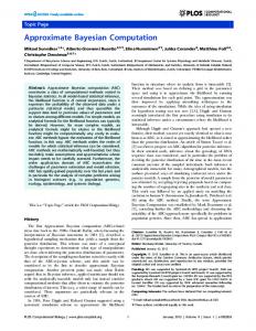
The call to the inla() function is not changed. The estimated posterior mean and quantiles of the non-linear effect of age is plotted in Figure 2a and the nonlinearity of the age effect is clear. The improvement obtained by using a more flexible model for the effect of the age covariate can be seen also from the decreased value of the DIC in Table 2. This second model results also to be more powerful as a prediction tool, as indicated by the decreased value of the logarithmic score in Table 2. Also for this model the predictive quantities are computed without problems and the pit distribution is close to uniform. The estimates of the other parameters in the model is reported in Table 1, the estimated spatial effects are similar to that in MOD1 and is not reported here. Results are similar to those obtained using BayesX, a program which performs a MCMC study [13]. As an alternative hypothesis to explain spatial variability one could imagine that the effect of one covariate, for example the mother’s bmi, although being linear has a different slope for different regions. Again we assume this spatial variability to be

12

Sara Martino and H˚avard Rue

Table 2 DIC value and logarithmic score for the three model in the Zambia example. MOD2

MOD3

mean of the deviance deviance of the mean effective number of parameters DIC

13030.66 12991.61 39.04 13069.71

12679.90 12630.89 49.01 12728.92

12672.22 12610.68 61.53 12733.76

log Score

1.357

1.313

1.314

0.5

1.0

MOD1

0.0

0.04 0.03 0.03 0.02 0.01 0.01 0

0

10

20

30

40

50

60

Age

Fig. 2a Estimated effect of age (posterior mean together with 2.5% and 97.5% quantiles) using MOD2

Fig. 2b Posterior mean for the space-varying regression coefficient in MOD3

smooth. This kind of models are known as space-varying regression models [10]. Using the notation in equation (2) the model (MOD3) can be written as:

ηi = µ + zTi β + f1 (agei ) + bmii f2 (si )

(7)

We assume here that the whole spatial variability is explained by the space varying regression parameter so that no other spatial effect is needed. Moreover we assume the age covariate to have a non linear effect. The model for f1 (·) is as in MOD2 while for f2 (·) we assume "besag" model, this time the sum-to-zero constraint is not necessary since there are no identifiability problem. Here the bmi covariate simply act as a known weight for the IGMRF f2 (·). The INLA specification of the model is as follows: >formula = hazstd ˜ edu1 + edu2 + tpr + sex + + f(agc, model="rw2") + + f(district, bmi, model="besag", + graph.file="zambia.graph", + constr=FALSE)

Case Studies in Bayesian Computation using INLA

13

The order of district and bmi in the second of the f() functions of the formula above is important since arguments are matched by position: the first argument is always the latent field and the second is always the weights. Note, moreover, that the sum-to-zero constraint has to be explicitly removed since, as said before, is is default for all intrinsic model. The resulting estimates for the space varying regression parameter are displayed in Figure 2b The computing time (using the default CCD strategy) goes from a minimum of 9 seconds for MOD1 to a maximum of 14 seconds for MOD2.

5.3 A simple example of survival data analysis Our last example comes from the survival analysis literature. A typical setting in survival analysis is that we observe the time point t at which the death of a patient occurs. Patients may leave the study (for some reason) before they die. In this case the survival time is said to be right censored, and t refers to the time point when the patient left the study. The indicator variable δ is used to indicate whether t refers to the death of the patient (δ = 1) or to a censoring event (δ = 0). The key quantity in modeling the probability distribution of t is the hazard function h(t), which measures the instantaneous death rate at time t. We also define the cumulative R hazard function H(t) = 0t h(s) ds, implicitly assuming that the study started at time t = 0. A different starting time can also be considered and it is usually referred to as truncation time. The log-likelihood contribution from one patient is δ log(h(t)) − H(t). A commonly used model for h(t) is Cox’s proportional hazard model [4], in which the hazard rate for the ith patient is assumed to be on the form hi (t) = h0 (t) exp(ηi ),

i = 1, . . . , n.

Here, h0 (t) is the baseline hazard function (common to all patients) and ηi is a linear predictor. In this example we shall assume that the baseline hazard belongs to the Weibull family: h0 (t) = α t α −1 for α > 0. In [17] this model is used to analyze a data set on times to kidney infection for a set of nd = 38 patients. The data set contains two observations per patient (the time to first and second recurrence of infection). In addition there are three covariates: age (continuous), sex (dichotomous) and type of disease (categorical, four levels), and an individual specific random effect (vn: ID), often named frailty: ui ∼ N(0, τ −1 ). Thus, the linear predictor becomes

ηi = β0 + βsex sexi + βage agei + βD xi + ui

(8)

where βD = (β2 , β3 , β4 ) and xi is a dummy vector coding for the disease type. Here we used a corner-point constraint imposing β1 = 0. Fitting a survival model using INLA is done using the following commands: >formula = inla.surv(time,event) ˜ age + sex + dis2 + dis3 +

14

Sara Martino and H˚avard Rue + dis4 + f(ID, model="iid") >mod = inla(formula, family="weibull", data=Kidney)

Note that the function inla.surv() is needed to define the response variable of a survival model. This functions is used to define different censoring schemes such as right, left or interval censoring plus, possibly, truncation times. Including more complex effects in model (8) such as, for example, smooth effects of covariates or spatial effects can be done in exactly the same way as for the previous examples. Posterior means and standard deviations, together with quantiles, for the model parameters are shown in Table 3 and are similar to those obtained by Gibbs sampling via WinBUGS and by maximum likelihood. Fitting the model took less than 2 seconds. Table 3 Posterior mean, standard deviation and quantiles for the parameters in the survival data example

β0 βage βsex β2 β3 β4 α τ

mean

sd

2.5%quant

97.5%quant

-4.809 0.003 -2.071 0.155 0.679 -1.096 1.243 2.365

0.954 0.016 0.535 0.591 0.595 0.863 0.151 1.647

-6.77 -0.028 -3.180 -1.007 -0.467 -2.813 0.970 0.586

-3.103 0.036 -1.076 1.346 1.900 0.611 1.560 6.976

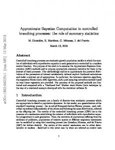
The inla() function computes the posterior marginals for the hyperparameters θ = (α , τ ) using only few points in the θ space (CCD strategy). As noted in Section 3 this might be not accurate enough. The function inla.hyperpar(), which takes as input the output of inla(), recomputes the marginals for the hyperparameters in a more accurate way, using a grid integration: > hyperpar = inla.hyperpar(mod)

In cases where the dimension m of θ is large, computing posterior marginals using inla.hyperpar() can be time consuming. In this case, being m = 2, recomputing marginals for θ took less than 3 seconds. Figure 3 shows the two approximations for the hyperparameters in model 8. For the current example there is no special improvement coming from using the more accurate approximation computed by inla.hyperpar(). The INLA library can also deal with exponential models for the baseline function h0 (t). Semi-parametric models for h0 (t) such as piecewise log-constant are, at the moment of writing, under study.

15

0.0

0.0

0.5

0.1

1.0

0.2

1.5

0.3

2.0

0.4

2.5

Case Studies in Bayesian Computation using INLA

1.0

1.2

1.4

1.6

1.8

0

2

4

6

8

Fig. 3 Estimate of the posterior marginals for θ basic estimation (solid line) and improved one (dashed line). Left: posterior marginals for α . Right: posterior marginal for τ .

6 Discussion As shown in this paper INLA is a powerful inferential tool for latent Gaussian models. The computational core of the inla program treats any kind of latent field in the same way thus behaving as a black-box. The available R interface INLA, can easily be handled by the user to obtain fast and reliable estimates. The large series of different options both for the approximations of the posterior marginals of the latent field, and for the exploration of the hyperparameter space may generate confusion in the novice user. On the other side, the default choices in the INLA library, offer usually a good starting point for the analysis. The INLA library computes also quantities useful for model comparison, a feature that becomes important when the computational speed gives the possibility to fit several models to the same data set. The INLA library contains also functions to process the posterior marginals obtained by the inla() function, so that it is possible to compute quantiles, percentiles or expectations of functions of the original random variable. Sampling from such posterior marginals is also possible.

References 1. Banerjee, S., Carlin, B., Gelfand, A.: Hierarchical Modeling and Analysis for Spatial Data. Chapman & Hall (2004) 2. Besag, J., York, J., Mollie, A.: Bayesian image restoration with two application in spatial statistics. Annals of the Institute in Mathematical Statistics 43(1), 1-59. (1991)

16

Sara Martino and H˚avard Rue

3. Breslow, N.E. and Clayton D.G.: Approximate inference for Generalized Linear Mixed models. Journal of the American Statistical Association, 88, 9-25. (1993) 4. Cox, D.R. : Regression models and life-tables. Journal of the Royal Statistical Society, Series B, 34, 187-220 (1972) 5. Crowder, M.J. :Beta-Binomial ANOVA for Proportions. Applied Statistics, 27, 34-37. (1978) 6. Czado, C., Gneiting, T. and Held, L.: Predictive model assessment for count data. Biometrics 65, 1254-1261 (2009) 7. Eidsvik, J., Martino, S., Rue, H.: Approximate Bayesian Inference in spatial generalized linerar mixed models. Scandinavian Journal of Statistics, 36 .(2009) 8. Fahrmeir, L., Tutz, G.: Multivariate Statistical Modeling Based on Generalized Linear Models. Springer Verlag, Berlin (2001) 9. Fong, Y., Rue H., and Wakefield J.: Bayesian inference for Generalized Linear Mixed Models, Biostatistics, doi:10.1093/biostatistics/kxp053 (2009) 10. Gamerman, D., Moreira, A. and Rue, H.:Space-varying regression models: specifications and simulation. Computational Statistics & Data Analysis 42 513533 (2003) 11. Gneiting, T., Raftery, A.E.: Strictly proper scoring rules, prediction and estimation. Journal of American Statistical Association, Series B, 102, 359-378. (2007) 12. Held, L., Schrodle, B., Rue, H.: Posterior and cross-validatory predictive checks: A comparison of MCMC and INLA. In: Kneib, T., Tuts, G. (eds) Statistical Modeling and Regression structures - Festschrift in Honour of Ludwig Fahrmeir, Springer (2010) 13. Kneib, T., Lang, S. and Brezger, A.: Bayesian semiparametric regression based on MCMC techniques: A tutorial (2004) 14. Kandala, N. B., Lang, S., Klasen, S. and Fahrmeir, L.: Semiparametric Analysis of the SocioDemographic and Spatial Determinants of Undernutrition in Two African Countries. Research in Official Statistics, 1, 81100. (2001) 15. Lunn, D.J., Thomas, A., Best, N., and Spiegelhalter, D.: WinBUGS – a Bayesian modelling framework: concepts, structure, and extensibility. Statistics and Computing, 10:325–337, (2000) 16. Martino, S., Rue, H.: Implementing Approximate Bayesian inference using Integrated Nested Laplace Approximation: A manual for the INLA program. Technical report, Norwegian University of Science and Technology, Trondheim. 17. McGilchrist C.A., Aisbett C.W.: Regression with frailty in survival analysis, Biometrics 47(2) 461-466, (1991). 18. Rue, H., Held, L.: Gaussian Markov Random Fields: Theory and Applications. Vol. 104 of Monographs on Statistics and Applied Probability, Chapman&Hall, London (2005) 19. Rue H., Martino S.: Approximate Bayesian Inference for Hierarchical Gaussian Markov Random Fields Models. Journal of Statistical Planning and Inference, 137 3177-3192(2007) 20. Rue, H., Martino, S., Chopin, N.: Approximate Bayesian Inference for Latent Gaussian Models Using Integrated Nested Laplace Approximations (with discussion). Journal of the Royal Statistical Society, Series B 71, 319-392 (2009) 21. Spiegelhalter, D., Best, N., Bradley, P., van der Linde, A.: Bayesian measure of model complexity and fit (with discussion). Journal of the Royal Statistical Society, Series B, 64,4, 583639. (2002) 22. Tierney, L. and Kadane, J. B.: Accurate approximations for posterior moments and marginal densities. J. Am. Statist. Ass., 81, 82-86. (1986)