K. Santhi Sree, Ph.D. ... distance-based outlier detection approaches (an exact and an ... detection of outliers within a state set, in both the incremental ... To deal with multi dimensional data it requires special ... Fuzzy and Cosine Manhattan, Minkowski similarity .... from each state set a cell-based approach [11] is used. This.
International Journal of Computer Applications (0975 – 8887) Volume 112 – No. 8, February 2015
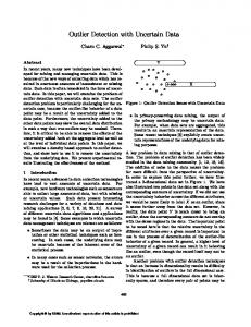
Case Study: Outlier Detection on Sequential Data K. Anusha
S. Manoj Kumar
K. Santhi Sree, Ph.D.
M. Tech Student, School of IT JNTUH, Hyderabad
M. Tech student, School of IT JNTUH, Hyderabad
Professor, School of IT JNTUH, Hyderabad
ABSTRACT Time series data streams are common in wireless sensor networks in nowadays. This type of data is having uncertainty due to the limitation of the measuring equipments or other sources of corrupting noise, leading to uncertain data. As uncertain streaming data is continuously generated, mining algorithms should be able to analyze the uncertain data. To detect the outliers in this project we propose two continuous distance-based outlier detection approaches (an exact and an approximate) are proposed for uncertain time series data streams. These two algorithms are implemented based on the cell based approach. These two approaches can be applied on uncertain objects. A set of uncertain objects at particular time stamp is called state set. As the duration between the two time stamps is very less to detect the outliers we use the incremental approach (use the results obtained from the previous state set to detect outliers in the current state set). An approximate incremental outlier detection approach is proposed to further reduce the cost of incremental outlier detection. Cell based algorithm is employed for the efficient detection of outliers within a state set, in both the incremental algorithms. To show the efficiency of the proposed approaches synthetic and real datasets are used.
Keywords Clustering; Outlier detection; Cell-Based Approach; Grid-File indexing; Incremental Outlier Approach;
1. INTRODUCTION 1.1 Clustering Clustering is a data mining technique that categories the data into multiple groups, called as clusters. The main property of data clustering is inter cluster similarity has to be maximized and intra-cluster similarity has to be minimized. All the patterns that lie in one cluster are similar to one another and dissimilar when compared to clusters in the other clusters .i.e. the distance between the patterns that lie in one cluster is less and similarity between patterns that lie in two different clusters is more. The various types of clustering techniques are partitioning algorithms, hierarchical algorithms, density- based, grid based and model- based algorithms. K-means and K-mediods are partitioning algorithms , Agglomerative and Divisive are Hierarchical clustering , Agglomerative starts with a multiple singleton clusters and are grouped recursively to form a single cluster. Divisive clustering start with a single cluster and segregates into multiple singleton clusters. The various components of clustering are Feature extraction, Intercluster similarity, grouping into clusters. Initially the data is collected and the sequences are converted into some intermediate representation and inter cluster similarity is calculated and applying any of the clustering techniques the data is categorized into groups [12].
Fig 1. Clustering Types
1.2 Outlier Detection An outlier is an observation point which differs from other observations in a group. Outliers are also referred as abnormalities, discordant or anomalies in the data mining. Outliers can be caused by errors in data, changes in system
behavior or even instrument error. Outlier mining is applicable in many applications like network intrusion detection, fraud detection, detection of unexpected entries in database and etc. The outlier mining problem can be identified as two problems:
29
International Journal of Computer Applications (0975 – 8887) Volume 112 – No. 8, February 2015 1.
Define the inconsistent data in given data set.
2. RELATED WORK
2.
Find the appropriate method to mine outliers efficiently.
The problem of outlier detection has been classified into statistical approaches, depth-based approaches, deviationbased approaches, distance-based approaches, density-based approaches and high-dimensional approaches by [8]. Distance-based outlier detection approach on static data was introduced by Knorr et al. in [3]. They defined a data object o to be an outlier if at most threshold θ objects are within Ddistance of o. [10] formulated distance-based outliers as the data objects whose distance to their κth nearest neighbor is largest. Angiulli et al. in [4] gave a slightly different definition of outliers than [10] by considering the average distance to their k nearest neighbors. Beside these, there are some works on the detection of distance-based outliers over data streams including [8], [5]. These works are based on the Knorr et al.[3] definition of outliers. Among these works, the incremental algorithm proposed in [5] is closest to our work. However, all these works deal with deterministic data and cannot handle uncertain data.
Finding outliers in time series data becomes tricky because they may be hidden in trend, seasonal or other cyclic changes. To deal with multi dimensional data it requires special consideration for categorical (i.e., nonnumeric) data.
1.3 Euclidean Similarity Measure Similarity measure is used to find out how similar any two sequences are. In the history many similarity measures exist, and they are Euclidean similarity , Jaccard similarity, Fuzzy and Cosine Manhattan, Minkowski similarity measures. These similarity measures are vector based similarity measures. Euclidean distance measure is a popularly used similarity/ distance measure for vector spaces for two sequences S1 and S2 in an N- dimensional space. It is defined as the square root of the sum of the corresponding dimensions of the vector. The Euclidean distance between sequences S1= (S11, S12... S1n) and S2= (S21, S22,..., Sn) is defined as
Recently, a lot of research has focused on managing, querying and mining of sequential datasets [2], [1]. The problem of outlier detection on sequential datasets was first studied by Aggarwal et al. [2]. According to them, an uncertain object o 𝑠𝑖𝑚 𝑆1 , 𝑆2 is a density-based (δ, η) outlier, if the probability of existence 2 2 2 = (𝑆1 1 − 𝑆2 1 ) + (𝑆1 2 − 𝑆2 2 ) + ⋯ + (𝑆1 𝑛 − 𝑆2 𝑛 ) of o in some subspace with density at least η is less than δ. However, their work was given for static data and cannot handle continuous data. In [1], Wang et al. proposed an outlier 𝑛 detection approach for probabilistic data streams. However, their work focuses on the tuple-level uncertainty. In contrast, = (𝑆1 𝑖 − 𝑆2 𝑖 )2 in this paper, attribute level uncertainty is considered, i.e., the 𝑖=1 uncertainty lies in the measurements obtained from sensors. Direct application of Euclidean distance measure across sequences is not possible. Sequences have to be first converted into n-dimensional vector representations. Over these transformed vectors Euclidean distance measure is applied to find the distance between the two. For example consider two sequences S1={a,b,a,c,a,a} and S2={b,a,b,b,b,b}. The transformed vectors of S1 and S2 are {1,1,1} and {1,1,0} respectively and the Euclidean similarity measure is now defined as 1. The two sequences seem to be dissimilar.
1.4 Sequential Data Sequential data is a sequence of data points. This data is usually collected at regular intervals of time. This data is used in mathematical finance, weather forecasting, earthquake prediction and etc. Time series data is a sequence of data points, consisting of successive measurements over a time interval. Time series analysis aims to describe and summarize time series data and make forecasts. Time series forecasting is used to predict the future values based on previous values. This could be done with regression analysis (method of prediction). This method of prediction usually based on statistical interpretation of time series properties in the time domain.
3. PROPOSED WORK Data streams are the sequence of objects states generated over time. The states of all objects are generated synchronously and the set of states at particular time stamp is called state set. In the naïve approach (i.e., Nested loop) to detect the outlier's number of distance functions evaluations is more. So it requires lot of computational time to detect the outliers even for small data sets. To detect the outliers on sequential data from each state set a cell-based approach [11] is used. This proposed approach can reduce significantly the number of distance functions evaluations. Initially data objects can be mapped to a cell grid structure. Identify the bounds of a cell or cell layer to prune the outliers without evaluating the distance functions for the objects. The structure of a cell bounds as follows:
Time series data can be displayed in scatter plot. Vertical axis can represent the series value X. Horizontal axis can represent the time t where time is an independent variable. There are two kinds of time series data. (i)Continuous, it is an observation which is recorded at every instant of time. This observation can be represented as X at time t, X(t). (ii) Discrete, it is an observation which is collected at regular spaced intervals, we denote this as Xt.
Fig 2. Structure of cell bounds
30
International Journal of Computer Applications (0975 – 8887) Volume 112 – No. 8, February 2015 Then prunes objects by identifying the cells which contains only outliers or non-outliers based on the bounds on number of D-neighbors. In the process of pruning, some of the cells are neither pruned as non- outliers nor as outlier cells (undecided). To prune those objects cells use the nested loop approach. This distance function requires lot of computational time for initial pruning. So use the grid structure as Grid- file index to reduce the additional indexing cost for the farther objects. Hence Grid File indexing [9] for un-pruned objects reduces the overall cost of computations. In the cell based approach some outliers can be obtained at each time stamp. As the duration between the two time stamps is very low the objects may not change in this short time. To reduce the unnecessary computations at each time stamp and the continuous arrival of data to find the outliers on sequential
data use the incremental outlier detection approach. In this incremental approach [11] previous state set (si-1) results can be used to find the outliers of current state set (si) at time stamp ti. This approach reduces the lot of computation time.
Architecture
Collect the objects from each state set at a particular time stamp.
Map the collected objects to the cell grid structure.
Prune the objects by finding the outliers and non outliers.
Use the Grid file indexing to prune the un-pruned objects which are undecided.
Fig 3. Overall Architecture Algorithm 1: Cell Based Approach. Input: database GDB, distance d, percentage p, standard deviation σ Output: Distance Based Outliers on Sequential Data. Method: 1.
Compute and store cell bounds into lookup table using cell length l and maximum distance between any two objects;
2.
Initialize the count of each cell in grid;
3.
Map the database objects to appropriate cells;
4.
calculate the threshold value;
5.
Prune the outlier and non-outlier cells using cell layers’ bounds i.e,. Calculate minimum and maximum contribution of cell Ci using upper and lower bounds respectively of 0 to jth neighboring cell layers of Ci;
6.
7.
Un-pruned objects are pruned using Grid File Index i.e., if object is not pruned as outlier or non-outlier cell then find out EVO ( expected value of object O); The resultant object mark as outlier;
3.1 Incremental Outlier Processing This approach process only the state change (SC) objects or which are affected by state change (SC) objects. This approach targets all the state sets except initial state set (S1). All the objects in the S1 need to be processed by using the cell- based approach. The objects in the remaining state sets can be processed as follows: Case [1]: when object Op moved to different cell it affects the cell bounds of all the cells [11]. 𝑗 −1
𝑗
𝑗 −1
𝑗
𝑂𝑝 ∈ 𝐶𝑥1,𝑥2 , 𝑂𝑝 ∈ 𝐶𝑥1,𝑥2 , 𝐶𝑥1,𝑥2 ≠ 𝐶𝑥1,𝑥2 Case [2]: When object Op moved within a cell it affects the un-pruned objects in the G [11]. 𝑗 −1
𝑗
𝑗 −1
𝑗
𝑂𝑝 ∈ 𝐶𝑥1,𝑥2 , 𝑂𝑝 ∈ 𝐶𝑥1,𝑥2 , 𝐶𝑥1,𝑥2 ˭ 𝐶𝑥1,𝑥2 The cells which are affected by the state change (SC) objects called target cells. Type A: Cells containing SC-objects which have moved to or from another cell at time tj. Type B: L1 and RD+wσ neighboring cells of Type A cells, except those classified as Type A. Type C: Un-pruned cells of the grid G. Type C cells may include Type A and B cells.
31
International Journal of Computer Applications (0975 – 8887) Volume 112 – No. 8, February 2015 10. Until no un-pruned cell found;
Algorithm 2: Incremental Outlier Approach Input: Sj, G, θ
11. Return O;
Output: Set of distance-based outliers O.
4. EXPERIMENTAL DATA
Method: 1.
Identifying state change objects;
2.
Repeat;
3.
If object Oi moved to different cell add Oi to appropriate cell CJ;
4.
Until no new object found in Si;
5.
Label each Cj ∈ G C, if Cj is non-empty, un-pruned and not labeled A or B;
6.
Process the target cells of types A, B and C;
7.
Repeat;
8.
If any object Oi un-pruned in the cell CJ compute the # D- neighbors of Oi.;
9.
If the #D-neighbors is less than threshold add Oi to the outlier O;
As for real-world data, use met office weather (MOW) forecast data [7]. To conduct the experiments on real data, a two dimensional subset of MOW data is used in Table1. It consists of screen and feels like temperature forecast values. Consecutive forecasts are used as data stream in these experiments. State change objects ratio for the MOW dataset depends on the number of objects changing states between two forecasts. 1.
The first two rows contain the British National Grid easting and northing of the grid point (i.e. the centre point of a 5 x 5 km grid cell).
2.
The easting and northing are for the centre of the selected grid cell - they can be used to locate the grid cell within the time series data files.
3.
Subsequent columns contain values of the climate variable for a monthly or annual time series.
Table 1. Experimental data (MOW) Easting
Northing
Jan-07
Feb-07
Mar-07
Apr-07
May-07
Jun-07
462500
1217500
6.95
6.71
8.34
10.2
10.81
13.05
457500
1212500
6.76
6.63
8.47
10.62
11.17
13.43
462500
1212500
6.85
6.67
8.35
10.3
10.97
13.15
457500
1207500
6.91
6.87
8.79
11.03
11.62
13.83
462500
1207500
7.04
6.7
8.42
10.48
10.86
13.07
447500
1202500
7
6.73
8.71
11.17
11.21
13.53
452500
1202500
6.41
6.19
8.14
10.58
10.91
13.19
457500
1202500
6.79
6.69
8.63
10.95
11.47
13.67
462500
1202500
7.08
6.92
8.7
10.81
11.4
13.52
447500
1197500
6.87
6.55
8.51
11.02
11.11
13.37
452500
1197500
6.93
6.79
8.81
11.3
11.63
13.85
432500
1192500
7.44
6.5
8.19
10.64
9.99
12.28
437500
1192500
6.99
6.12
7.81
10.25
9.86
12.08
442500
1192500
7.39
6.79
8.63
11.11
10.95
13.14
447500
1192500
6.93
6.47
8.34
10.8
10.91
13.07
452500
1192500
6.86
6.58
8.5
10.95
11.3
13.44
457500
1192500
7.1
6.95
8.83
11.15
11.67
13.75
32
International Journal of Computer Applications (0975 – 8887) Volume 112 – No. 8, February 2015 462500
1192500
6.62
6.29
7.83
9.82
10.46
12.42
432500
1187500
6.69
5.55
7.16
9.64
9.12
11.36
437500
1187500
7.19
6.24
7.92
10.37
10.04
12.19
447500
1187500
6.64
5.82
7.4
9.68
9.77
11.78
452500
1187500
6.84
6.25
7.87
10.09
10.38
12.36
462500
1187500
7.23
6.82
8.23
10.07
10.65
12.49
422500
1182500
7.7
6.6
8.33
10.94
10.01
12.42
427500
1182500
7.15
6.04
7.78
10.38
9.73
12.06
month i.e., if there are 10 samples collected in a month it is aggregate of those 10 samples. Collect the synthesized data which is equivalent to the experimental data. Table 2. Similarity measures
From this experimental data we consider only 10 samples for experiment. The each cell contains aggregate value of each
Similarity measure
T1
T2
T3
T4
T5
T6
T7
T8
T9
T10
T1
0
2.44
2.23
2.44
1.73
1.41
2.23
2
2.44
2.23
T2
2.44
0
2.23
1.41
2.23
2.23
2.23
2.23
2
2.44
T3
2.23
2.23
0
2.23
2
1.41
1.41
1
2.23
1.73
T4
2.44
1.41
2.23
0
2.23
2.64
2
2
2.44
2
T5
1.73
2.23
2
2.23
0
2
2.44
2
2.64
2.64
T6
1.41
2.23
1.41
2.64
2
2
1.73
2.44
2.44
T7
2.23
2.23
1.41
2
2.44
2
1
2.44
1
T8
2
2.23
1
2
2
1.73
1
0
2.44
1.41
T9
2.44
2
2.23
2.44
2.64
2.44
2.44
2.44
0
2.44
T10
2.23
2.44
1.73
2
2.64
2.44
1
1.41
2.44
0
Clusters formed for 200 samples collected from internet source.
C1={ T1,T3,T5,T6,T8,T7,10}
C2={T2}
C3={T4}
C4={T3,T5,T6,T8}
C5={T1,T5,T6,T7,T8,T9}
C6={T1,T3,T6}
C7={T1,T3,T5,T7,T8}
C8={T3,T6,T8,T10}
C9={NOISE}
0
0
C10={NOISE}
C11={T1,T3,T4,T6,T7}
C12={T3,T7,T8}
Consider arbitrarily 10 records of web transactions. The transactions are converted to vector representation, and a 10 X 10 similarity matrix is computed using Euclidean. In the step two after applying clustering technique, Clusters formed are 12. Table3 12 X 12 matrix where rows and columns indicate the clusters Ci ={C1, C2, C3, C4, C5, C6, C7, C8, C9, C10, C11, C12} which shows the inter cluster distance using Euclidean distance measure. For example, the inter cluster distance (C1, C2) =0.15. and inter cluster distance between the clusters (C3,C12)=0.2.That is the patterns lying in the cluster C3 are more dissimilar when compared to the patterns lying in the cluster C12.
33
International Journal of Computer Applications (0975 – 8887) Volume 112 – No. 8, February 2015 Table 3. Inter Cluster Similarity Ci X Ci
C1
C2
C3
C4
C5
C6
C7
C8
C9
C10
C11
C12
C1
0
0.15
0.16
0.16
0.16
0.16
0.17
0.17
0.18
0.18
0.19
0.19
C2
0.15
0
0.13
0.13
0.14
0.13
0.13
0.14
0.15
0.16
0.17
0.18
C3
0.16
0.13
0
0.12
0.14
0.15
0.15
0.15
0.16
0.17
0.19
0.21
C4
0.16
0.13
0.12
0
0.18
0.18
0.18
0.19
0.19
0.19
0.21
0.21
C5
0.16
0.14
0.14
0.18
0
0.16
0.16
0.16
0.17
0.17
0.18
0.18
C6
0.16
0.13
0.15
0.18
0.16
0
0.16
0.17
0.18
0.21
0.22
0.23
C7
0.17
0.13
0.15
0.18
0.16
0.16
0
0.21
0.21
0.22
0.23
0.24
C8
0.17
0.14
0.15
0.19
0.16
0.17
0.21
0
0.18
0.18
0.18
0.18
C9
0.18
0.15
0.16
0.19
0.17
0.18
0.21
0.18
0
0.21
0.21
0.22
C10
0.18
0.16
0.17
0.19
0.17
0.21
0.22
0.18
0.21
0
0.22
0.23
C11
0.19
0.17
0.19
0.21
0.18
0.22
0.23
0.18
0.21
0.22
0
0.18
C12
0.19
0.18
0.21
0.21
0.18
0.23
0.24
0.18
0.22
0.23
0.18
0
Using incremental outlier approach the outliers deleted are
C1= { T1,T3,T5,T6,T8,T7,10}
C2= {T2}
C3= {T4}
C9= {NOISE}
C10= {NOISE}
C12= {T3, T7,T8}
Next the inter cluster similarity, intra clusters are calculated that demonstrate the data varies from time to time in a sequential data. Table 4. Intra Clusters based on Euclidean
Intra cluster
C1
C2
C3
C4
C5
C6
C7
C8
C9
C10
C11
C12
Euclidean
2.64
2.38
1.94
2.04
2.24
1.94
2.47
2.42
2.5
2.34
2.31
2.31
5. CONCLUSION
6. REFERENCES
In this work, Distance-based outlier detection approach is proposed to detect the outliers for sequential data streams. The proposed approaches are based on the incremental processing of the state change objects. To detect the outliers on continuous arrival of data incremental algorithm is proposed. This approach uses the results obtained from the previous state set to efficiently detect outliers in the current state set. The incremental algorithms process the objects which are affected by the change in objects states. Use a cell based algorithm for the efficient detection of outliers within a state set, in the incremental algorithm. This can be done by pruning majority of outliers and non-outliers cells. Grid-file indexing is utilized to reduce the additional indexing cost for farther objects in the cell. This grid file indexing further reduces the overall cost of computation time required for the cell based algorithm. An extensive empirical study on synthetic and real datasets demonstrates the efficiency of the proposed approach. In the future, the work can be extended for high-dimensional data, data sparsity in high dimensional data. To determine the outliers in sparsed high dimensional data, density distributions of projections can be used.
[1] B. Wang, G. Xiao, H. Yu, and X. Yang, “Distance-based outlier detection on uncertain data,” in CIT, 2009. [2] C. C. Aggarwal and P. S. Yu, “Outlier Detection with Uncertain Data,” in SDM, 2008. [3] E. M. Knorr, R. T. Ng, and V. Tucakov, “Distance-based outliers: Algorithms and applications,” VLDB J., vol. 8(3-4), pp(237–253), 2000. [4] F. Angiulli and C. Pizzuti, “Fast outlier detection in high dimensional spaces,” in Principles of Data Mining and Knowledge Discovery, pp. 15–27,2002. [5] K. Ishida and H. Kitagawa, “Detecting current outliers: Cont. outlier detect. over time-series data streams,” in DEXA, 2008. [6] Kriegel, H.-P., Kr¨oger, P., Zimek, A.: Outlier Detection Techniques. Tutorial at 16th ACM SIGKDD Conference 2010. [7] “Met office weather data,” http://data.gov.uk/data, 2013,
34
International Journal of Computer Applications (0975 – 8887) Volume 112 – No. 8, February 2015 [Online; accessed 03-September-2013]. [8] M. Kontaki, A. Gounaris, A. Papadopoulos, K. Tsichlas, and Y. Manolopoulos, “Continuous monitoring of distance-based outliers over data streams,” in ICDE, 2011. [9] Nievergelt, J., Hinterberger, H., Sevick, K.C.: The Grid File: An Adaptable, Symmetric multikey File Structure. ACM Transaction on Database Systems 1984. [10] S. Ramaswamy, R. Rastogi, and K. Shim, “an efficient algorithm for mining outliers from large data sets,”
IJCATM : www.ijcaonline.org
SIGMOD Rec., vol. 29(2), 2000. [11] Salman Ahmed Shaikh and Hiroyuki Kitagawa “Continuous Outlier Detection on Uncertain Data Streams” in ISSNIP, 2014. [12] http://www.cs.gsu.edu/~wkim/index_files/SurveyParallel Clustering.html. [13] Y. Tao, X. Xiao, and R. Cheng, “Range search on multidimensional uncertain data,” ACM Trans. Database Syst., vol. 32(3), 2007.
35