ABSTRACT ... many applications, such as fraud detection for credit card [1], cy- ber security ... clustering algorithm, while maintaining a parameter regarding the.
Parameterless Outlier Detection in Data Streams Alice Marascu and Florent Masseglia INRIA AxIS Project-Team 2004 route des lucioles - BP 93
{first.last}@sophia.inria.fr
ABSTRACT Outlyingness is a subjective concept relying on the isolation level of a (set of) record(s). Clustering-based outlier detection is a field that aims to cluster data and to detect outliers depending on their characteristics (small, tight and/or dense clusters might be considered as outliers). Existing methods require a parameter standing for the “level of outlyingness”, such as the maximum size or a percentage of small clusters, in order to build the set of outliers. Unfortunately, manually setting this parameter in a streaming environment should not be possible, given the fast time response usually needed. In this paper we propose W OD, a method that separates outliers from clusters thanks to a natural and effective principle. The main advantages of W OD are its ability to automatically adjust to any clustering result and to be parameterless.
Categories and Subject Descriptors H.4 [Information Systems Applications]: Miscellaneous
Keywords Data Streams, Outliers, Parameterless
1.
INTRODUCTION
Clustering is a major topic of data mining that aims to separate objects into groups (or clusters) according to their similarity. The first goal of clustering was to provide patterns representing the majority of data. In contrast, outlier detection aims to discover highly unlikely data. This is an important topic of data mining since it has many applications, such as fraud detection for credit card [1], cyber security [4] or safety of critical systems [6]. Actually, outliers might be indicative of suspicious data such as skewed or erroneous values, entry mistakes or malicious behaviours. A malicious behaviour can be detected as an outlier in datasets such as transactions in a credit card database or records of usage on a web site. To the best of our knowledge, outlier detection always relies on a parameter, given by the end-user and standing for a “degree of outlyingness” above which records are considered as atypical. For instance, in [11], a distance-based outlier is an object such that
Permission to make digital or hard copies of all or part of this work for personal or classroom use is granted without fee provided that copies are not made or distributed for profit or commercial advantage and that copies bear this notice and the full citation on the first page. To copy otherwise, to republish, to post on servers or to redistribute to lists, requires prior specific permission and/or a fee. SAC’09 March 8-12, 2009, Honolulu, Hawaii, U.S.A. Copyright 2009 ACM 978-1-60558-166-8/09/03 ...$5.00.
a user-defined fraction of dataset objects have a distance of more than a user-defined minimum distance from that object. In [5], the authors propose a nonparametric clustering process and the detection of outliers requires a user defined value k corresponding to the top-k desired outliers. In this paper we propose W OD (Wavelet-based Outlier Detection), a parameterless method intending to automatically extract outliers from the results of a clustering step. In contrast to previous work, our goal is to find the best division of a distribution and to automatically separate values into two sets corresponding to clusters on the one hand and outliers on the other hand. The tail of the distribution is found thanks to a wavelet technique and does not depend on any user threshold. Our method fits any distribution depending on any characteristic such as distances between objects [11], objects’ density [2, 14] or clusters’ size [8]. Our framework involves clustering-based outlier detection in data streams. Clustering-based detection of outliers aims to find objects that do not follow the same model as the rest of the data depending on the clusters’ size or tightness [8, 17, 5]. This framework will allow us to illustrate our proposal with one of the possible characteristics observed for building a distribution of objects (i.e. clusters’ size). The choice of data streams is motivated by the specific constraints of this domain. In a data stream environment, data are generated at a very high rate and it is not possible to perform blocking operations. In this context, requesting a parameter such as k, for top-k outliers, or x, a percentage of small clusters, should be prohibited. First, because the user doesn’t have enough time to try different values of these parameters for each period of analysis on the stream. Secondly, because a permanent value may be adapted to one period of the stream but it is highly likely to be wrong on the next periods (the data distribution will change, as well as the number or percentage of outliers). For these reasons, detecting outliers should not depend on any parameter and should be adaptive in order to keep the best accuracy all along the stream. This paper is organized as follows. Section 2 gives an overview of existing works in outlier detection and Section 3 gives a formal definition of our problem. Our method relies on a clustering step described in Section 4. Section 5 gives the details of W OD and its principle for separating outliers from clusters. Section 6 shows the advantages of W OD through a set of experiments on real Web usage data and Section 7 gives our conclusion.
2.
RELATED WORKS
In this paper, we focus on clustering-based outlier detection algorithms [11, 16, 9, 7, 14]. Such techniques rely on the assumption that normal points belong to large clusters while outliers either do not belong to any cluster [11, 16] or form very small and tight clusters [8, 17, 5]. In other words, outlier detection consists in identi-
fying among data those that are far from being significant clusters. Depending on the approach, the number of parameters required to run the algorithm can be high and will lead to different outliers. To avoid this, some works return a ranked list of potential outliers and limit the number of parameters to be specified [16, 9, 5]. Let us note that [5] proposes to reduce or to avoid given parameter to the clustering algorithm, while maintaining a parameter regarding the outliers: n the number of required outliers. In this paper, we aim to detect outliers on the basis of clusters characteristics only. Among these characteristics, we have selected the clusters’ size. A distribution of the clusters’ size combined with our wavelet approach allows cutting the clusters set into two sub-sets, basically corresponding to “big” and “small” clusters. This method would also cut down this set with regard to other characteristics, such as clusters tightness or their number of neighbors (density) for instance.
3.
PROBLEM STATEMENT
We instantiate W OD on streaming usage data of a Web site. We need to define a navigation sequence as the series of URLs requested by a user. D EFINITION 1. Let I = i1 , i2 , ..., in be a set of items. Let X = i1 , i2 , ..., ik /k ≤ n and ∀j ∈ [1..k] ij ∈ I. X is called an itemset (or a k−itemset). Let T = t1 , t2 , ..., tm be a set of times, over which a linear order : m. In this representation, m stands for the total number of sequences involved in the alignment. Ip (1 ≤ p ≤ r) is an itemset represented as (xi1 : mi1 , ...xit : mit ),where mit is the number of sequences containing the item xi at the pth position in the aligned sequences. Finally, np is the number of occurrences of itemset Ip in the alignment. In W OD, the aligned sequence is incrementally updated, each time a sequence is added to its cluster. For that purpose, we maintain a matrix which contains the number of items for each sequence and a table representing the distances between sequences. This is illustrated in Figure 1. Our matrix (left) stores for each sequence the number of occurrences of each item in this sequence. For instance, s1 is a sequence containing twice the item a. The table of distances stores the sum of similarities (similM atrix) between sequences. Let s1i be the number of occurrences of item i in sequence s1 and let m be the total number of items. similM atrix is computed thanks to the matrix in the following way P: similM atrix(s1 , s2 ) = m i=1 min(s1i , s2i ). For instance, with two sequences s1 and s2 in the matrix of Figure 1, this sum is: s1a + s2b + s2c = 1 + 0 + 1 = 2. Sometimes, the alignment has to be refreshed and cannot be updated incrementally. Let us consider a sequence sn . First, sn is inserted in P the matrix and its distance to the other sequences is computed ( n i=1 similM atrix(sn , si )). sn is then inserted in the distance table, with respect to the decreasing order of distances values. For instance, in Figure 1, sn is inserted after s2 . Let r be the rank where sn is inserted (in our current example, r = 2) in c. After inserting sn , there are two possibilities: 1. r > 0.5 × |c|. In this case, the alignment is updated incrementally and ςc = alignment(ςc , sn ). 2. r ≤ 0.5 × |c|. In this case, the centroid has to be refreshed and the alignment is computed again for all sequences of this cluster. Let s be the current sequence and C the set of all clusters. W OD scans C and, for each cluster c ∈ C, performs a comparison between s and ςc (the centroid of c, which is an aligned sequence). This comparison is based on the longest common sub-sequence (LCS) between s and ςc . The length of the sequence is also taken into account since it has to be no more than 120% and no less than 80% of the original sequence (i.e. the first sequence inserted into c).
5.
PARAMETERLESS OUTLIER DETECTION
Seq s1 s2 .. .
a 2 1
b 0 0
Seq s1 s2 sn s3 .. . sn−1
c 1 1
Pn
i=1
similM atrix(s, si ) 16 14 13 11 1
Figure 1: Distances between sequences
Most previous work in outlier detection requires a parameter [9, 18, 15, 10], such as a percent of small clusters that should be considered as outliers or the top-n outliers. Generally, their key idea is to sort the clusters by size and/or tightness. We consider that our clusters will be as tight as possible, according to our clustering algorithm, and we aim to extract outliers by sorting the clusters by size. The problem is to separate “big” and “small” clusters without any apriori knowledge about what is big or small. Our solution is based on an analysis of cluster distribution, once they are sorted by size. The key idea of W OD is to use a wavelet transform to cut down such a distribution. With a prior knowledge on the number of plateaux (we want two plateaux, the first one standing for small groups, or outliers, and the second one standing for big groups, or clusters) we can cut the distribution in a very effective manner. Actually, each cluster having size lower than (or equal to) the first plateau will be considered as an outlier. The wavelet transform is a tool that cuts up data or functions or operators into different frequency components, and then studies each component with a resolution matched to its scale [3]. In other words, wavelet theory represents series of values by breaking them down into many interrelated component pieces; when the pieces are scaled and translated wavelets, this breaking down process is termed wavelet decomposition or wavelet transform. Wavelet reconstructions or inverse wavelet transforms involve putting the wavelet pieces back together to retrieve the original object [3]. Mathematically, the continuous wavelet transform is defined by: 1 T wav f (a, b) = √ a
Z
+∞
f (x)ψ ∗ (
−∞
∗
2 j∈Z Vj = L (R) T j∈Z Vj = {0}
There is a function ϕ(x) ∈ L2 (R), called scaling function, which by dilation and translation generates an orthonormal basis of Vj . Basis functions are constructed according to the following relation : j ϕj,n (x) = 2− 2 ϕ(2−j x − n), n ∈ Z, and the basis is orthonorR +∞ mated if −∞ ϕ(x)ϕ∗ (x + n)dx = δ(n), n ∈ Z. For each Vj , its orthogonal complement Wj in Vj−1Lcan be defined as follows: Vj−1 = Vj ⊕ Wj and L2 (R) = j∈Z Wj . As Wj is orthogonal to Vj−1 , then Wj−1 is orthogonal to Wj , so ∀j, k 6= j then Wj ⊥ Wk . There is a function ψ(x) ∈ R, called wavelet, which by dilations and translations generates an orthonormal basis of Wj , and so of L2 (R). The basis functions are constructed as follows: j
ψj,n (x) = 2− 2 ψ(2−j x − n), n ∈ Z Therefore, L2 (R) is decomposed into an infinite sequence of wavelet L spaces, i.e.L2 (R) = W . To summarize the wavelet dej j∈Z composition: given a fn function in Vn , fn is decomposed into two parts, one part in Vn−1 and the other in Wn−1 . At next step, the part in Vn−1 continues to be decomposed into two parts, one part in Vn−2 and the other in Wn−2 and so on. Figure 2 gives an illustration of the multiresolution analysis.
Figure 2: Multiresolution Analysis Principle
x−b )dx a
where z denotes the complex conjugate of z, ψ ∗ (x) is the analyzing wavelet, a (> 0) is the scale parameter and b is the translation parameter. This transform is a linear transformation and it is co-variant under translations and dilations. This expression can be equally interpreted as a signal projection on a function family analyzing ψa,b constructed from a mother function in accordance with the following equation: ψa,b (t) = √1a ψ( t−b ). Wavelets are a a family of basis functions that are localized in time and frequency and are obtained by translations and dilations from a single function ψ(t), called the mother wavelet. For some very special choices of a, b, and ψ, ψa,b is an orthonormal basis for L2 (R). Any signal can be decomposed by projecting it on the corresponding wavelet basis function. To understand the mechanism of wavelet transform, we must understand the multiresolution analysis (MRA). A multiresolution analysis of the space L2 (R) consists of a sequence of nested subspaces such as: ... ⊂ V2 ⊂ V1 ⊂ V0 ⊂ V−1 ... ⊂ Vj+1 ⊂ Vj ... S
∀j ∈ Z if f (x) ∈ Vj ⇐⇒ f (2−1 x) ∈ Vj+1 ( or f (2j x) ∈ V0 ) ∀k ∈ Z if f (x) ∈ V0 ⇐⇒ f (x − k) ∈ V0
A direct application of multiresolution analysis is the fast discrete wavelet transform algorithm. The idea is to iteratively smooth data and keep the details all along the way. More formal proofs about wavelets can be found in [3]. The wavelet transform provides a tool for time-frequency localization and are generally used to summarize data and to capture the trend in numerical functions. In practice, the majority of wavelets coefficients are small or insignificant, so to capture the trend only a few significant coefficients are needed. We use the Haar wavelets to illustrate our outlier detection method. Let us consider the following series of values: [1, 1, 2, 5, 9, 10, 13, 15]. Its Haar wavelet transform is illustrated by the following table: Level 8 4 2 1
Approximations 1, 1, 2, 5, 9, 10, 13, 15 1, 3.5, 9.5, 14 2.25, 11.75 7
Coefficients 0, -1.5, -0.5, -1 -1.25, -2.25 -4.75
Then, we keep only the most two significant coefficients and we make the others zero. In our series of coefficients ([7, −4, 75, −1.25, −2.25, 0, −1.5, −0.5, −1]) the most two significant ones are 7 and −4, 75, meaning that the series becomes [7, −4, 75, 0,
0, 0, 0, 0, 0]. In the following step, the inverse operation is calculated and we obtain an approximation of the original data [2.25, 2.25, 2.25, 2.25, 11.75, 11.75, 11.75, 11.75]. This gives us two plateaux corresponding to values {1, 1, 2, 5} and {9, 10, 13, 15}. The set of outliers contains all the clusters having size smaller than the first plateau(e.g. 2.25). In our example, o = {1, 1, 2} is the set of outliers. Depending on the distribution, wavelets will give different indexes (where to cut). For instance, with few clusters having the maximum size, wavelets will cut the distribution in the middle. On the other hand, with a large number of such large clusters, wavelets will accordingly increase the number of clusters in the little plateau (taking into account the large number of big clusters). Applying the wavelet transform on the series allows us to obtain a good data compression and, meanwhile, according to different trends, a good separation. Knowing that outliers are infrequent objects, they will always be grouped into small clusters. W OD’s principle of separating outliers from clusters is based on theorem 1. T HEOREM 1. Let P1 and P2 be the two plateaux obtained after applying the wavelet transform and selecting the most two significant coefficients. The optimal separation into two groups according to clusters’ size and regarding the minimisation of the sum squared error, is given by P1 and P2. Proof In an orthonormal base, it has been shown that keeping the largest k wavelet coefficients gives the best k-term Haar approximation to the original signal, in terms of minimizing the sum squared error for a given k [3]. For this propose, let us consider the original signal f (x) and the basis functions u1(x), ...um(x). The signal can thus be represented depending on the basis functions as :
f (x) =
m X
ci ui (x)
i=1
The goal is to find an approximating function with fewer coefficients. Let σ be a permutation of 1, ..., m and f 0 the approximating function using only the first m0 elements of σ, with m’ < m. 0
f 0 (x) =
m X
cσ(i) uσ(i) (x)
i=1
The square of L2 error of this approximation is: ˛ ˛ ˛|f (x) − f 0 (x)˛ |22 =< f (x) − f 0 (x)|f (x) − f 0 (x) > * m + m X X = cσ(i) uσ(i) | cσ(j) uσ(j) i=m0 +1
=
m X
j=m0 +1 m X
cσ(i) cσ(j) < uσ(i) |uσ(j) >
i=m0 +1 j=m0 +1
=
m X
(cσ(i) )2
i=m0 +1
Due to the basis orthonormality, < ui , uj >= δ, so, for any m0 < m, to minimize this error the best choice for σ is the increasing permutation (or the permutation that contains the elements ordered in increasing order). Therefore, for m0 = 2 we obtain the best 2-term Haar approximation to the original signal.¤
Based on theorem 1, we select the clusters having size smaller than the first plateau. These clusters can be considered as outliers without any parameter given by the end-user.
6. EXPERIMENTS The goal of our experiments is to show the advantages of our parameterless outlier detection in a streaming environment. In such an environment, choosing a good level of outlyingness is highly difficult given the short time available to take a decision. In this context, an outlier detection method which does not depend on a parameter such as k, for the top-k outliers, or a percentage p of small clusters, should be much appreciated. On the other hand, such a parameterless outlier detection method also has to guarantee good results. This method should be able to provide the end-user with an accurate separation into small and big clusters. It should also be able to fit any kind of distribution shape (exponential, logarithmic, linear, etc.). Finally, it should also be able to automatically adjust to the number of clusters and to their size from one batch to the other. Our claim is that W OD matches all these requirements and we illustrate these features in this section . For these experiments we used real data, coming from the Web Log usage of our institute from January 2006 to April 2007. The original files have a total size of 18 Gb and they correspond to a total of 11 millions navigations that have been split into batches of 8500 requests each (in average). In these experiments, we report some results on the first 15 batches, since they are very representative of the global results. Figures ?? and ?? show the behaviour of two filters on the first 15 batches. Foreach batch, the number of objects (navigation sequences) and clusters is given in Table 1. The first filter (figure ??) shows the size of clusters selected by a top-k filter. The principle of this filter is to select only the first k clusters after sorting them by size. An obvious disadvantage of this filter is to select either too much or not enough clusters. Let us consider, for instance, batch 13 in Figure ??. With k = 50 the maximum outliers size is 12, whereas with k = 90 this size is 265 (which is the maximum size of a cluster in this batch since it contains only 87 clusters). Another disadvantage is to arbitrary select or ignore clusters with equal size. For instance, with s = {1, 1, 2, 2, 3, 5, 10} a series of sizes and k = 3, the top-k filter will select the 3 first clusters having sizes: 1, 1 and 2, but will ignore the 4th cluster having size 2. We have also implemented a filter based on p, a percentage of clusters, to select outliers. The number of outliers selected by this filter with different values of p (i.e. from 0.01 to 0.09) are given in figure ??. The principle is to consider p ∈ [0..1], a percentage given by the end-user, d = maxV al − minV al the range of cluster sizes and y = (p × d) + minV al. Then, the filter aims to select only clusters having size s, such that s ≤ y. For instance, with s = {1, 3, 10, 11, 15, 20, 55, 100} a series of sizes and x = 0.1 we have d = 100 − 1 = 99, y = 1 + (0.1 × 99) = 10 and the set of outliers will be o = {1, 3, 10}. In our experiments, this filter is generally better than a top-k filter. Actually, we can notice homogeneous results from Figure ??. For instance, with batch 13 we can see a number of outliers ranging from 24 (1 %) to 70 (9 %). Figures 3 and 4 give a comparison of W OD (applied to the same data) with top-k and percentage filtering. In figure 3, we compare W OD with a top-10 and a top-80 filter. Filter top-80 gives good results for approximately 50% of the batches, whereas filter-10 always gives very low values (size 1 or 2). Unfortunately, a value of 80 for this filter cannot be considered as a reference. For instance, in batch number 11, we notice a cluster having size 127 is considered an outlier. The maximum size of a cluster in batch 11 is 172 and there are 82 clusters. This result is thus not acceptable and
Batch Number of Objects Number of Clusters
1 1391 154
2 2076 92
3 2234 118
4 1635 98
5 2174 128
6 1672 116
7 1955 119
8 2009 111
9 2455 119
10 2182 108
11 2857 82
12 2498 94
13 2294 87
14 2698 106
15 2090 122
Table 1: Batches, objects and clusters 3% and 9% the percentage filter gives good outliers for the first batches). Furthermore, the outlier detection provided by W OD will not degrade with a variation of distribution shape over time. In our case, the distribution is usually exponential. Let us consider a change of usage, or a change of clustering method, resulting in a variation of the distribution shape. That new shape could be logarithmic, for instance. Then, the percentage filter would have to be manually modified to fit that new distribution, whereas W OD would keep giving the good set of outliers without manual settings. 2. W OD gives a natural separation between small and big values (according to theorem 1). Let us consider our previous illustration of a distribution s = {1, 3, 10, 11, 15, 20, 55, 100}. We know that on this distribution a 10% filter would give the following set of outliers :o = {1, 3, 10}. However, why not including 11 into o? Actually, 10 and 11 are very close values. On the other hand, with W OD we have o = {1, 3}, which is obviously a natural and realistic result.
Figure 3: Comparison between top-k and W OD
Figure 4: Comparison between % filters and W OD
shows that top-k is unable to adjust to changes in the distribution of cluster sizes. On the other hand, thanks to its wavelet feature, W OD is able to automatically adjust and will select 8 as a maximum size of an outlier. In figure 4, we focus on three percentage filters with 1%, 4%, 9% and we compare them to W OD. Our observation is that W OD and 4% would give similar results. For instance, with batch 11, we know that W OD labels clusters having size less than or equal to 8 as outliers. That filtering gives a total of 38 clusters (where filter 4 % gives 45 outliers). These clusters represent a total of 184 objects in a batch which contains 2294 objects. Therefore, the advantage of W OD over the percentage filter is double: 1. W OD does not require any parameter tuning. It adjusts automatically, whatever the distribution shape and the number of clusters. In contrast, the end-user will have to try several percentage values before finding the good range (i.e. between
7.
CONCLUSION
8.
REFERENCES
[1] E. Aleskerov, B.and Freisleben, and B. Rao. Cardwatch: A neural network based database mining system for credit card fraud detection. In IEEE Computational Intelligence for Financial Engineering, 1997. [2] M. M. Breunig, H.-P. Kriegel, R. T. Ng, and J. Sander. Lof: identifying density-based local outliers. SIGMOD Records, 29(2):93–104, 2000. [3] Ingrid Daubechies. Ten lectures on wavelets. Society for Industrial and Applied Mathematics, Philadelphia, PA, USA, 1992. [4] L. Ertoz, E. Eilertson, A. Lazarevic, P.-N. Tan, V. Kumar, J. Srivastava, and P. Dokas. Minds - minnesota intrusion detection system. Data Mining - Next Generation Challenges and Future Directions, 2004. [5] H. Fan, O. R. Zaiane, A. Foss, and J. Wu. A nonparametric outlier detection for effectively discovering top-n outliers from engineering data. In Pacific-Asia conference on knowledge discovery and data mining, 2006. [6] R. Fujimaki, T. Yairi, and K. Machida. An approach to spacecraft anomaly detection problem using kernel feature space. In 11th ACM SIGKDD international conference on Knowledge discovery in data mining, 2005. [7] Z. He, X. Xu, and S. Deng. Discovering cluster-based local outliers. Pattern Recognition Letters, 24, 2003. [8] M. F. Jaing, S. S. Tseng, and C. M. Su. Two-phase clustering process for outliers detection. Pattern Recogn. Lett., 22(6-7):691–700, 2001. [9] W. Jin, A. K. H. Tung, and J. Han. Mining top-n local outliers in large databases. In 7th ACM SIGKDD international conference on Knowledge discovery and data mining, pages 293–298, 2001.
[10] J. Joshua Oldmeadow, S. Ravinutala, and C. Leckie. Adaptive clustering for network intrusion detection. In 8th Pacific-Asia Conference on Advances in Knowledge Discovery and Data Mining, volume 3056 of Lecture Notes in Computer Science, pages 255–259, 2004. [11] E. M. Knorr and R. T. Ng. Algorithms for mining distance-based outliers in large datasets. In 24rd International Conference on Very Large Data Bases, pages 392–403, 1998. [12] H. Kum, J. Pei, W. Wang, and D. Duncan. ApproxMAP: Approximate mining of consensus sequential patterns. In Proceedings of SIAM Int. Conf. on Data Mining, San Francisco, CA, 2003. [13] Alice Marascu and Florent Masseglia. Mining sequential patterns from data streams: a centroid approach. J. Intell. Inf. Syst., 27(3):291–307, 2006. [14] S. Papadimitriou, H. Kitagawa, P.B. Gibbons, and C. Faloutsos. LOCI: fast outlier detection using the local correlation integral. In 19th International Conference on Data Engineering, 2003. [15] L. Portnoy, E. Eskin, and S. Stolfo. Intrusion detection with unlabeled data using clustering. In ACM CSS Workshop on Data Mining Applied to Security, 2001. [16] S. Ramaswamy, R. Rastogi, and K. Shim. Efficient algorithms for mining outliers from large data sets. SIGMOD Records, 29(2):427–438, 2000. [17] Karlton Sequeira and Mohammed Zaki. Admit: anomaly-based data mining for intrusions. In KDD ’02: Proceedings of the eighth ACM SIGKDD international conference on Knowledge discovery and data mining, pages 386–395, New York, NY, USA, 2002. ACM. [18] S. Zhong, T. M. Khoshgoftaar, and N. Seliya. Clustering-based network intrusion detection. International Journal of Reliability, Quality and Safety Engineering, 14, 2007.