Distance-based Outlier Detection in Data Streams [Experiments and Analyses] Luan Tran
Liyue Fan
Cyrus Shahabi
Computer Science Dept. Univ. of Southern California
Integrated Media Systems Center Univ. of Southern California
Integrated Media Systems Center Univ. of Southern California
[email protected]
[email protected]
[email protected] ABSTRACT
computation efficiency and outlier detection in local context. A number of studies [14, 12, 3, 15, 10, 8, 6, 5] focus on Distance-based Outlier Detection in Data Streams (DODDS). Among them, Subramaniam et al. [14] studied outlier detection in a distributed setting, while the rest assumed a centralized setting. Several demonstrations of the proposed algorithms have been built [8, 5]. Finally, Exact and approximate algorithms have been discussed in [3]. The most recent exact algorithms for DODDS are exact -Storm [3], Abstract-C [15], LUE [10], DUE [10], COD [10], MCOD [10], and Thresh LEAP [6] in chronological order. Although each paper independently evaluated its proposed approach and offered some comparative results, a comprehensive evaluation among all the algorithms has not been conducted. For instance, four algorithms, namely exact-Storm, Abstract-C, COD, and MCOD, were integrated in the MOA tool by Georgiadis et al. [8], but their performance evaluation was not reported. Cao et al. [6] did not compare Thresh LEAP with MCOD because “MCOD does not show clear advantage over DUE in most cases”. However, in our evaluation, we observed that MCOD is superior to the other algorithms in most settings. Furthermore, approximate DODDS solutions, e.g., approx-Storm [3] has not been compared with the most efficient exact algorithms. Moreover, a thorough evaluation of all the algorithms using the same datasets and on the same platform is necessary to fairly compare their performances. For instance, the authors of [3, 15, 6] considered both synthetic and real-world datasets while in [10] only real-world datasets were considered. Thresh LEAP was implemented on the HP CHAOS Stream Engine in [6] while Abstract-C in [15] was implemented in C++. Moreover, by systematically setting the parameters shared by all the algorithms, we gain insights on their performances given the data stream characteristics and the expected outlier rate. For instance, the default R and k values for each dataset affect the outlier rate and in return the algorithm performance. So far, this effect has not been considered except in [10] only for COD, MCOD. The contributions of our study are summarized as follows: (1) We provide a comparative evaluation of five exact and one approximate DODDS algorithms, including exact-Storm, Abstract-C, DUE, MCOD, Thresh LEAP, and approx-Storm. Note that we did not include the results for LUE or COD as their performances are superseded by their optimized counterparts DUE and MCOD in [10], correspondingly. (2) We implement the algorithms systematically and make our source code [1] available to the research community. The performance metrics we use are CPU time and peak memory
Continuous outlier detection in data streams has important applications in fraud detection, network security, and public health. The arrival and departure of data objects in a streaming manner impose new challenges for outlier detection algorithms, especially in time and space efficiency. In the past decade, several studies have been performed to address the problem of distance-based outlier detection in data streams (DODDS), which adopts an unsupervised definition and does not have any distributional assumptions on data values. Our work is motivated by the lack of comparative evaluation among the state-of-the-art algorithms using the same dataset and on the same platform. We systematically evaluate five most recent exact algorithms for DODDS under various stream settings and outlier rates. Our extensive results show that in most settings, the MCOD algorithm offers the superior performance among all the algorithms, including the most recent algorithm Thresh LEAP.
1.
INTRODUCTION
Outlier detection in data streams [2] is an important task in several domains such as fraud detection, computer network security, medical and public health anomaly detection, etc. A data object is considered an outlier if it does not conform to the expected behavior, which corresponds to either noise or anomaly. Our focus is to detect distance-based outliers, which was first studied for static datasets [9]. By the unsupervised definition, a data object o in a generic metric space is an outlier, if there are less than k objects located within distance R from o. Several variants of distance-based outlier definition have been proposed in [11, 12, 4], by considering a fixed number of outliers present in the dataset [11], a probability density function over data values [12], or the sum of distances from k nearest neighbors [4]. With data streams [2], as the dataset size is potentially unbounded, outlier detection is performed over a sliding window, i.e., a number of active data objects, to ensure
1
requirement, which are consistent with the original studies. (3) We adopt representative real-world and synthetic datasets with different features in our evaluation (available on [1]). We carefully choose default parameter values to control the variables in each experiment and study each algorithm thoroughly by changing data stream characteristics, such as speed and volume, and outlier parameters. This paper is structured as follows. In Section 2, we present definitions and notions that are used in DODDS. In Section 3, we briefly review and distinguish the six algorithms under evaluation. In Section 4, we provide our detailed evaluation results. Finally, we conclude the paper with discussions and future research directions in Section 5.
2. 2.1
Definition 4 (Count-based Window). Given data point on and a fixed window size W > 0, the count-based window Dn is the set of W data points, on−W +1 , on−W +2 , ..., on . Definition 5 (Time-based Window). Given data point on and the time period T , the time-based window D(n, T ) is the set of Wn data points on0 , on0 +1 , ..., on with Wn = n − n0 + 1 and on .t − on0 .t = T . In this paper, we adopt the count-based window model as in the previous works [3], [6], [10], [15]. It also enables us to gain better control over the empirical evaluation, such as the window size for scalability. We note that it is not challenging to adapt the DODDS algorithms to the timebased window model. An extension of our source code to the time-based window model can be found on our online repository [1]. For the rest of the paper, we use the term window to refer to the count-based window. The window size W characterizes the volume of the data stream. When new data points arrive, the window slides to incorporate S new data points in the stream. As a result, the oldest S data points will be discarded from the current window. S denotes the slide size which characterizes the speed of the data stream. Figure 1(b) shows an example of two consecutive windows with W = 8 and S = 2. The x-axis reports the arrival time of data points and the y-axis reports the data values. When the new slide with two data points {o7 , o8 } arrives, the window D6 slides, resulting the expiration of two data points, i.e., {o1 , o2 }. As the data points in a stream are ordered by the arrival time, it is important to distinguish between the following two concepts: preceding neighbor and succeeding neighbor. A data point o is a preceding neighbor of a data point o0 if o is a neighbor or o0 and expires before o0 does. On the other hand, a data point o is a succeeding neighbor of a data point o0 if o is a neighbor of o0 and o expires in the same slide with or after o0 . For example, in Figure 1(b), o8 has one succeeding neighbor o7 and four preceding neighbors, i.e., o3 , o4 , o5 , o6 . Note that an inlier which has at least k succeeding neighbors will never become an outlier in the future. Those inliers are thus called safe inliers. On the other hand, the inliers which have less than k succeeding neighbors are unsafe inliers, as they may become outliers when the preceding neighbors expire. The Distance-based Outlier Detection in Data Streams (DODDS) is defined as follows.
PRELIMINARIES Problem Definition
In this section, the formal definitions that are used in DODDS are presented. We first define neighbors and outliers in a static dataset. Definition 1 (Neighbor). Given a distance threshold R (R > 0), a data point o is a neighbor of data point o0 if the distance between o and o0 is not greater than R. A data point is not considered a neighbor of itself. We assume that the distance function between two data points is defined in the metric space. Definition 2 (Distance-based Outlier). Given a dataset D, a count threshold k (k > 0) and a distance threshold R (R > 0), a distance-based outlier in D is a data point that have less than k neighbors in D. A data point that has at least k neighbors is called an inlier. Figure 1(a) shows an example of a dataset from [10] that has two outliers with k = 4. o1 , o2 are outliers since and they have 3 and 1 neighbors, respectively.
(a) Static Dataset
(b) Data Stream
PROBLEM 1 (DODDS). Given the window size W , the slide size S, the count threshold k, and the distance threshold R, detect the distance-based outliers in every sliding window ..., Dn , Dn+S , ....
Figure 1: Static and Streaming Outlier Detection Below we define the general notions used for data streams and the DODDS problem.
The challenge of DODDS is that the neighbor set of an active data point may change when the window slides: some neighbors may expire and some new neighbors may arrive in the new slide. Figure 2 from [3] illustrates how the sliding window affects the outlierness of the data points. The two diagrams represent the evolution of a data stream of 1-dimensional data points. The x-axis reports the time of arrival of the data points and the y-axis reports the value of each data point. With k = 3, W = 7 and S = 5, two consecutive windows D7 and D12 are depicted by dash rectangles. In D7 , o7 is an inlier as it has 4 neighbors, i.e., o2 , o3 , o4 , o5 . In D12 , o7 becomes an outlier because o2 , o3 , o4 , o5 expired.
Definition 3 (Data Stream). A data stream is a possible infinite series of data points ..., on−2 , on−1 , on , ..., where data point on is received at time on .t. In this definition, a data point o is associated with a time stamp o.t at which it arrives and the stream is ordered by the arrival time. As new data points arrive continuously, data streams are typically processed in a sliding window, i.e., a set of active data points. There are two window models in data streams: count-based window and time-based window which are defined as follows. 2
A naive solution is to store the neighbors of every data point and recompute the neighbors when the window slides, which can be computationally expensive. Another approach is to use incremental algorithms: each data point stores its neighbors that can prove itself an inlier or outlier. When the window slides, the neighbor information of those data points which have at least one expired neighbors will be updated.
highest memory used by a DODDS algorithm for each window which includes the data storage as well as the algorithmspecific structures to incrementally maintain neighborhood information. Both metrics are studied in our evaluation by varying a range parameters, including the window size W , the slide size S, the distance threshold R, the count threshold k, and the input data dimensionality D. In addition, we study internal algorithm-specific details relevant to their performance, such as the average length of the trigger list for Thresh LEAP, and the average number of data points in micro-clusters for MCOD.
3.
Figure 2: Example of DODDS from [3] with k = 3, W = 7, and S = 5
2.2
Problem Variants
Symbol o
Distributed vs. Centralized. In distributed systems, data points are generated at multiple nodes. These nodes often perform some computations locally and one sink node will aggregate the local results to detect outliers globally. To date there has not been a distributed solution for the DODDS problem. Authors of [14] and [13] studied outlier detection in distributed sensor networks. However, those studies are either inapplicable to data streams or incomplete for outlier detection. The study in [14] performed distributed density estimation in a streaming fashion and demonstrated its compatibility to multiple surveillance tasks. However, there is not guarantee for distance-based outliers detection when applied to the approximate data distributions. The study in [13] addressed distance-based outlier detection in a sensor network and aimed to reduce the communication cost between sensor nodes and the sink. However, the study assumed all data points are available at the time of computation and thus is inapplicable to data streams. Exact vs. Approximate. While the exact DODDS solutions detect outliers accurately in every sliding window, an approximate solution is faster in the CPU time but does not guarantee the exact result. For example, approx-Storm [3] only searches a subset of the current window for neighbors for each data point. As a result, it may yield false alarms for those inliers having neighbors outside the chosen subset. We will present the technical details as well as the evaluation results in the following sections.
2.3
DODDS ALGORITHMS
In this section, we briefly review the five exact and one approximate DODDS algorithms. We unify the notations used in Table 1. With those notations, we summarize the time and space complexities as well as other distinctive features of each algorithm and provide a side-by-side comparison in Table 2. Although adopting different data structures and techniques, we find a common pattern among all DODDS algorithms: when the window slides, each algorithm performs three steps, i.e., processing the new slide, processing the expired slide, reporting the outliers, and the first two steps can be interchanged in order.
o.pn o.sn o.ln cnt[] o.evil[] PD
Interpretation A data point The list of preceding neighbors of o, equivalent to o.nn bef ore in [3] and P (o) in [10] The number of succeeding of o, equivalent to o.count af ter in [3], o.n+ p in [10] The numbers of neighbors of o in every window that o participates in, defined in [15] The numbers of neighbors of o in all the slides in a window, defined in [6] The list of data points that are not in micro-clusters, defined in [10]
Table 1: Frequently Used Symbols
3.1
Exact-Storm
Exact-Storm [3] stores data points in the current window in an index structure which supports range query search, i.e., to find neighbors within distance R of a given data point o. Furthermore, for each data point o: o.pn stores up to k preceding neighbors of o and o.sn stores the number of succeeding neighbors of o. Expired slide processing. Data points in the expired slide are removed from the index but they are still stored in preceding neighbor list of other data points. New slide processing. For each data point o0 in the new slide, a range query is issued to find its neighbors in range R. The result of the range query will be used to initialize o0 .pn and o0 .sn. For each data point o in o0 .pn, o.sn is updated, i.e., o.sn = o.sn + 1. Then o0 is inserted to the index structure. Outlier reporting. After the previous two steps, the outliers in the current window are reported. Specifically, for each data point o, the algorithm verifies if o has less than k neighbors, including all succeeding neighbors o.sn and the non-expired preceding neighbors in o.pn.
Evaluation Metrics
CPU time and peak memory requirement are the most important utility metrics for streaming algorithms. We adopt both metrics for performance comparison, as in the original papers [3], [6], [10], [15]. The CPU time records a DODDS algorithm’s processing time for each window, including the time for processing the new slide, the expired slide and outlier detection. The peak memory consumption measures the 3
exact-Storm approx-Storm Abstract-C DUE
Time Complexity O(W log k) O(W ) O(W 2 /S) O(W log W )
Space Complexity O(kW ) O(W ) O(W 2 /S + W ) O(kW )
MCOD
O((1 − c)W log((1 − c)W ) + kW log k)
O(cW + (1 − c)kW )
Micro-clusters
Thresh LEAP
O(W 2 log S/S)
O(W 2 /S)
Index per slide
Algorithm
Neighbor Search Index Index Index Index
per per per per
window window window window
Neighbor Store o.pn, o.sn o.f rac bef ore, o.sn o.ln cnt[] o.pn, o.sn Micro-clusters; o.pn, o.sn if o ∈ / clusters o.evil[]
Potential Outlier Store No No No event queue event queue Trigger list per slide
Table 2: Comparison of DODDS Algorithms The advantage of exact-Storm is that the succeeding neighbors of a data point o are not stored since they do not expire before o does. However, the algorithm stores k preceding neighbors for o without considering that o might have a large number of succeeding neighbors and thus is a safe inlier. As a result, it is not optimal in memory usage. In addition, because the expired preceding neighbors are not removed from the list, retrieving the active preceding neighbors takes extra CPU time.
3.2
also employs an index structure which supports range query search to store data points. A priority queue called event queue stores all the unsafe inliers. The data points in the event queue are sorted in increasing order of the smallest expiration time of their preceding neighbors. An outlier list is created to store all outliers in the current window. Expired slide processing. Once the expired data points are removed from the index, the event queue is polled to update the pn’s of those unsafe inliers whose neighbors expired. If an unsafe inlier becomes an outlier, it is removed from the event queue and added to the outlier list. New slide processing. For each data point o in the new slide, a range query search is issued to find all neighbors in range of R. The number of succeeding neighbors o.sn is initialized from the result set and only k − o.sn most recent preceding neighbors are stored in o.pn. Then o is added to the index. If o is an unsafe inlier, it is added to the event queue. On the other hand, if o has less than k neighbors, it is added to the outlier list. For each neighbor o0 , the number of its succeeding neighbors o0 .sn is increased by 1. A neighbor o0 that is an outlier previously may become an inlier in the current window as the number of its succeeding neighbors increases and o0 will be removed from the outlier list then added to the event queue. Outlier reporting After the new slide and the expired slide are processed, the data points in the outlier list are reported. The event queue employed by DUE has an advantage for efficient re-evaluation of the inlierness of the data points when the window slides. On the other hand, it requires extra memory and CPU time to maintain sorted.
Abstract-C
Abstract-C [15] keeps the neighbor count for each object in every window it participates in. It also employs an index structure for range query. Instead of storing a list of preceding neighbors or number of succeeding neighbors for each data point o, a sequence o.lt cnt[] is used to store the number of neighbors in every window that o participates in. The intuition of Abstract-C is that the number of windows that each point participates in is a constant, i.e., W/S, if W is divisible by S. For simplicity, we only consider the case W/S is an integer. As a result, the maximum size of o.ln cnt[] is W/S. For example, let’s consider o3 in Figure 2. If W = 3 and S = 1, o3 participates in three windows D3 , D4 and D5 . In D3 , o3 has one neighbor o2 , and o2 is still a neighbor in D4 , o3 .lt cnt[] = [1, 1, 0]. In D4 , o3 has two neighbors because of a new neighbor o4 and o4 is still a neighbor in D5 , o3 .lt cnt[] = [2, 1]. And in the last window D5 , o3 has a new neighbor o5 , o2 expired, o3 .lt cnt[] = [2]. Expired slide processing. In addition to removing expired data points from the index, for each active data point o, the algorithm removes the first element o.lt cnt[0] that corresponds to the last window. New slide processing. For each data point o0 in the new slide, a range query in the index structure is issued to find neighbors for it in range of R, o0 .lt cnt[] is initialized based on the result set of the range query. For each o, o.ln cnt[] is updated to reflect o’ in those windows where both o and o0 participate in. Then o0 is added to the index. Outlier reporting After the previous two steps, the algorithm checks for every active data point o, if it has less than k neighbors in the current window, i.e., o.ln cnt[0] < k. One advantage of Abstract-C over exact-Storm is that it does not spend time on finding active preceding neighbors for each data point. However, the memory requirement heavily depends on the input data stream, i.e., W/S. For example, the space for storing ln cnt[] for each data point o would be very high for small slide size S.
3.3
3.4
Micro-Cluster Based Algorithm - MCOD
Range queries can be expensive, especially when carried out on large datasets and for every new data point. MCOD [10] stores the neighboring data points in micro-clusters to eliminate the need for range queries. A micro-cluster is composed of no less than k + 1 data points. It is centered at one data point and has a radius of R/2. According to the triangular inequality in the metric space, the distance between every pair of data points in a micro-cluster is no greater than R. Therefore, every data point in a micro-cluster is an inlier. Figure 3 shows an example of three micro-clusters, and data points in each cluster are represented by different symbols. Some data points may not fall into any micro-clusters. They can be either outliers or inliers, e.g., having neighbors from separate micro-clusters. Such data points are stored in a list called P D. MCOD also employs an event queue to store unsafe inliers that are not in any clusters. Let 0 ≤ c ≤ 1 denote the fraction of the window stored in micro-clusters then the number of data points in P D is (1 − c)W . Expired slide processing. When the current window slides, expired data points are removed from micro-clusters
Direct Update of Events - DUE
The intuition of DUE [10] is that not all active data points are affected by the expired slide: only those who are neighbors with the expired data points need to be updated. DUE 4
and P D. The event queue is polled to update the unsafe inliers, similarly to DUE. If a micro-cluster has less than k + 1 data points, it is dispersed and the non-expired members are processed as new data points. New slide processing. For each data point o, o may be added to an existing micro-cluster, become the center of its own micro-cluster, or added to PD and the event queue. If o is within distance R/2 to the center of a micro-cluster, o is added to the closest micro-cluster. Otherwise, MCOD searches in P D for o neighbors within distance R/2. If at least k neighbors are found in PD, these neighbors and o form a new micro-cluster with o as the center. Otherwise, o is added to P D, and the event queue if it is an unsafe inlier. Outlier reporting After the new slide and expired slide are processed, the data points in P D that have less than k neighbors are reported as outliers. One advantage of MCOD is that it effectively prunes the pair-wise distance computations for each data point’s neighbor search, utilizing the micro-clusters centers. The memory requirement is also lowered as one micro-cluster can efficiently capture the neighborhood information for each data point in the same cluster.
it has less than k active neighbors, the algorithm probes the succeeding slides which have not been probed before. It is not needed to probe preceding slides which were skipped in the initial probing for o as those slides already expired. Figure 5 shows an example of re-probing operation for o when slide S1 , S2 expired. The order of slides that will be probed is S5 , S6 . Outlier reporting After the previous two steps, each data point o is evaluated by summing up its preceding neighbors in o.evil[] and succeeding neighbors in o.sn. Compared to non-cluster DODDS algorithms, one advantage of Thresh LEAP is in CPU time, thanks to the minimal probing principle and the smaller index structure per slide to carry out range queries. However, it incurs memory inefficiency when the slide size S is small, as Abstract-C.
Figure 4: Probing for new data point o.
Figure 5: Re-probing as preceding neighbors expire.
3.6 Figure 3: Example micro-clusters with k = 4 [10]
3.5
Approx-Storm
Approx-Storm [3] is an approximate algorithm for DODDS. It adapts exact-Storm with two approximations. The first approximation consists in reducing the number of data points stored in each window. Up to ρW safe inliers are preserved for each window, where ρ is a predefined value 0 < ρ < 1. The second approximation consists in reducing the space for neighbor store for each data point o, storing only a number, i.e., o.f rac bef ore, which is the ratio between the number of o’s preceding neighbors which are safe inliers to the number of safe inliers in the window. The assumption is that the majority of the data points are safe inliers and they are distributed uniformly within the window. Expired slide processing. Similar to exact-Storm, expired data points are removed from the index structure. New slide processing. For each new data point o0 , a range query is issued to find its neighbors in range R. The result of the range query will be used to initialize o0 .f rac bef ore and o0 .sn. For each o in the range query result, o.sn is incremented. Then o0 is inserted to the index structure. The number of safe inliers stored is controlled not to exceed ρW by randomly removing safe inliers from the index structure. Outlier reporting. After the previous two steps, the algorithm verifies if the estimated number of neighbors for o, i.e., o.f rac bef ore ∗ (W − t + o.t) + o.sn, is less than k. The advantage of approx-Storm is that the algorithm does not store the preceding neighbor list for each data point and only a portion of safe inliers are stored for neighbor approximation.
Thresh LEAP
Thresh LEAP [6] mitigates the expensive range queries with a different approach: Data points in a window are not stored in the same index structure and each slide has a separate, smaller index. As a result, this design reduces the range search cost and facilitates the minimal probing principle. Intuitively, the algorithm searches for the succeeding neighbors first for each data point, and subsequently the preceding neighbors per slide in a reverse chronological order. Each data point o maintains the number of neighbors in every slide in o.evil[] and the number of succeeding neighbors in o.ns. Each slide has a trigger list to store data points whose outlier status can be affected by the slide’s expiration. New slide processing. For each data point o in the new slide, Thresh LEAP adopts the minimal probing principle by finding o’s neighbors in the same slide. If less than k neighbors are found, the probing process continues to the previous slide and so on, until k neighbors are found or all slides are probed. o.evil[] and o.ns are updated after probing and o is added to the trigger list of each probed slide. Figure 4 shows an example of probing operation when o arrives in the new slide. In order to find neighbors for data point o, the order of slides that will be probed is S4 , S3 , S2 , S1 . Expired slide processing. When a slide S expires, the index of S is discarded and the data points in the trigger list of S are re-evaluated. For each data point o in the trigger list, the entry in o.evil[] corresponding to S is removed. If
4. 5
EXPERIMENTS
Dim. 55 3 1 1
W 10,000 10,000 100,000 100,000
S 500 500 5,000 5,000
Outlier Rate 1.002% 0.98% 1.015% 0.957%
Table 3: Default Parameter Setting
4.1
Experimental Methodology
64
Points in Clusters (%)
Size 581,012 575,648 1,048,575 1,000,000
Points in Clusters (%)
Dataset FC TAO Stock Gauss
16 4 1
1K
5K
10K W
FC
15K
TAO
20K
40.96 5.12 0.64 0.08 0.01
10K
50K
100K W
Stock
150K
Gauss
200K
Figure 7: Average Percentage of Data Points in Micro-
Originally, the experiments in [3, 6, 10, 15] were carried out with different programming languages and different platforms, e.g., Thresh LEAP [6] was implemented on HP CHAOS Stream Engine and MCOD, DUE [10] were implemented in C++. For fair evaluation and reproducibility, we implemented all the algorithms in Java and created an online repository [1] for the source code and included some sample datasets. Our experiments were conducted on a Linux machine with a 3.47GHz processor and 15GB Java heap space. We use M-Tree [7] to support range queries in all the algorithms except for MCOD as in [10]. Datasets. We chose the following real-world and synthetic datasets for our evaluation. Forest Cover (FC) contains 581, 012 records with 54 attributes. It is available at the UCI KDD Archive1 and was also used in [10]. TAO contains 575, 648 records with 3 attributes. It is available at Tropical Atmosphere Ocean project2 . A smaller TAO dataset was used in [3, 10]. Stock contains 1, 048, 575 records with 1 attribute. It is available at UPenn Wharton Research Data Services3 . A similar stock trading dataset was used in [6]. Gauss contains 1 million records with 1 attribute. It is synthetically generated by mixing three Gaussian distributions. A similar dataset was used in [3, 15]. HPC contains 1 million records with 7 attributes, extracted from the Household Electric Power Consumption dataset at the UCI KDD Archive. EM contains 1 million records with 16 attributes, extracted from Gas Sensor Array dataset at the UCI KDD Archive. We summarize our observations across multiple datasets in the experiments below and refer readers to our technical report [1] for detailed figures with the last two datasets. Default Parameter Settings. There are four parameters: the window size W , the slide size S, the distance threshold R, and the neighbor count threshold k. W and S determine the volume and the speed of data streams. They are the major factors that affect the performance of the algorithms. The default values of W and S are set accordingly for two smaller datasets and two larger datasets, provided in Table 3. The values of k and R determine the outlier rate, which also affect the algorithm performance. For example, memory consumption is related to k as all the algorithms store information regarding k neighbors of each data point. For fairness of measurement, the default value of k is set to 50 for all datasets. To derive comparable outlier rate across datasets as suggested in [3, 10], the default value of R is set to 525 for FC, 1.9 for TAO, 0.45 for Stock, and 0.028 for Gauss. Unless specified otherwise, all the parameters take on their default values in our experiments. Besides those parameters, we also vary the number of dimensions of data points from 1 to 55, Forest Cover dataset is used. Be-
Clusters for MCOD - Varying Window Size W
cause Forest Cover contains attributes with different range of values, D attributes are selected randomly and results are averaged of 10 experiment results. Performance Measurement. We measured the CPU time of all the algorithms for processing each window with ThreadMXBean in Java and created a separate thread to monitor the Java Virtual Machine memory. Measurements averaged over all windows were reported in the results.
4.2
Varying Window Size
We first evaluate the performance of all the algorithms by varying the window size W . Figures 6 and 9 depict the resulting CPU time and memory, respectively. When W increases, the CPU time and the memory consumption are expected to increase as well. CPU Time. As shown in Figure 6, when W increases, the CPU time for each algorithm increases as well, due to a larger number of data points to process in every window, with an exception of MCOD with Gauss data. Exact-Storm, Abstract-C, and DUE have similar performance across different datasets, while Thresh LEAP and MCOD are shown to be consistently more efficient. MCOD incurs the lowest CPU time among all the algorithms, as a large portion of data, i.e., inliers, can be stored in micro-clusters. Adding and removing data points from micro-clusters are very efficient as well as carrying out range queries, compared to index structures used by other algorithms. We also observe that the CPU time of MCOD decreases when increasing W for Gauss dataset as in Figure 6(d) and it’s much higher compared to other datasets. The reason is the data points in Gauss are sequentially, independently generated and hence tend to have fewer neighbors when W is small, e.g., when W = 10K. As can be seen in Figure 7, when W = 10K the majority of Gauss data points of each window (over 99%) do not participate in any micro-cluster. In that case, MCOD’s CPU time is dominated by maintaining data points in the event queue and linear neighbor search for each data point due to lack of micro-clusters. Though DUE suffers from the event queue processing as well, it shows a slight advantage over MCOD when W = 10K in Figure 9(d) as M-Tree is used for neighbor search. The advantage of micro-clusters can be clearly observed when W increases to 50K and higher. As more data points participate in micro-clusters, CPU time for MCOD is reduced, enlarging the performance gap between MCOD and other algorithms. On the other hand, Thresh LEAP stores each slide in a MTree and probes the most recent slides first for each incoming data point. By leveraging a number of smaller trees, it incurs less CPU time than Abstract-C, exact-Storm, and DUE. We
1 http://kdd.ics.uci.edu 2 http://www.pmel.noaa.gov 3 https://wrds-web.wharton.upenn.edu/wrds/
6
0.04
1K
5K
10K W
15K
0.32 0.08 0.02
0.005
20K
1K
5K
(a) FC
10K W
15K
20K
(b) TAO
12.8
CPU TIME(S)
0.16
51.2
1.28
CPU TIME(S)
0.64
256
204.8
5.12 CPU TIME(S)
CPU TIME(S)
2.56
3.2 0.8 0.2
0.05 10K
50K
100K W
150K
200K
(c) Stock
64 16 4 1 10K
50K
100K
W
150K
200K
(d) Gauss
Figure 6: CPU Time-Varying Window Size W 32768
512
Trigger List Length
Trigger List Length
4096
64 8 1
1K
5K
FC
10K W
15K
TAO
20K
be observed in other datasets as well. Exact-Storm and DUE have similar complexity O(kW ) and it can be seen that DUE consistently incurs lower memory cost than exact-Storm. The reason is exact-Storm stores k preceding neighbors for every data point, while DUE stores only k−si , where si represents the number of succeeding neighbors of data point i. We can also observe that exact-Storm demands more memory than Abstract-C when window size is small, i.e., W/S < k, as in Figure 9(b). On the other hand, Thresh LEAP stores a trigger list for every slide, where each data point in the list should be re-evaluated when the slide expires, yielding space complexity of O(W 2 /S). However, since the length of trigger list depends on the local continuity of the input stream (Figure 8), the worst case complexity doesn’t always hold in practice. As can be seen in Figure 9, Thresh LEAP appears to be superior to Abstract-C for TAO and Stock datasets, and performs similarly to Abstract-C for FC and Gauss datasets.
4096
512
64 8 1
10K
50K
100K W
Stock
150K
Gauss
200K
Figure 8: Average Length of Trigger List for Thresh LEAP - Varying Window Size W
observe in Figure 6 that the CPU time of Thresh LEAP increases simultaneously with W for FC and Gauss but stays stable for TAO and Stock datasets. The reason is that for each slide Thresh LEAP maintains a trigger list containing data points whose inlier status needs to be re-evaluated upon the slide’s expiration. As shown in Figure 8, the average length of trigger list per slide doesn’t grow in TAO and Stock as much as it does in FC and Gauss, resulting higher re-evaluation cost for the latter two datasets. We can also conclude from Figure 8 that TAO and Stock exhibit high local continuity as on average each data point has sufficient neighbors after probing a small number of preceding slides. Peak Memory. Figure 9 reports the peak memory consumption of the evaluated algorithms when varying the window size W . As every algorithm stores data points as well as their neighborhood information in the current window, the memory requirement increases with W consistently across different datasets. We observe that MCOD incurs lowest memory requirement in comparison across all datasets, thanks to the memory efficient micro-clusters. The benefit of the micro-cluster structure is that it stores a set of data points that participate in a cluster of radius R/2 and can represent a lower bound of the R neighborhood of every member data point. That results in desirable memory saving as a large percentage of data fall into clusters, as in Figure 7. In contrary, all other algorithms explicitly store neighborhood information for every data point, i.e., Abstract-C, exact-Storm, and DUE, or every slide, i.e., Thresh LEAP, thus higher dependency with the window size W . Abstract-C has space complexity O(W 2 /S) as the algorithm stores for each data point the number of neighbors in every window it resides. It is clearly confirmed in Figure 9(c) that Abstract-C shows fastest rate of growth in memory, quite low when W = 10K and highest when W = 200K. Similar trend can
4.3 Varying Slide Size We further examined the algorithms’ performance when varying the slide size S to change the speed of the data streams, e.g., from 1% to 100% of the window size W as in [15]. When S increases, more data points arrive and expire at the same time, while the number of windows that a point participates in decreases. S = W is an extreme case, in which every data point resides only in one window. All data points within the current window are removed when the window slides and none would affect the outlier status of data points in adjacent windows, i.e., no preceding neighbors. Figure 10 and 12 depict the results of CPU time and memory requirement, respectively. CPU Time. As shown in Figure 10, MCOD incurs lowest CPU time in most cases, while exact-Storm, DUE and Abstract-C incur highest CUP time and behave similar across all datasets; Thresh LEAP shows a very different trend from the other algorithms. When S increases from 1%W to 50%W , the CPU time of all the algorithms, except Thresh LEAP, increases as there are more new data points as well as expired data points to process when the window slides. When further increasing S from 50%W to 100%W , we observe a drop in CPU time for exact-Storm, Abstract-C, DUE, and MCOD in most cases. That is because when S = W the M-Tree for the entire window can be discarded as the window slides, instead of sequentially removing expired data points one by one as is done when S < W , thus reducing the processing time for expired data points. We notice that MCOD’s CPU time continues to grow between W = 50%W and S = 100%W for 7
1K
5K
10K W
15K
20K
8 4 2 1
1K
(a) FC
5K
10K W
15K
128
MEMORY (MB)
8
256
128
MEMORY (MB)
MEMORY(MB)
MEMORY(MB)
16
4
256
16
32
64 32 16 8
4 10K
20K
50K
(b) TAO
100K W
150K
64 32 16
8 10K
200K
(c) Stock
50K
100K W
150K
200K
50%
100%
(d) Gauss
1.28
0.512
0.32 0.08 0.02
1%
10%
20% S/W
(a) FC
50%
100%
0.064 0.008 0.001
1024
512
1%
10%
20% S/W
50%
64 8 1
0.125
100%
CPU TIME(S)
4.096 CPU TIME(S)
5.12 CPU TIME(S)
CPU TIME(S)
Figure 9: Peak Memory-Varying Window Size W
1%
10%
(b) TAO
20% S/W
50%
100%
128 16 2 0.25
1%
(c) Stock
10%
20% S/W
(d) Gauss
Figure 10: CPU Time -Varying slide size S 32768
4096 512
Trigger List Length
Trigger List Length
Stock and Gauss datasets. We believe that when window size is large, i.e., W = 100K, the CPU time needed for MCOD to process 50% new data points outweighs the saving from discarding expired data points. Based on the above observations, we conclude that processing arriving data points in MCOD does not scale as well as that of expired data points, which can be further improved in future work. On the other hand, Thresh LEAP behaves differently from the other methods. For every dataset, Thresh LEAP’s CPU time first decreases as S increases and starts to increase after a turning point, e.g., when S = 10%W or 20%W . The reason is when the slide size is small, more slides need probed in order to find neighbors for each new data point, resulting in high processing time for new data points as well as high re-evaluation time when each slide expires, due to longer trigger list per slide as in Figure 11. As S increases, fewer slides need to be probed and the average trigger list becomes shorter, thus reducing the overall CPU time. When S is further increased beyond 10%W for FC, TAO, and Stock, and 20%W for Gauss, the CPU performance of Thresh LEAP shows inefficiency caused by maintaining larger M-Trees (one per slide). Eventually when S = W , Thresh LEAP yields similar CPU time to exact-Storm, Abstract-C, and DUE. Peak Memory. Figure 12 depicts the peak memory requirement of all the algorithms. We observe that when S increases, the memory cost of all the algorithms decreases. When S = W , every data point does not have any preceding neighbors and only participates in one window which is why all the algorithms show similar memory consumption. MCOD continues to be superior to other algorithms in memory efficiency thanks to micro-clusters. It shows a decreasing trend as S increases, as a result of fewer preceding neighbors to store for each data point in the event queue, similar to DUE. Exact-Storm shows stable memory consumption until
64 8 1
1%
10%
FC
20% S/W
50%
TAO
100%
4096
512 64 8 1
1%
10%
20% S/W
Stock
50%
Gauss
100%
Figure 11: Average Length of Trigger List in Thresh LEAP - Varying Slide Size S S is increased to 100%W , when the number neighbors of each data point to store drops from k to 0. Abstract-C and Thresh LEAP perform similarly with O(W 2 /S) complexity, showing a high reduction in memory from S = 1%W to 10%W and slower reduction as S further increases. In FC and Gauss datasets, Thresh LEAP shows a slightly higher memory consumption than Abstract-C when S = 1%W . The reason is Thresh LEAP stores each slide in one M-Tree and the map in each data point that stores slide index number of neighbors pairs is long plus the average trigger list is long (in Figure 11) when S is small, i.e., comparable to Abstract-C in space complexity.
4.4
Varying k The neighbor count threshold k is also an important parameter affecting the outlier rate as well as the space for neighbor information. Figure 13, 14 depict the resulting CPU time and peak memory, respectively. When k increases, the memory consumption of all the algorithms except Abstract-C are expected to increase as well. The CPU 8
32
16
128
16 8 4
1%
10%
20% S/W
50%
100%
8 4 2
1%
10%
(a) FC
20% S/W
50%
64 32 16
100%
512 MEMORY(MB)
256 MEMORY(MB)
32
MEMORY(MB)
MEMORY(MB)
64
1%
(b) TAO
10%
20% S/W
50%
100%
256 128
64 32 16
1%
(c) Stock
10%
20% S/W
50%
100%
(d) Gauss
Figure 12: Peak Memory-Varying Slide Size S 1.024
0.08 0.04 0.02
5
10
30
K
(a) FC
50
70
100
0.128 0.016 0.002
5
10
30
K
50
70
8 2
0.5
0.125
100
64
32
CPU TIME(S)
0.16
256
128 CPU TIME(S)
0.32
CPU TIME(S)
CPU TIME(S)
0.64
5
(b) TAO
10
30
K
(c) Stock
50
70
100
16 4 1
0.25
5
10
30
K
50
70
100
(d) Gauss
Figure 13: CPU Time-Varying K Stock since each data point o has a longer neighbor count list o.evil[] for the probed slides.
time and memory consumption of Abstract-C are expected to be stable because o.ln cnt only depends on W and S. CPU Time. As shown in Figure 13, when k increases, the CPU time of Abstract-C, DUE, and exact-Storm does not show much variation, as expected. As described in the previous sections, those algorithms do not heavily depend on k. MCOD incurs the lowest CPU time among all the algorithms consistently. The CPU time of MCOD increases when k increases, as fewer data points fall in micro-clusters. Thresh LEAP behaves differently across the 4 datasets. Its CPU time is stable for TAO and Stock and increases for FC and Gauss. With Gauss, when k ≥ 70, the CPU time of Thresh LEAP is the highest among all the algorithms. As k increases, Thresh LEAP needs to probe more slides to find k neighbors for each data point. With TAO and Stock, the additional probing due to the increase of k is not as significant as in FC and Gauss, since more neighbors can be found locally in these two datasets. Peak Memory. Figure 14 depicts the peak memory requirement of all the algorithms. We observe that the peak memory of Abstract-C is stable as expected and the rest algorithms show increasing memory requirement as the storage for neighbors are dependent on k. DUE and exact-Storm store a longer preceding neighbor list for each data point when k increases. MCOD continues to be superior to other algorithms in memory efficiency. It shows an increasing trend as k increases, as due to a larger number of data points which are not in any micro-clusters. Furthermore, each data point in P D stores more preceding neighbors when k increases. When k = 100 with Forest Cover, MCOD requires more memory than Abstract-C. Thresh LEAP’s memory requirement is stable with TAO and Stock, but increases with Forest Cover and Gauss. The increase in the memory requirement matches with the increase in CPU time with TAO and
4.5
Varying R The distance threshold R is an important parameter affecting the range query and the outlier rate. We vary R with respect to its default value in Table 3. Table 4 shows the outlier rates when varying R. When R increases, every data point has more neighbors, and the number of outliers decreases. However, the CPU time for range queries is expected to increase. Figure 15 and 16 depict the CPU time and peak memory requirement of all the algorithms. CPU Time. As shown in Figure 15, when R increases, for above reasons, the CPU time of Abstract-C, exact-Storm, DUE increases. Unlike the previous algorithms, the CPU time of MCOD and Thresh LEAP first increases and then decreases when R is large enough. When R increases from 1% to 50% with Forest Cover, 1% to 10% with TAO, Gauss and 0.1% to 1% with Stock of the default value, MCOD’s CPU time increases due to the time for sorting, adding and removing neighbors increases. As shown in Table 4, the outlier rates in these cases are very high, and very few data points are in micro-clusters. In these cases, micro-clusters is computationally efficient for only a small number of data points within the current windows. MCOD’s CPU time is even higher than the other algorithms with Forest Cover when R ≤ 50% of the default value and with TAO when R = 10% of the default value. When R is further increased, the number of data points in micro-clusters increases and because of the efficiency in checking and maintaining inlier status of micro-clusters, the CPU time of MCOD decreases. When R is further increased, few more points are in micro-clusters and each data point o that is not in micro-clusters has more neighbors, o takes more time to find all neighbors. That is 9
120
16
8
32
80
8 4
5
10
30
K
50
70
4 2
100
5
10
(a) FC
30
K
50
70
16 8
100
MEMORY (MB)
64 MEMORY (MB)
16 MEMORY(MB)
MEMORY (MB)
32
5
10
(b) TAO
30
K
50
70
100
60 40 20 0
100
5
10
(c) Stock
30
70
100
10 50 100 500 R/DEFAULT_VALUE(%)
1000
K
50
(d) Gauss
Figure 14: Peak Memory-Varying K
0.128 0.032 0.008 0.002
1
10
50
100
500
R/DEFAULT_VALUE (%)
(a) FC
1000
0.512 0.128 0.032 0.008 0.002
256
128
64
CPU TIME(S)
0.512
512
1
10 50 100 500 R/DEFAULT_VALUE(%)
1000
CPU TIME(S)
2.048 CPU TIME(S)
CPU TIME(S)
2.048
32 8 2 0.5
0.1
1
(b) TAO
16 4 1
0.25
10 50 100 500 1000 R/DEFAULT_VALUE(%)
1
(c) Stock
(d) Gauss
Figure 15: CPU Time-Varying R R/Default R (%) 1 10 50 100 500 1000
the reason for the increase in the CPU time of MCOD with Stock, when R increases from 500% to 1000% of the default value. Thresh LEAP behaves quite similarly to MCOD. When R increases from 1% to 100% with Forest Cover and Gauss, 0.1% to 1% with Stock, 1% to 10% with TAO, each data point has a larger number of preceding neighbors, each slide has a longer trigger list, therefore the CPU time of Thresh LEAP increases. When R is further increased, each data point can have enough k neighbors with a small number of probed slides, the trigger lists are shorter, the CPU time of Thresh LEAP decreases. Peak Memory. As shown in Figure 16, in most cases, MCOD requires the lowest memory among all the algorithms. The memory requirement of all the algorithms first increases then the one of exact-Storm, Abstract-C is stable, the one of DUE, MCOD, Thresh LEAP decreases. In the first phase, when R increases, each data point o has more neighbors, the result set of range queries consumes more memory, preceding neighbor list o.pn is longer, trigger list and the sequence of preceding neighbors count o.evil[] in Thresh LEAP are longer, therefore the peak memory increases. When we further increase R, from 100% to 1000% with Forest Cover and TAO, from 50% to 1000% with Stock and Gauss of the default value, the result of range query does not expand much, it causes the memory of exact-Storm and Abstract-C stable. DUE is different, for each data point o, the number of succeeding neighbors o.sn increases and the number of stored preceding neighbors in o.pn decrease, therefore the memory requirement of DUE decreases. It is similar to Thresh LEAP, when each data point o can have enough neighbors after probing smaller number of slides, the trigger list of slides and the sequence of preceding neighbor count of o, i.e., o.evil[] are shorter, the memory requirement of Thresh LEAP decreases. When R increases, each data point has higher
FC(%) 100 100 10.79 1.002 0.002 0
TAO (%) 99.6 54.34 3.44 0.98 0.19 0.11
16
1.024 0.256
MEMORY (MB)
CPU TIME(S)
Gauss(%) 100 39.5 3.18 0.975 0.29 0.23
Table 4: Outlier rate - Varying R
4.096
0.064 0.016 0.004 0.001
Stock(%) 45.95 6.8 2.09 1.01 0.17 0.08
1
2
4
8 D
16
(a) CPU time
32
55
8 4 2
1
2
4
8 D
16
32
55
(b) Peak Memory
Figure 17: Varying Dimensionality D chance to have enough neighbors within distance of R/2 to form a new micro-cluster. The increase in the number of data points in micro-clusters that do not have to store preceding neighbor information is the reason for the decrease in memory requirement of MCOD.
4.6
Varying Dimensionality
In addition, we also vary the input data dimensionality D and analyze its impact on the performance of the algorithms. With TAO dataset, D is varied from 1 to 55. Figure 17 depicts the CPU time and memory requirement of all the 10
16
4
1
10 50 100 500 R/DEFAULT_VALUE(%)
8 4 2
1000
1
10 50 100 500 R/DEFAULT_VALUE(%)
(a) FC
1000
128
64
MEMORY (MB)
8
128 MEMORY (MB)
MEMORY (MB)
MEMORY (MB)
16
32 16 8
0.1
1
(b) TAO
64 32 16
8 4
10 50 100 500 1000 R/DEFAULT_VALUE(%)
1
10 50 100 500 R/DEFAULT_VALUE(%)
(c) Stock
1000
(d) Gauss
Figure 16: Peak Memory-Varying R 0.1 97 77 75 99
0.5 96 80 56 100
1 96 80 50 100
256
0.512
64
0.064 0.008 0.001
Table 5: Approx-Storm Precision and Recall
1K
5K
10K W
15K
16 4 1 10K
20K
(a) CPU, TAO
algorithms. When D increases, the distance computation requires more time. The distance between data points is larger. Therefore, the outlier rate is expected to increase. CPU Time. As shown in Figure 17(a), when D increases, the CPU time of exact-Storm, Abstract-C, DUE decreases, and that one of MCOD and MESI increases. MCOD is still superior to the others in CPU time in all cases. Because each data point has fewer neighbors when D increases, in Abstract-C, exact-Storm, DUE, updating neighbor information when processing new data points as well as expired data points takes smaller time. The decrease in CPU time for processing neighbors dominates the increase in CPU time for distance computations. MCOD has fewer data points in micro-clusters when D increases because of larger distances between data points, therefore its CPU time increases. Similar to MCOD, CPU time of Thresh LEAP increases when D increases. One reason is that each data point has to probe more slides to have enough k neighbors, computing distances, processing new data points as well as expired data points take more time. Peak Memory. As shown in Figure 17(b), when D increases, the memory consumption of all the algorithms increases. When D is increased from 1 to 4, DUE has the lowest memory requirement, and when D is further increased, MCOD is the best one. When D increases, the storage for attribute values of data points increases. In Abstract-C and exact-Storm, the memory consumption is mostly affected by the storage for attribute values therefore it increases along with the increase in D. In MCOD, a larger number of data points that are not in micro-clusters causes the CPU time to increase. The increase in D also causes the number of neighbors of each data points to decrease. With D is from 1 to 4, DUE consumes the lowest memory because each data point has enough succeeding neighbors and has to store very few preceding neighbors. When D increases from 4 to 55, in DUE, each data point stores more preceding neighbors and it is not as efficient as micro-clusters in MCOD.
4.7
4.096
CPU TIME(S)
0.05 98 73 56 99
MEMORY (MB)
100K W
150K
200K
16
4
1
50K
(b) CPU, Gauss
16
MEMORY (MB)
Gauss
0.01 96 68 36 96
CPU TIME (S)
TAO
ρ Precision (%) Recall (%) Precision (%) Recall (%)
1K
5K
10K W
15K
(c) Peak Memory, TAO
20K
4
1
1K
5K
10K W
15K
20K
(d) Peak Memory, Gauss
Figure 18: Approx-Storm vs. Exact Algorithms 1, where ρ = 1 determines all safe inliers of the window are stored. As only ρW of the total safe inliers in each window are preserved and the algorithm assumes that data points distributed uniformly within the window, approx-Storm may miss or falsely report some outliers in each window. With TAO and Gauss datasets, we summarize the precision and recall measures, with the ground truth provided by exactStorm, in Table 5. Results with other datasets are presented in our technical report [1]. As is shown, the recall for both datasets increases when increasing ρ. It is not surprising that the safe inliers are not uniformly distributed within the window in practice. The algorithm tends to overestimate the number of preceding neighbors when only a subset of the safe inliers are preserved for approximation. Similar to the findings in [3], the precision initially increases and then drops for both datasets. The reason is with larger sample sizes the algorithm underestimates the number of neighbors for those inliers. We find the dataset-specific ρ value that achieves the optimal estimation for the precision measure, i.e., ρ = 0.05 for TAO and ρ = 0.1 for Gauss. We further compare approx-Storm to the most efficient exact algorithms, i.e., MCOD and Thresh LEAP. We set ρ = 0.1 for both datasets to reach above 75% precision and recall. As can be seen in Figure 18(a) and 18(b) , the
Approximate Solution
We vary the parameter ρ in approx-Storm from 0.01 to 11
CPU time of approx-Storm is superior to exact-Storm and is quite comparable to that of MCOD and Thresh LEAP. It is expected as Approx-Storm does not have to update the neighbor information for each data point when the window slides. As shown in Figure 18(c) and 18(d), the peak memory of approx-Storm is consistently lower than MCOD and Thresh LEAP as W increases. It is also expected as approx-Storm only stores two number o.sn and o.f rac bef ore for neighbor information of each data point o.
5.
[5] L. Cao, Q. Wang, and E. A. Rundensteiner. Interactive outlier exploration in big data streams. Proc. VLDB Endow., 7(13):1621–1624, Aug. 2014. [6] L. Cao, D. Yang, Q. Wang, Y. Yu, J. Wang, and E. Rundensteiner. Scalable distance-based outlier detection over high-volume data streams. In Data Engineering (ICDE), 2014 IEEE 30th International Conference on, pages 76–87, March 2014. [7] P. Ciaccia, M. Patella, and P. Zezula. M-tree: An efficient access method for similarity search in metric spaces. In VLDB’97, Proceedings of 23rd International Conference on Very Large Data Bases, August 25-29, 1997, Athens, Greece, pages 426–435, 1997. [8] D. Georgiadis, M. Kontaki, A. Gounaris, A. N. Papadopoulos, K. Tsichlas, and Y. Manolopoulos. Continuous outlier detection in data streams: An extensible framework and state-of-the-art algorithms. In Proceedings of the 2013 ACM SIGMOD International Conference on Management of Data, SIGMOD ’13, pages 1061–1064, New York, NY, USA, 2013. ACM. [9] E. M. Knorr and R. T. Ng. Algorithms for mining distance-based outliers in large datasets. In Proceedings of the 24rd International Conference on Very Large Data Bases, VLDB ’98, pages 392–403, San Francisco, CA, USA, 1998. Morgan Kaufmann Publishers Inc. [10] M. Kontaki, A. Gounaris, A. Papadopoulos, K. Tsichlas, and Y. Manolopoulos. Continuous monitoring of distance-based outliers over data streams. In Data Engineering (ICDE), 2011 IEEE 27th International Conference on, pages 135–146, April 2011. [11] S. Ramaswamy, R. Rastogi, and K. Shim. Efficient algorithms for mining outliers from large data sets. In Proceedings of the 2000 ACM SIGMOD International Conference on Management of Data, SIGMOD ’00, pages 427–438, New York, NY, USA, 2000. ACM. [12] M. S. Sadik and L. Gruenwald. Database and Expert Systems Applications: 21st International Conference, DEXA 2010, Bilbao, Spain, August 30 - September 3, 2010, Proceedings, Part I, chapter DBOD-DS: Distance Based Outlier Detection for Data Streams, pages 122–136. Springer Berlin Heidelberg, Berlin, Heidelberg, 2010. [13] B. Sheng, Q. Li, W. Mao, and W. Jin. Outlier detection in sensor networks. In Proceedings of the 8th ACM International Symposium on Mobile Ad Hoc Networking and Computing, MobiHoc ’07, pages 219–228, New York, NY, USA, 2007. ACM. [14] S. Subramaniam, T. Palpanas, D. Papadopoulos, V. Kalogeraki, and D. Gunopulos. Online outlier detection in sensor data using non-parametric models. In Proceedings of the 32Nd International Conference on Very Large Data Bases, VLDB ’06, pages 187–198. VLDB Endowment, 2006. [15] D. Yang, E. A. Rundensteiner, and M. O. Ward. Neighbor-based pattern detection for windows over streaming data. In Proceedings of the 12th International Conference on Extending Database Technology: Advances in Database Technology, EDBT ’09, pages 529–540, New York, NY, USA, 2009. ACM.
CONCLUSION AND DISCUSSIONS
In this paper, we performed a comprehensive comparative evaluation of the state-of-the-art algorithms for distancebased outlier detection in data streams (DODDS). We reviewed the most recent exact and approximate algorithms and systematically evaluated their performances in CPU time and peak memory consumption with various datasets and stream settings. Our results showed that MCOD provides superior performance across multiple datasets in most stream settings, outperforming the most recent algorithm Thresh LEAP. We found that MCOD benefits significantly from the micro-cluster structure, which simultaneously supports both neighbor search and neighbor store. On the contrary, all the other algorithms utilize separate structures, i.e., indices, preceding neighbor lists, etc., for different functionalities. We also discovered that Thresh LEAP incurs the lowest CPU time when the input data stream exhibits strong local continuity, i.e., when each data point has many neighbors within one slide. Furthermore, our results showed that MCOD does not scale well for processing arriving data points when the slide size is large. Considering the performance across all datasets with different outlier rates, we concluded that MCOD is more feasible and scalable than Thresh LEAP. The following directions can be explored in future DODDS research: 1) Storing several consecutive slides in Thresh LEAP to achieve a tradeoff between minimal probing and shorter trigger lists; 2) Considering the expiration time of data in micro-clusters in MCOD in order to minimize the number of dispersed clusters when the window slides; 3) Designing a hybrid approach which benefits from both the micro-clusters in MCOD and the minimal probing in Thresh LEAP; 4) Designing DODDS solutions in a decentralized setting to ensure complete outlier detection while minimizing the communication cost between nodes, e.g., adapting MCOD to share the local cluster centers across multiple nodes. In addition, the processing of new/expired slides needs to be optimized when the window slides.
6.
REFERENCES
[1] Distance-based outlier detection in data streams repository. http://infolab.usc.edu/Luan/Outlier/. [2] C. Aggarwal, editor. Data Streams – Models and Algorithms. Springer, 2007. [3] F. Angiulli and F. Fassetti. Detecting distance-based outliers in streams of data. In Proceedings of the Sixteenth ACM Conference on Conference on Information and Knowledge Management, CIKM ’07, pages 811–820, New York, NY, USA, 2007. ACM. [4] F. Angiulli and C. Pizzuti. Outlier mining in large high-dimensional data sets. Knowledge and Data Engineering, IEEE Transactions on, 17(2):203–215, Feb 2005. 12