Celeste: Scalable variational inference for a generative model of

Celeste: Scalable variational inference for a generative model of astronomical images

Jeffrey Regier1 , Brenton Partridge2 , Jon McAuliffe1 , Ryan Adams2 , Matt Hoffman3 , Dustin Lang4 , David Schlegel5 , Prabhat5 1 Department of Statistics, University of California, Berkeley 2 School of Engineering and Applied Science, Harvard University 3 Adobe Research, Adobe Systems Incorporated 4 McWilliams Center for Cosmology, Carnegie Mellon University 5 Lawrence Berkeley National Laboratory

1

Introduction

Stars and galaxies radiate photons. An astronomical image records photons—each originating from a particular celestial body or from background atmospheric noise—that pass through a telescope’s lens during an exposure. Multiple celestial bodies may contribute photons to a single image (e.g. Figure 1), and even to a single pixel of an image. Locating and characterizing the imaged celestial bodies is an inference problem central to astronomy. This paper presents Celeste: a generative model of astronomical images accompanied by a fast variational inference procedure. To date, the algorithms proposed for this inference problem have been primarily heuristic, based on finding bright regions in the images [2, 3]. Though generative models have been developed for measuring galaxy shapes [4]—a subproblem of ours— to our knowledge, generative models for inferring celestial bodies’ locations and characteristics have not yet been published. Photon counts from light sources and background atmospheric noise are well approximated as independent Poisson processes, so a generative model is natural. Difficulty scaling the inference for expressive generative models may have hampered their development: telescopic sky surveys produce very large amounts of data. For example, the Dark Energy Survey’s 570-megapixel digital camera, mounted on a four-meter telescope in the Andes, captures 300 gigabytes of sky images every night [5]. Once completed, the Large Synoptic Survey Telescope will house a 3200-megapixel camera producing eight terabytes of images nightly [6].

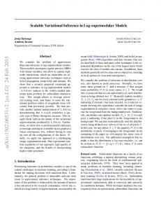
Figure 1: An image from the Sloan Digital Sky Survey [1], showing a galaxy from the constellation Serpens, 100 million light years from Earth, along with several other galaxies and many stars from our own galaxy.

We focus on modeling images of stars and galaxies—celestial bodies whose characteristics are effectively static during human lifetimes. The model we present here applies exclusively to stars; modeling galaxies and stars together is the focus of ongoing work.

2

The model

Celeste is a generative probabilistic model of astronomical images, represented graphically in Figure 2. In this section we describe how Celeste relates stars’ latent characteristics to the observed 1

pixel intensities in each image. The physics, and the instruments themselves, require us to account for a number of details. We explain in stages. 2.1 Stars Celeste is hierarchical, with stars atop pixels. We suppose images have been resampled to a common pixel grid. Let An denote the pixel grid for image n, with 20 pixels of padding on each border; any stars contributing photons to image n must have coordinates in An . For each star s = 1, . . . , S, the latent random 2-vector us encodes its position, in image-pixel coordinates. The prior distribution on the (us ), for image n, is jointly iid uniform: us ∼ Uniform (An ) .

star

S image lter band

PSF component

pixel

(1) M

Inference in Celeste is based on a known value of S; in Section 3.1 we describe our approach to setting that value.

K B N

The scalar parameter γs encodes a star’s observed Figure 2: The Celeste graphical model. brightness—the total radiation from the star that is ex- Shaded vertices represent observed random pected to pass through a unit area of the Earth’s sur- variables. Empty vertices represent latent face, facing the star, per unit time. The scalar param- random variables. Black dots represent eter τs encodes a star’s temperature in Kelvin. We constants. Edges signify conditional depentreat γs and τs as fixed parameters to estimate, rather dency. Rectangles are “plates”; they reprethan random variables, in order to improve the behav- sent independent replication. ior of our current variational optimization algorithm. Adding posterior uncertainty about γs and τs is a subject of research. 2.2 Radiation at different wavelengths In Celeste, the total rate of radiation arriving from a light source s, across all wavelengths, is proportional to its brightness γs . The distribution of that total rate across wavelengths depends on the nature of the light source. We model stars as idealized radiation sources, so-called “blackbodies”. The wavelength distribution for a blackbody of temperature τ is given by Planck’s law, a cornerstone of modern physics:  −1   2πc2 h hc I(τ, λ) = − 1 . (2) exp λ5 λkτ Here λ is a particular radiation wavelength, h is Planck’s constant, k is Boltzmann’s constant, and c is the speed of light. This simplification of the star source function could be replaced with a more realistic alternative if warranted, without complicating the inference. 2.3 Filter bands Cameras for optical astronomy typically use charge-coupled devices (CCDs), which convert light into electrons [5]. A CCD is a grid of millions of pixels. It is designed to sum the radiation arriving at a pixel across all the wavelengths in a designated interval, or “band”—its filter band. Most telescopes have several filters, enabling them to measure radiation in multiple bands. In the Celeste model, the number of measured bands is B. The CCD for filter-band b has a corresponding filter function ηb (λ). It indicates what fraction of arriving photons at wavelength λ the CCD will successfully detect, for each λ in band b. Thus, the final readout at each pixel is a weighted integral dλ of the in-band radiation arriving at that pixel, with weights ηb (λ). 2.4 Point-spread functions Astronomical images are blurred by a combination of small-angle scattering in the earth’s atmosphere, the diffraction limit of the telescope, optical distortions in the camera, and charge diffusion within the silicon of the CCD detectors. Together these effects are called the point spread function (PSF) of a given image. Stars (other than our Sun) appear intrinsically as point sources, but, because of the PSF, their photons are spread over typically dozens of adjacent pixels. We model the action of the PSF as a mixture of K Gaussians. Consider pixel m (in band b of image n), having coordinates 2

cm . The probability that a photon from star s, positioned at us in pixel coordinates, lands on m is obtained from the density K X
¯ nbk . fs (n, b, m) = α ¯ nbk φ cm ; us + ξ¯nbk , Σ (3) k=1

¯ nbk ) are the parameters of the Here φ is the bivariate normal density. Both K and the (¯ αnbk , ξ¯nbk , Σ PSF, determined a priori. 2.5 Sky noise The Earth’s atmosphere reflects terrestrial light, creating noise in each telescopic image. We model this noise as a homogeneous spatial Poisson process, independent of all light sources. The sky-noise process produces photons at rate nb uniformly, for each pixel in band b of image n. The noise rate depends on the image and the band because atmospheric conditions vary over time. Also, the atmospheric effects differ for imaging targets closer to the horizon. 2.6 The likelihood function We now put the preceding five subsections together to describe the distribution of pixel intensities, conditional on the locations of all light sources. For each band b, we know the values of the filter function ηb (λ) on a grid Υb of λ values—this is a matter of instrument design. If there were no PSF, the fraction of arriving photons detected at a band-b pixel containing a temperature-τ star would be Z 1 X Ib (τ ) = I(τ, λ) ηb (λ) dλ ≈ I(τ, λ)ηb (λ). (4) |Υb | λ∈Υb

When we further account for the PSF, the sky noise, and all stars, the total number of photons arriving at pixel m (in band b of image n) becomes xnbm |u, τ, γ ∼ Poisson (F (n, b, m)) . (5) Here the Poisson rate parameter F (n, b, m) is the superposition of all the relevant independent Poisson rates, with light-source photons passing through the PSF: S X F (n, b, m) = n + γs Ib (τs )fs (n, b, m). (6) s=1

3

Variational inference

Let u = (u1 , . . . , uS ) be the stars’ positions and let x = (x111 , . . . , xN BM ) be the pixel intensities. Computing the posterior p(u|x) is intractable: to apply Bayes’ rule exactly, we need to evaluate Z Y N Y B Y M S Y p(x) = p(xnbm |u) p(us ) du. (7) n=1 b=1 m=1

s=1

But the S-dimensional integral in (7) does not generally decompose into a product of lowdimensional integrals, and therefore cannot be computed. Instead, we find a distribution that approximates the posterior well. For any distribution q over u, log p(x) ≥ Eq [log p(x, u)] − Eq [log q(u)] =: L(q). (8) We call L the evidence lower bound (ELBO). To find a distribution q ? that approximates the true posterior well, we maximize the ELBO over a set of candidate q’s. To facilitate optimization, we restrict this set to distributions in which the (us ) are independent (the “mean field” assumption) and q(us ) ∼ Normal (Λs , Ξs ) . (9) ? Then finding q is equivalent to finding the optimal (Λs , Ξs ) for every star. By design, the expectations in L can all be evaluated analytically. Space constraints prevent us from showing the full derivation here. Key results include, for a particular image n, band b, and pixel m, S X
¯ nbk + Ξs Eq [F (n, b, m)] = n + γs Ib (τs )φ cm ; ξ¯nbk + Λs , Σ (10) s=1

and ( Eq [log F (n, b, m)] = log n +

S X K X

) exp (Eq [log ysk ]) ,

where

(11)

s=1 k=1


¯ nbk . ysk = γs Ib (τs )¯ αbnk φ cm ; us + ξ¯nbk , Σ 3

(12)

3.1

Optimization

To initialize our variational optimization, we convolve the images with matched filters to increase the signal-to-noise ratio [7]. We find each pixel whose value exceeds both the values of its neighboring pixels and an upper bound on the number of photons that could come from sky noise. We initialize the center of each such pixel as a light source. The number of such pixels determines S, the number of light sources we will assume are present in the image. In future work we will perform posterior inference about S as well. Next, we minimize L from equation (8) with L-BFGS [8] and automatic differentiation [9]. Because L is not globally convex, the optimization path matters. For a particular filter band b0 , we reparameterize L using γs0 := γs Ib0 (τs ). We run L-BFGS several times, optimizing different blocks of coordinates. First, we optimize the (γs0 ) simultaneously for all stars, with the remaining parameters fixed, using just the pixels from band b0 . For this band, because Ib0 (τs ) appears in both the numerator and the denominator, L is constant with respect to the (τs ). In other words, we do not need an estimate of the (τs ) to estimate the (γs0 ) from this band. Next, we optimize the (τs ) with L-BFGS for all stars and images simultaneously, with the other parameters fixed. Finally, we simultaneously optimize all parameters over all stars and images.

4

Experiments

We validated our procedure on synthetic data. To generate images, we set the (τs ) and (us ) to the temperatures and locations of actual stars and used the point spread functions from actual images, as approximated by a mixture of K = 3 Gaussians. For N = 1 image and B = 3 filter bands, we drew pixel values xnbm from (5). On synthetic data, our procedure converged consistently and quickly, for a wide range of iniFigure 3: Left is a 51 pixel × 51 pixel sub-region tial estimates of the variational parameters and of an astronomical image, captured through the the unknown constants. Moreover, it recovered r band filter. Each pixel’s value corresponds to the true locations and temperatures: the average the number of photons that hit it. The right panel distance of the posterior mean star locations Λs shows Eq? [F (n, b, m)], the mean of xnbm with from the truth—approximately 0.40 pixels upon respect to our posterior approximation. initialization—decreased to 0.01 pixels. For simulated stars with temperatures ranging from 4000◦ K to 9000◦ K, the average discrepancy of estimated temperature was 55◦ K. We also applied our procedure to a collection of 61 images from telescopes, each captured through five different filter bands, containing a total of 113 stars and approximately 150,000 pixels. These images do not overlap. We are planning an analysis of a data set five orders of magnitude larger, whose images have little overlap. These images will be processed largely in parallel, on a supercomputer, with minimal communication overhead. Plots like Figure 3 reveal that the approximate posterior predictive means of xnbm match the observed data. Our approximation of the point spread function is accurate, and our initialization routine has found the right number of stars. Though the true locations of the stars in the images are unknown, we validate our procedure by comparing our estimates to those from existing star catalogs. At initialization, the star locations Λs differed from the existing star catalogs by 0.40 pixels on average. After optimization, they differed by 0.22 pixels on average. (This ≈50% error reduction is significant to astronomers.) Thus, the variational inference improves on the initialization method. Nine stars in our dataset have been observed with a spectrograph. From the resulting spectra, we estimated the temperature of each star from its peak wavelength. These estimates—though not highly accurate—are independent of the estimates from the Celeste model. According to the spectra, the star temperatures range from 3200◦ –7500◦ K. The median and mean differences between the spectral estimates and Celeste’s estimates are 435◦ K and 735◦ K, respectively. These differences are larger than Celeste’s misfit on synthetic data: our modeling assumptions are inexact on real data, and ground truth was only available for the synthetic data. Still, Celeste’s temperature predictions agree closely with the independent spectral estimates: a no-intercept regression of them on Celeste’s predictions has slope 0.95. The F -test for addition of that slope to an intercept has p-value 0.0024. 4

Acknowledgments This work was supported by the Director, Office of Science, Office of Advanced Scientific Computing Research, Applied Mathematics program of the U.S. Department of Energy under Contract No. DE-AC02-05CH11231. We thank the anonymous referees for their helpful comments.

References [1] Sky images observed by the SDSS telescope. http://classic.sdss.org/gallery/ gal_data.html, 2014. [Online; accessed October 9, 2014]. [2] R. H. Lupton, Z. Ivezic, et al. SDSS image processing II: The photo pipelines. Technical report, 2005. [3] C. Stoughton, R. H. Lupton, M. Bernardi, et al. Sloan Digital Sky Survey: Early Data Release. The Astronomical Journal, January 2002. [4] L. Miller, T. D. Kitching, et al. Bayesian galaxy shape measurement for weak lensing surveys I. Methodology and a fast-fitting algorithm. Monthly Notices of the Royal Astronomical Society, 2007. [5] The dark energy survey. http://www.darkenergysurvey.org/, 2014. [Online; accessed October 9, 2014]. [6] Large synoptic survey telescope. http://www.lsst.org/lsst/about, 2014. [Online; accessed October 7, 2014]. [7] D. O. North. An analysis of the factors which determine signal/noise discrimination in pulsedcarrier systems. Proceedings of the IEEE, 1963. [8] D. C. Liu and J. Nocedal. On the limited memory BFGS method for large scale optimization. Mathematical programming, 1989. [9] J. Rauch et al. ForwardDiff.jl: Julia package for performing forward mode automatic differentiation. https://github.com/JuliaDiff/ForwardDiff.jl, 2014.

5