Change-point Estimation via Empirical Likelihood ... - Semantic Scholar

Change-point Estimation via Empirical Likelihood for a Segmented Linear Regression Zhihua Liu and Lianfen Qian

∗

Department of Mathematical Science, Florida Atlantic University, Boca Raton, FL 33431, USA Abstract For a segmented regression system with an unknown change-point over two domains of a predictor, a new empirical likelihood ratio statistic is proposed to test the null hypothesis of no change. Under the null hypothesis of no change, the proposed test statistic is empirically shown asymptotically Gumbel distributed with robust location and scale parameters against various parameter settings and error distributions. Under the alternative hypothesis with a change-point, the test statistic is utilized to estimate the change point between the two domains. The power analysis shows that the proposed test is tractable. An empirical example on analyzing the plasma osmolality data is given.

Keywords: Empirical likelihood ratio, Gumbel extreme value distribution, segmented linear regression, change-point.

1

Introduction

In the classical regression setting, the regression model is usually assumed to be of a single parametric form on the whole domain of predictors. However, a piecewise regression model ∗

Corresponding author. Email: [email protected]

1

is used to show that the parameters of the model can be different on different domains of the predictors. In the last thirty years, a considerable body of techniques have been developed for hypothesis testing, parameter estimation and related computing program on detecting change points for piecewise regression models. One special and commonly used piecewise regression model is the two-phase linear regression model. The regression function of this model is a piecewise linear function. One can define this more precisely as follows. Let Y be the response variable and X be a univariate predictor so that (X, Y ) is a bivariate random vector with E|Y | < ∞. Suppose that {(Xi , Yi )}ni=1 is a sequence of independent observations of (X, Y ) satisfying the following model: Yi = (α0 + α1 Xi )I(Xi ≤ τ ) + (β0 + β1 Xi )I(Xi > τ ) + ei

(1)

where {ei }ni=1 are independent error terms with mean zero. Let {X(i) }ni=1 be the order statistics of {Xi }ni=1 . If there is an unknown time k ∗ such that X(k∗ ) ≤ τ < X(k∗ +1) , then we shall call k ∗ the time of the change and τ the change point. Wide applications of two-phase linear regression models have appeared in diverse research areas. For example in environmental sciences, Piegorsch and Bailer [20] in their section 2.2 illustrate the usefulness of two-phase linear regression models with a series of examples. Lund and Reeves [14] utilize the model to detect undocumented change points. Qian and Ryu [24] fit the model with termite survival as Y and tree resin dosage as X. In the biological sciences, Vieth [31] applies the model to determine the osmotic threshold by fitting arginine vasopressin (AVP) concentration against plasma osmolality in plasma of conscious dogs. In medical science, Smith and Cook [28] use piecewise linear regression model to fit some renal transplant data. Other applications can be found in epidemiology (Ulm [30], Pastor and Guallar [19]), software engineering (Qian and Yao [22]), econometrics (Chow [3], Koul and Qian [13], Fiteni [8], Zeileis [32]) and so on. Hawkins [10] classifies the two-phase linear regression model (1) into two types of models: the continuous and the discontinuous. By continuous, it means that the regression function is

2

continuous at the change point τ ; that is, the change point τ satisfies the following equation: α0 + α1 τ = β0 + β1 τ.

(2)

If equation (2) is not satisfied, the model is discontinuous. The continuous model is also called the segmented linear regression model (Feder [6, 7]). Before applying the model (1), it is usual to test for the existence of a change point. There are two existing types of likelihood based approaches: The Schwartz Information Criteria (SIC) method (Chen [2]) and the classical parametric likelihood approach (Quandt [25, 26]). The SIC method, proposed by Schwartz [27], is a model selection criteria, defined as ˆ + k log n, SIC = −2 log L(θ) ˆ is the maximum where θˆ is the maximum likelihood estimator of the parameter vector, L(θ) likelihood function, k is the number of free parameters in the model, and n is the sample size. Chen [2] changes the task of hypothesis testing into model selection process by applying SIC method. See more details in Section 3. The classical parametric likelihood approach was first proposed by Quandt [25, 26] to detect the presence of a change point in a simple linear regression model. Quandt assumes that the error terms {ei }ni=1 are normally and independently distributed with mean zero and standard deviations σ1 if i ≤ k ∗ and σ2 if i > k ∗ . The likelihood ratio test statistic is Λ = max {λ(k)}, with λ(k) = −2 log 3≤k≤n−3

³σ ˆ k (k)ˆ σ n−k (k) ´ 1

2

σ ˆn

,

where σ ˆ is the estimator of the standard deviation of the errors for simple linear regression based on all observations; σ ˆ1 (k) and σ ˆ2 (k) are the estimators of σ1 and σ2 for fixed k, respectively. Large values of Λ suggest the existence of a change point. Quandt [25] conjectures that the asymptotic distribution of λ(k) is χ24 under the null hypothesis of no change (H0 ) for all k between 2 and n − 2. Under H0 assuming σ1 = σ2 for the segmented (continuous two-phase) linear regression model, Hinkley [11] and [12] claim that the asymptotic distribution of Λ is χ21 and χ23 , respectively. Feder [6, 7] comments that the distribution of Λ is not asymptotically χ2 . However, Feder indicates that there is 3

evidence for the existence of a limiting distribution of the likelihood ratio. Lund and Leeves [14] point out that the components of {λ(k)} are not independent. In fact, λ(k) and λ(k − 1) are correlated for a fixed k. This correlation makes the proof of the asymptotic distribution difficult. Lund and Leeves conjecture that the asymptotic distribution of Λ is related to the Gumbel extreme value distribution. In this paper, we address the afore-mentioned asymptotic distribution problem using a recently developed nonparametric empirical likelihood approach. Empirical likelihood (EL) as a nonparametric data-driven technique is first proposed by Owen [17]. EL employs the likelihood function without specifically assuming the distribution of the data. It incorporates the side information, through constraints or prior distribution, which maximizes the efficiency of the method (Owen [18]). First, we propose an EL based test statistic for testing the null hypothesis of no change. Through simulation studies, we have confirmed, under null hypothesis, that Lund and Leeves’s conjecture is correct for the empirical likelihood based method, though the original conjecture is for classical likelihood method, which is not solved yet. Then, if the null hypothesis is rejected, we construct an EL based estimator of the change point for the model (1) under the continuity constraint (2). The rest of the paper is organized as follows. Section 2 proposes the empirical likelihood ratio test statistic for the segmented linear regression model and defines the estimator of the time of the change if it exists. Section 3 shows empirically that the limiting null distribution of the proposed test statistic is the Gumbel extreme value distribution. It observed that the location and scale parameters of this asymptotic distribution were insensitive to the different settings of parameter vector and changes in the error distribution. The critical values for various significance levels, the size and the power performance of the test are reported. Furthermore, a comparison between the proposed EL based method and Chen’s [2] Schwartz information criteria (SIC) method is conducted. Section 4 presents an empirical example on analyzing the plasma osmolality data using the proposed ELR method.

4

2

EL Ratio Test and its Computing Algorithm

Assuming a known change point, Dong [5] derives an empirical likelihood type Wald (ELw) statistic to test the equality of two coefficient vectors from two linear regression models. To be more precise, let α ˆ and βˆ be the least squares estimators of the regression coefficient vectors, respectively. Under the normality assumption of the errors, Dong’s ELw test statistic has the form ˆ 0 [˜ ˆ ELw = (ˆ α − β) σ12 (X01 X1 )−1 + σ ˜22 (X02 X2 )−1 ]−1 (ˆ α − β) where Xi is the design matrix and σ ˜i2 is the EL estimator of σi2 , the variance of the errors, for the ith regression model (i = 1, 2). Dong concludes that the ELw test is asymptotically χ2p distributed under the null hypothesis H0 : α = β ∈ Rp . Instead of assuming a known change point, we first derive an empirical likelihood based test statistic for testing the null hypothesis of no change. If a change point does exist, we construct the EL based estimator for the time of the change (k ∗ ), and hence for the change point τ . Unlike the method used by Dong, we neither require the assumption of normality on the errors nor do we need the time of the change between the two phases to be known. However, we do require that the two phases be continuous at τ ∈ [X(k∗ ) , X(k∗ +1) ). We address the following two important research issues for model (1) with continuity constraint (2): • To test simple linear regression versus two-phase linear regression with one single unknown change point. • To estimate the time of the change if it exists. Let α = (α0 , α1 )> and β = (β0 , β1 )> in model (1). Then the test of no change is equivalent to the test H0 : α = β. Throughout the rest of the paper, we assume that {Xi }ni=1 are already ordered. For a fixed k, we can separate the data into two groups: {(Xi , Yi )}ki=1 and {(Xi , Yi )}ni=k+1 . For each group, we apply simple linear regression to fit the data points by using the ordinary least squares (OLS) method. Let α ˆ (k) = (ˆ α0 (k), α ˆ 1 (k))> be the ˆ = (βˆ0 (k), βˆ1 (k))> be the OLS OLS estimator of α computed from {(Xi , Yi )}ki=1 and β(k)

5

estimator of β computed from {(Xi , Yi )}ni=k+1 . Then, the estimated errors are   Yi − [ˆ α0 (k) + α ˆ 1 (k)Xi ], i = 1, . . . , k; eˆi (k) =  Y − [βˆ (k) + βˆ (k)X ], i = k + 1, . . . , n. i 0 1 i Under the null hypothesis H0 : α = β, α ˆ 0 (k) and βˆ0 (k) should be close to each other, and similarly for α ˆ 1 (k) and βˆ1 (k). Therefore, we propose to switch the rules of the estimated regression coefficient vectors in estimating the errors for these two phases. That is, the estimated errors under H0 can be represented as follows:   Yi − [βˆ0 (k) + βˆ1 (k)Xi ], i = 1, . . . , k; e˜i (k) =  Y − [ˆ α (k) + α ˆ (k)X ], i = k + 1, . . . , n. i

0

1

(3)

i

Notice that under H0 , E[˜ ei (k)] = 0 for all k. Following Owen (1991), when a change does occur, we should reject H0 if the empirical likelihood ratio (ELR) R(k) = sup

n nY

n n ¯X o X ¯ nwi ¯ wi e˜i (k) = 0, wi ≥ 0, wi = 1

i=1

i=1

(4)

i=1

is small. The corresponding logarithm of ELR is −2 log R(k) = −2 sup

n nX

n X

log(nwi )|

i=1

wi e˜i (k) = 0, wi ≥ 0,

i=1

n X

o wi = 1 .

(5)

i=1

By the Lagrange multiplier method, we write G=

n X

log(nwi ) − nλ

n X

i=1

wi e˜i (k) − γ

i=1

à n X

! wi − 1 ,

i=1

where λ and γ are Lagrange multipliers. Take the derivative of G with respect to wi , set it equal to zero and solve to obtain wi (k) =

1 . n[1 + λ˜ ei (k)]

It follows that −2 log R(k, λ) = 2

n nX

o log [1 + λ˜ ei (k)] .

i=1

Define the score function n

−2∂ log R(k, λ) X e˜i (k) = . φ(k, λ) = 2∂λ 1 + λ˜ ei (k) i=1 6

(6)

Then, we have the profile logarithm of ELR for a fixed k: ˆ ˆ −2 log R(k) = −2 log R(k, λ), ˆ is determined by φ(k, λ) ˆ = 0. where λ Notice that the true time of the change k ∗ is unidentifiable under the null hypothesis H0 . ˆ Large values of −2 log R(k) correspond to a two-tailed alternative hypothesis being true. Therefore, we propose the following test statistic: ˆ Mn = max {−2 log R(k)}. 3≤k≤n−3

(7)

ˆ When −2 log R(k) is small for each possible k, Mn will be small, as is the case under the null ˆ ∗ ) and Mn should be statistically large, hypothesis. If a change occurs at k ∗ , then −2 log R(k ˆ thus we reject H0 . Notice that −2 log R(k) is an asymptotic χ21 statistic for each fixed k and n−3 ˆ the components of {−2 log R(k)} k=3 are not independent. In this paper, we show, through p simulation study, that the limiting null distribution of Zn = Mn is Gumbel extreme value

distribution which is similar to the parametric likelihood ratio result, see Cs¨org˝o and Horv´ath [4]. If the null hypothesis is rejected, we need to estimate the change point by maximizing ˆ ˆ −2 log R(k). Simulation studies show that −2 log R(k) is sensitive to outliers when k is too small or too close to the sample size n. This phenomena exists for the parametric likelihood ratio approach. In order to overcome this situation, we adopt the “trimmed” test statistic defined below: ˆ Mn0 = max {−2 log R(k)}, L≤k≤U

(8)

where the choice of L and U are arbitrary. Anything ranges from [ln n] to n1/2 has been used in the literature for the parametric likelihood ratio approach. For empirical likelihood method, we have tested various trimmed portion. For the sample sizes used in the simulation, too small tail portions do not work well. Hence in this paper, we choose L = [ln n]2 and U = n − L, where [x] means the smallest integer larger than x. Thus the empirical likelihood estimator of k ∗ is defined by ˆ kˆ∗ = min {k : Mn0 = −2 log R(k)} 7

(9)

and hence the empirical likelihood estimator of τ is defined as τˆ = Xkˆ∗ . To test whether H0 is true, we need to compute Mn . Without loss of generality, let the ordered predictor values be X1 ≤ X2 ≤ . . . ≤ Xn . The algorithm for computing Mn contains the following steps: 1. For a fixed k, k = 3, 4, . . . , n − 3, split the data into two groups referred to as the left-phase group {(Xi , Yi )}ki=1 , and the right-phase group {(Xi , Yi )}ni=k+1 . 2. For each k, fit the points into a linear model to obtain α ˆ 0 (k), α ˆ 1 (k) from the left-phase group and βˆ0 (k), βˆ1 (k) from the right-phase group. 3. Calculate e˜i (k) = Yi − [βˆ0 (k) + βˆ1 (k)Xi ] for i = 1, . . . , k and e˜i = yi − [ˆ α0 (k) + α ˆ 1 (k)Xi ] for i = k + 1, . . . , n. 4. Use {˜ ei (k)}ni=1 as the input in the el.test function in R package (emplik) to compute ˆ −2 log R(k). n−3 ˆ 5. For each possible k, repeat step 1 to 4 to obtain a sequence of {−2 log R(k)} k=3 . The p maximum of this sequence is Mn . If Zn = Mn is larger than the critical value Gα

where P (Zn ≥ Gα ) ≤ α, H0 is rejected. So the corresponding minimum argument of Mn0 , kˆ∗ , is the EL estimator of k ∗ if we reject the null hypothesis of no change. Remark: We note that the mean response in a segmented regression model is a single linear piece under the null hypothesis. Hence, step 3 utilizes the single linear piece property to calculate the residuals. While step 4 combines the residuals from step 3 and sets the expected value of the overall residuals equal to zero through el.test.

3

Empirical Distribution of Zn

The algorithm presented above enables us to conduct simulation studies to show that the empirical distribution of Zn under the null hypothesis is the Gumbel extreme value distribution,

8

a subfamily of the Generalized Extreme Value (GEV) distribution. The GEV distribution has the following cumulative distribution function: n F (x; µ, σ, ζ) = exp

h ³ x − µ ´i−1/ζ o − 1+ζ , for x ∈ R and 1 + ζ(x − µ)/σ > 0, σ

where µ ∈ R is the location parameter, σ > 0 is the scale parameter and ζ ∈ R is the shape parameter. The shape parameter ζ dominates the tail behavior of the distribution. When ζ → 0, the limiting distribution of the GEV distribution is the Gumbel (G) extreme value distribution, given by n FG (x; µ, σ) = exp

− exp

h −(x − µ) io σ

.

(10)

For a Gumbel extreme value distribution, the mean and the variance are µ + σa and σ 2 π 2 /6, respectively, where a is the Euler-Mascheroni constant 0.57721.... We use the fgev function in R package (evd) to estimate the location µ, the scale σ and the critical values of FG . The function fgev uses the maximum-likelihood fitting of the GEV distribution to estimate µ, σ and ζ. We can obtain estimates of µ and σ for the Gumbel extreme value distribution, by setting ζ = 0. Four simulation studies are reported in this section. We simulate 1000 samples with the sample values of the random predictor X generated from N (0, 1). The sample size n ranges from 30 to 500. Simulation I is to test the robustness of the proposed EL based test statistic and computes the critical values of Zn for the most popular nominal levels 0.10, 0.05 and 0.01, under the null hypothesis of no change. Data are generated from the simple linear regression Yi = γ0 + γ1 Xi + ei , i = 1, ..., n

(11)

with γ = (γ0 , γ1 )> = (1, 1)> and three types of error terms are considered: (i) Normal errors: {ei }ni=1 ∼ N (0, 0.12 ); (ii) Log-normal errors (heavy-tailed): {ei }ni=1 ∼ log N (0, 0.12 ) and (iii) [n/2]

Non-homogeneous errors: {ei }i=1 ∼ N (0, 0.12 ) and {ei }ni=[n/2]+1 ∼ N (0, 1.02 ). Table 1 shows that the estimated location and scale parameters of the asymptotic distribution increase as the sample size increases. More importantly, one observes that both the 9

Table 1: Robustness analysis for the estimated location and scale parameters, µ and σ respectively, of the limiting distribution of Zn under three types of error distributions. The type of error distribution (i) Normal

(ii) Log-normal

(iii) Non-homogeneous

n

µ

σ

µ

σ

µ

σ

30

8.511

2.453

8.531

2.624

8.299

3.181

50

12.169 3.338

12.212

3.277

11.554

3.981

100

18.625 4.535

18.424

4.464

17.674

5.744

500

46.000 9.105

46.950

9.301

44.985

10.064

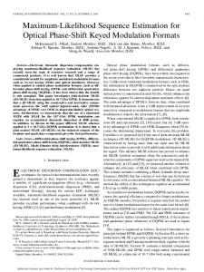
location and scale parameters are robust against changes to the distributions of the errors. This is consistent with the well-known property of the empirical likelihood method being of a nonparametric nature. The histograms and Q-Q plots of Zn for the 1000 replicates are shown in Figures 2-4 corresponding to three types of error distributions. The left panel shows the histograms of Zn where the solid line represents the estimated Gumbel density and the dashed line represents the estimated kernel density with Gaussian kernel using density function in R. The right panel shows the Q-Q plots of the Gumbel distributions. Simultaneously, the critical values of Zn with the nominal levels α = 0.10, 0.05 and 0.01 can also be derived by computing the quartiles of the simulated Gumbel extreme value distribution. The critical values of Zn are reported in Table 2. Simulation II was performed to show that the asymptotic distribution is robust against changes in the settings of parameter vector γ = (γ0 , γ1 )> in model (11). This simulation was carried out with five different settings of γ, a sample size of n = 100 and {ei }ni=1 ∼ N (0, 0.12 ). Table 3 indicates that the estimated location and scale parameters are robust to the settings of γ. Simulation III was carried out to compare the performance of the proposed EL based

10

Table 2: The critical values of Zn with α = 0.10, 0.05, and 0.01. The type of error distribution (i) Normal @

@

n

α @

0.10

0.05

(ii) Log-normal 0.01

0.10

0.05

0.01

(iii) Non-homogeneous 0.10

0.05

0.01

@ @

30

14.031 15.797

19.795

14.436 16.325

20.602

15.457 17.747

22.932

50

19.681 22.084

27.524

19.586 21.945

27.287

20.513 23.378

29.867

100

28.830 32.095

39.487

28.470 31.683

38.959

30.600 34.735

44.097

500

66.490 73.044

87.884

67.880 74.575

89.735

67.632 74.877

91.280

estimator and Chen’s SIC estimator of the true time of the change k ∗ . Chen’s SIC under H0 is SIC(n) = −2 log L0 (ˆ γ, σ ˆ 2 ) + 3 log n, where L0 (ˆ γ, σ ˆ 2 ) is the estimated maximum likelihood function under the null hypothesis of no change, γˆ is the estimator of γ and σ ˆ is the estimator of the standard deviation of the errors in model (11). For k ranging from 2 to n − 2, Chen’s SIC under H1 is SIC(k) = −2 log L1 (ˆ α0 (k), α ˆ 1 (k), βˆ0 (k), βˆ1 (k), σ ˆ 2 ) + 5 log n, where L1 (ˆ α0 (k), α ˆ 1 (k), βˆ0 (k), βˆ1 (k), σ ˆ 2 ) is the estimated maximum likelihood function under H1 . Therefore, the decision rule for selecting one of the n − 3 regression models is: select the model with no change if SIC(n) ≤ SIC(k) for all k; select a model with a change at kˆ∗ if SIC(kˆ∗ ) = min{SIC(k) : 2 ≤ k ≤ n − 2} < SIC(n).

Let ξ be the change in slope between the two phases for the segmented linear regression model (1) with the continuity constraint (2). We examine the effect of three different values of the change in slope on these errors settings: N (0, 0.52 ) and N (0, 0.12 ). The three different 11

Table 3: Robustness analysis of µ and σ with respect to γ when n = 100. γ > = (γ0 , γ1 ) (-1,1)

(2,-1)

(-3,-3)

(8,3)

(-3,5)

µ

18.625

18.824

18.629

18.500

18.931

σ

4.535

4.157

4.263

4.140

4.789

values of the change in slope are (a) small change of slopes with ξ = 0.5; (b) moderate change of slopes with ξ = 2; (c) large change of slopes with ξ = 4. When the X values are too close together, it is hard to detect the true time of the change. The acceptable deviation of kˆ∗ from k ∗ depends on the sample size and the range of the X values. In order to compare these two methods, we propose the following fine tuned acceptable deviation D:

¸ U −L , D= A ·

where A is the range of the X values, L = [ln n]2 and U = n − L are the fine tuning portion in the definition of the trimmed test statistic Mn0 . For X ∼ N (0, 1.02 ), we take A = 6. Then when n = 50, D = 3 with L = 16 and U = 34. For the purpose of illustration, we report the simulation results for the sample size n = 50 and k ∗ = 25 for the errors generated from N (0, 0.52 ) and N (0, 0.12 ). Let d = |kˆ∗ − k ∗ | be the absolute value of the bias between the true time of the change k ∗ and the estimate kˆ∗ , and RF be the relative frequency of the deviation d no more than the acceptable deviation D = 3. Table 4 reports the frequency distribution of d and the relative frequency of d ≤ 3. The simulation result indicates that the proposed method works slightly better than the SIC method to capture the true time of the change (d = 0). The relative frequency of both methods increases as the standard deviation (σ) of the errors decreases. When σ = 0.5 (the ratio of signal to noise is 2), both methods are not working well, though the proposed method works much better than SIC method for small to moderate change of slopes. When σ = 0.1 (the ratio of signal to noise is 10), these two methods are comparable. One also notices that 12

Table 4: The frequency distribution of d = |kˆ∗ − k ∗ | and the relative frequency RF = # of {d ≤ 3} % for ELR and SIC methods, when sample size n = 50 and the true time of 10 the change k ∗ = 25. N (0, 0.52 ) ξ = 0.5

ξ=2

N (0, 0.12 ) ξ=4

ξ = 0.5

ξ=2

ξ=4

d

ELR

SIC

ELR

SIC

ELR

SIC

ELR

SIC

ELR

SIC

ELR

SIC

0

26

14

57

51

91

81

172

169

193

189

301

299

1

40

28

155

90

170

165

298

269

317

301

316

317

2

46

24

118

99

203

198

167

189

198

217

187

196

3

55

29

102

128

165

172

101

116

119

128

71

68

4

41

30

84

113

103

128

81

79

78

89

64

55

5

85

26

82

94

98

103

86

85

54

59

34

32

6

74

17

79

88

89

64

79

69

30

11

12

24

≥7

633

832

323

337

81

89

16

24

11

6

15

9

RF (%)

16.7

9.5

43.2

36.8

62.9

61.6

73.8

74.3

82.7

83.5

87.5

88.0

as the change of slopes increases, the absolute value of the bias is getting smaller and the relative frequency is increasing. The simulation results for various sample sizes ranging from 30 to 500 show the similar pattern. From Table 4, one notices that the acceptable deviation also depends on the signal to noise ratio and change of slopes. The detection is easier for larger change of slopes than small to moderate, as does the signal to noise ratio.

Simulation IV is performed to study the size and the power performance of the proposed test for two types of error distributions. Table 5 shows the size and the power of the proposed test for a variety of sample sizes and true times of the change. The size is computed by using the estimated critical value of Gumbel distribution. We simulated 1000 samples from the model (11) with parameter vector γ = (1, 1)> , and the size is estimated by the proportion of

13

Table 5: The size and the power of Zn . The type of error distribution (i) Normal @

n

@

(ii) Log-normal

30

50

100

500

30

50

100

500

0%

0.045

0.049

0.050

0.050

0.054

0.054

0.048

0.050

20%

0.884

0.896

0.969

0.987

0.992

0.993

0.994

0.996

30%

0.897

0.897

0.968

0.987

0.997

0.995

0.995

0.994

40%

0.892

0.897

0.969

0.987

0.995

0.990

0.995

0.996

50%

0.908

0.898

0.960

0.987

0.996

0.982

0.995

0.996

k∗ n

@

@ @

samples resulting rejection of the null hypothesis falsely, which means test statistic is larger than the critical value. This study indicates that the proposed test statistic is able to control the size and attains a high power when the sample size is large.

4

Applications

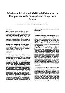
This section applies the proposed ELR method for the segmented linear regression to plasma osmolality data set. The data set was collected to show arginine vasopressin (AVP) concentration in plasma as a function of plasma osmolality in conscious dogs. Using parametric maximum likelihood method under normality assumption for errors, Vieth[31] utilizes the segmented linear model to fit arginine vasopressin (AVP) concentration against plasma osmolality in plasma of conscious dogs to determine the osmotic threshold. Our proposed ELR method does not require the normality assumption of the errors in nature. Figure 1(a) is the scatter plot, overlaid with the fitted segmented regression function, of the data with the estimated change point at τˆ = 302, corresponding to the osmotic threshold and indicated by the vertical dash line. We used the ELR method to plot −2 log ELR(k) for each possible time of the change between L and U; shown in Figure 1(b). The estimated

14

(b)

100

0

50

5

AVP(pg/ml)

−2logELR(k)

10

150

15

(a)

290

295

300

305

310

315

20

Plasma osmolality(mOsm/kg)

30

40

50

60

k

Figure 1: (a) the scatter plot of AVP versus plasma osmolality with fitted segmented linear regression. (b) The plot of −2 log ELR(k) versus all the possible time of the change k in [L, U]. time of the change is kˆ∗ = 42 highlighted by the solid dot. Then the estimated change point is τˆ = 302, and the least squares fitted segmented linear regression is AVP = −0.002+0.01∗plasma osmolality+0.52∗(plasma osmolality−302)+ , where (a)+ = max(0, a). The corresponding R2 is 73% with estimated standard deviation of 1.60.

5

Conclusion

This paper proposes a nonparametric empirical likelihood based test statistic for the detection of potential change points in segmented linear regression models. If the change point is identified, then an empirical likelihood based change point estimator is defined along with the estimator of the regression coefficients. Under the null hypothesis of no change, the simulation studies show that the proposed test statistic is asymptotically Gumbel extreme value distributed. The asymptotic distributions of the estimated location and scale parameters were shown to be robust under the different 15

settings of the parameter vector and the different types of error terms. The location and scale parameters are increasing functions of the sample size. Then, the simulation under the alternative hypothesis shows that the proposed test is able to control the size and attain a high power when the sample size is large. Finally, it is shown that the proposed empirical likelihood method performs better than SIC method in accurately detecting the true time of the change. However, allowing an acceptable deviation, the proposed method and Chen’s SIC method are comparable overall. An empirical example on analyzing the plasma osmolality data is given. The simulation and data analysis programs in R are available from the first author.

Acknowledgments:

The authors wish to thank the Editor and referees for their

valuable comments and suggestions that helped to improve the presentation of the paper.

References [1] Berman, N.G., et.al. (1996). Applications of segmented regression models for biomedical studies. American Journal of Physiology , 270, 723-732. [2] Chen, J. (1998). Testing for a change point in linear regression models. Communications in Statistics-Theory and Methods, 27:10, 2481-2493. [3] Chow, G. (1960). Tests of equality between two sets of coefficients in two linear regressions. Econometrica, 28, 591-605. [4] Cs¨org˝o, M. and Horv´ath, L. (1997). Limit theorems in change-point analysis, Wiley Series in Probability and Statistics. [5] Dong, L.B. (2004). Testing for structural change in regression: an empirical likelihood approach, Econometrics Working Paper, 0405. [6] Feder, P.I. (1975a). Asymptotic distribution theory in segmented regression problemsidentified case. The Annals of Statistics, 3, 49-83. 16

[7] Feder, P.I. (1975b). The log likelihood ratio in segmented regimes. The Annals of Statistics, 3, 84-97. [8] Fiteni, I. (2004). τ -estimators of regression models with structural change of unknown location. Journal of Econometrics, 119, 19-44. [9] Gbur,E.E., Thomas,G.L. and Miller,F.R. (1979). The use of segmented regression models in the determination of the base temperature in heat accumulation models. Agronomy Journal , 71, 949-953. [10] Hawkins, D.M. (1980). A Note on Continuous and Discontinuous Segmented Regressions, Technometrics, 22, 443-444. [11] Hinkley, D.V. (1969). Inference about the Intersection in Two-Phase Regression. Biometrika, 56, 495-504. [12] Hinkley, D.V. (1971). Inference in two-phase regression.Journal of the American Statistical Association, 66, 736-743. [13] Koul, L.H. and Qian, L.F. (2002). Asymptotics of maximum likelihood estimator in a two-phase linear regression model. Journal of Statistical Planning and Inference, 108, 99-119. [14] Lund, R. and Reeves, J.(2002). Detection of undocumented change points: A revision of the two-phase regression model. Journal of Climate, 15, 2547-2554. [15] Luwel K., Beem A.L., Onghena P. and Verschaffel L. (2001). Using segmented linear regression models with unknown change points to analyze strategy shifts in cognitive tasks. Behavior Research Methods, Instruments, & Computers. 33, 470-478(9) [16] Muggeo, V.M.R. (2003). Estimating regression models with unknown break-points. Statistics in Medicine. 22, 3055-3071.

17

[17] Owen, A.B. (1991). Empirical likelihood for linear models. The Annals of Statistics, 19, 1725-1747. [18] Owen, A.B. (2001). Empirical Likelihood, Chapman & Hall/CRC. [19] Pastor, R. and Guallar, E. (1998). Use of two-segmented logistic Regression to estimate change-points in epidemiologic studies. American Journal of Epidemiology , 148, 63142. [20] Piegorsch, W. W. and Bailer, A. J. (1997). Statistics for environmental biology and toxicology. Chapman and Hall. [21] Piepho, H. P. and Ogutu, J.O. (2003). Inference for the break point in segmented regression with application to longitudinal data. Biometrical Journal , 45, 591-601. [22] Qian, L.F. (1998). On maximum likelihood estimation for a threshold autoregression. Journal of Statistical Planning and Inference, 75, 21-46. [23] Qian, L.F. and Yao, Q.C. (2002). Software project effort estimation using two-phase linear regression models. Proceeding of The 15th Annual Motorola Software Engineering Symposium (SES). [24] Qian, L.F. and Ryu, S.Y.(2006). Estimating tree resin dose effect on termites. Environmentrics, 17, 183-197. [25] Quandt, R.E. (1958). The estimation of the parameters of a linear regression system obeying two separate regimes. Journal of the American Statistical Association, 53, 873880. [26] Quandt, R.E. (1960). Tests of the hypothesis that a linear regression system obeys two separate regimes. Journal of the American Statistical Association, 55, 324-330. [27] Schwartz, G. (1978). Estimating the dimension og a model. Annuals of Statistics, 6, 461-464. 18

[28] Smith,A.M.F. and Cook, D.G. (1980). Straight lines with a change point: A Bayesian analysis of some renal transplant data. Applied Statistics , 29, 180-189. [29] Toms, J.D. and Lesperance, M.L. (2003). Piecewise regression: A tool for identifying ecological thresholds. Ecology, 84, 2034-2041. [30] Ulm, K.W. (1991). A statistical method for assessing a threshold in epidemiological studies. Statistics in medicine, 10, 341-349. [31] Vieth, E. (1989). Fitting piecewise linear regression functions to biological responses. Journal of Applied Physiology, 67, 390-396. [32] Zeileis, A. (2006). Implementing a class of structural change tests: an econometric computing approach. Computational Statistics & Data Analysis , 50, 2987–3008.

19

Gumbel Q−Q plot

14 12 10

Sample Quantile

0.10

6

0.00

8

0.05

Density

0.15

16

(i) n=30

10

15

20

25

30

6

8

10

12

Zn

Theoretical Quantile

(i) n=50

Gumbel Q−Q plot

14

16 14 8

0.00

10

12

0.05

Density

Sample Quantile

0.10

18

20

22

0.15

5

20

30

40

10

12

14

16

18

Zn

Theoretical Quantile

(i) n=100

Gumbel Q−Q plot

20

22

25

Sample Quantile

20

0.06 0.04 0.00

15

0.02

Density

0.08

30

0.10

10

20

30

40

50

60

15

20

25

Zn

Theoretical Quantile

(i) n=500

Gumbel Q−Q plot

30

60

Sample Quantile

Density 0.02 0.00

40

0.01

50

0.03

0.04

70

0.05

10

20

40

60

80

100

120

140

35

40

45

50

55

60

65

70

Theoretical Quantile

Zn

Figure 2: The histograms and Q-Q plots of Zn under H0 with normal errors (i){ei }ni=1 ∼ N (0, 0.12 ) for four different sample size settings. The solid line represents the estimated Gumbel density and the dashed line represents the estimated kernel density. 20

Gumbel Q−Q plot

0.00

12 6

8

10

Sample Quantile

0.10 0.05

Density

0.15

14

16

0.20

(ii) n=30

10

15

20

25

30

6

8

10

12

Zn

Theoretical Quantile

(ii) n=50

Gumbel Q−Q plot

14

16 14

0.00

10

12

0.05

Density

0.10

Sample Quantile

18

0.15

20

5

5

10

15

20

25

10

30

12

14

16

18

Theoretical Quantile

Zn

(ii) n=100

20

0.00

15

0.02

0.04

Density

0.06

Sample Quantile

25

0.08

30

0.10

Gumbel Q−Q plot

20

30

40

50

14

60

16

18

20

22

Zn

Theoretical Quantile

(ii) n=500

Gumbel Q−Q plot

24

26

28

60 50

0.00

40

0.01

0.02

Density

0.03

Sample Quantile

0.04

70

0.05

10

20

40

60

80

100

120

40

140

45

50

55

60

65

70

Theoretical Quantile

Zn

Figure 3: The histograms and Q-Q plots of Zn under H0 with log-normal errors (ii) {ei }ni=1 ∼ log N (0, 0.12 ) for four different sample size settings. The solid line represents the estimated Gumbel density and the dashed line represents the estimated kernel density. 21

Gumbel Q−Q plot

12 10

Sample Quantile

0.10 0.00

6

8

0.05

Density

14

16

0.15

18

(iii) n=30

10

15

20

25

30

6

10 Theoretical Quantile

(iii) n=50

Gumbel Q−Q plot

14

14 12

0.06

0.08

Sample Quantile

16

0.10

18

0.12

20

12

8

0.00

0.02

10

0.04

Density

8

Zn

0.14

5

10

15

20

25

8

10

12

14

Zn

Theoretical Quantile

(iii) n=50

Gumbel Q−Q plot

16

18

0.00

15

20

Sample Quantile

0.04 0.02

Density

0.06

25

0.08

30

5

20

30

40

50

60

15

20

Zn

Theoretical Quantile

(iii) n=500

Gumbel Q−Q plot

25

60 50

Sample Quantile

0.02 0.00

40

0.01

Density

0.03

70

0.04

10

20

40

60

80

100

120

30

140

40

50

60

70

Theoretical Quantile

Zn

Figure 4: The histograms and Q-Q plots of Zn under H0 with non-homogeneous errors (iii) [n/2]

{ei }i=1 ∼ N (0, 0.12 ) and {ei }ni=[n/2]+1 ∼ N (0, 1.02 ) for four different sample size settings. The solid line represents the estimated Gumbel density and the dashed line represents the estimated kernel density. 22