Chemical Source Backtracking in Turbulent Boundary Layer (TBL) Ajith Gunatilaka1 , Alex Skvortsov1 , Branko Ristic2 , Mark Morelande3 , Dinesh Pitaliadda1 , Ralph Gailis1 1 DSTO,
HPPD, 506 Lorimer Street, Fishermans Bend, Vic 3207, Australia
2 DSTO,
ISRD, 506 Lorimer Street, Fishermans Bend, Vic 3207, Australia
3 University
of Melbourne, EEE Dept, Melbourne Systems Lab, , Vic 3052, Australia Email:
[email protected]
1
Introduction
The problem of chemical source backtracking is of great interest in application to ecological monitoring and defence systems. In the current paper we propose a framework to estimate the strength (emission rate) and the location of a chemical source which is continuously releasing a contaminant into the atmosphere. A network of spatially distributed chemical detectors is used to measure the concentration of contaminants at regular intervals and report to a fusion centre. Source parameters are estimated using a sequential Bayesian framework, with the posterior expectation approximated using Monte Carlo integration. A progressive correction approach is used to deal with problems caused due to the prior distribution being much more diffused compared to the likelihood. The statistical performance of the estimation algorithm is analysed using a synthetic dataset generated by using a well-known analytic solution of the turbulent diffusion equation for the mean concentration and a probability density function for the fluctuating part. The robustness of the estimation algorithm in the presence of imperfectly known environmental parameters is investigated by applying it to real experimental concentration data from the COANDA data set (2D laser-induced fluorescence measurements of concentration in a water channel), which mimicked atmospheric TBL flow over an urban canopy Yee et al. [2006].
2
Problem formulation
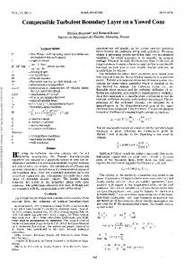
We consider the problem of backtracking a continuous point source of chemical agent based on concentration measurements acquired at a collection of chemical sensors placed at arbitrary but known positions. A graphical illustration of the problem is shown in Fig.1 in two-dimensions. We characterise the continuous point source by its location (x0 , y0 , z0 ) and its release (emission) rate Q0 (kg/s). However, throughout the paper we will assume that z0 = 0, hence the source parameter vector (which we need to estimate) can be written as: £ ¤T x = x0 y0 Q0 , (1)
Turbulent transport SOURCE
wind
SENSORS
Figure 1: Problem illustration in 2D where T denotes the matrix transpose. Let (xi , yi , zi ), i = 1, 2, . . . , S be the known position of the ith chemical sensor. Snapshots of concentration measurements from all sensors are acquired at discrete time steps and sent to a fusion centre for source estimation. In the sequential Bayesian framework, the goal is to estimate at each discrete-time step k, the posterior pdf p(x|z1:k ), where z1:k denote the cumulative set of all measurements available up to the kth time step. The posterior expectation will then be the the minimum mean square error (MMSE) estimator of the parameter vector x.
3 3.1
Turbulent diffusion and intermittency Modeling
We represent the concentration Ci that occurs at the ith sensor at a particular time instance as a sum of the mean and the fluctuating components: Ci = C¯i + C˜i .
(2)
For the model of mean concentration we use an analytic solution of the turbulent diffusion equation; the fluctuating part is modeled by a probability density function (pdf). We adopt a three-dimensional Cartesian coordinate system such that the x − y plane is the horizontal plane with the positive x axis equal to the wind direction, and the z axis pointing up. The mean wind velocity, assumed to be in the x direction, is expressed by µ ¶p z ux (z) = v0 , 0≤p≤1 (3) λ0 where v0 is the reference wind speed at a reference height λ0 . The mean concentration at a location (x, y, z) is expressed as C(x, y, z) = C y (x, y)C z (x, z),
(4)
with analytical expressions for C y and C z derived from the advection-diffusion equation of turbulent dispersion F.Pasquill and Smith [1983], A.Venkatram [2004], Huang [1999]. Details of the analytical model of mean concentration, have been omitted to save space but can be found elsewhere Skvortsov et al. [2007], Gunatilaka et al. [2008]. The fluctuating part of the concentration, C˜i in (2), is modeled by the probability density function of C with the mean, C, as a parameter (for details see Bisignanesi and Borgas [2007], Bisignanesi [2006], Borgas [2009]): µ ¶−γ ω 2 (γ − 1) ω C . (5) ρ(C|C) = (1 − ω)δ(C) + 1+ (γ − 2) C C (γ − 2) 190. 2
x = 190.5 1
0.8
0.6
0.6
0.4
0.4
0.2
0.2
¯ C ¯0 C
0.8
0 −6
−4
−2
0
2
y/ σy
4
6
Intermittency factor (w)
1
0
Figure 2: Variation of intermittency (Green circles) and normalised concentration (Blue squares) as functions of normalised y (cross-stream)-position Here the value γ = 23/6 was chosen to make it compliant with the theory of tracer dispersion in Kolmogorov turbulence Bisignanesi and Borgas [2007]. The parameter ω, which models the tracer intermittency in the turbulent flow, can be in the range [0, 1], with ω = 1 corresponding to the non-intermittent case. For w 6= 1, the pdf ρ of (5) has a delta impulse at zero, meaning that the measured concentration in the presence of intermittency can be zero on some occasions. Figure 2 shows plots of ω of COANDA water channel data (at downstream distance x = 190.5mm) and (C/C 0 ) as functions of normalised cross-stream position (y/σy ); C 0 is the value of C on the plume centreline and σy is the cross plume spread at this downstream distance. The value of ω is maximum on the plume centreline and it vanishes far from the centreline where C approaches zero. Figure 3(a) shows 1 − ω plotted in log scale against C/C 0 and Figure 3(b) shows ω and C/C 0 plotted in log-log scale.
0
0
10
10
−1
−1
10
ω
1−ω
10
−2
−2
10
10
−3
10
−3
0
0.1
0.2
0.3
0.4 0.5 ¯ C¯0 C/
0.6
0.7
0.8
0.9
10
−5
10
−4
10
−3
−2
10
10
−1
10
0
10
¯ C¯0 C/
(a)
(b)
Figure 3: Intermittency parameter ω of COANDA data plotted in: (a) exponential form (Eqn. 6) (b) power law form (Eqn. 7) Based on these results, we consider two models of intermittency: exponential model and power law model. A straight line in the first plot would suggest a model of the form
190. 3
Skvortsov et al. [2007]:
µ
¶ C 1 − ω ∼ exp −β , C0 while a straight line in the second plot would suggest a model of the form: µ ω = ωmax
C C0
(6)
¶ζ ,
(7)
where ωmax is the intermittency parameter on the centreline and ζ is a non-negative constant. In the limiting case of ζ = 0, ω is constant regardless of the distance to the point of interest from the centreline. If ζ = 1, (7) reduces to the linear model suggested in Borgas et al. [2008].
3.2
Implementation
To generate realistic concentration data, a synthetic environment was implemented in MATLABr . The mean concentration C at location (x, y, z) is a deterministic quantity and is computed directly using the analytic form discussed above. The measured concentration time series is generated by drawing random samples from the probability density function given in (5). The random number generator is implemented using the inverse transform method Robert and Casella [2004]. A uniform random number u ∼ [0, 1] is drawn and used to generate a random concentration value C using (8) where ω is the intermittency parameter and C is the mean concentration Gunatilaka et al. [2008]. i (¡ 1 ¢ h¡ 1−u ¢− γ−1 γ−2 C − 1 , u≥1−ω ω ω C= (8) 0, u < 1 − ω. The simulated mean concentration profile in the y − z plane due to a continuous point source located at the coordinate origin is shown in Figure 4(a). A concentration realisation across the same plane, generated assuming ω = 0.9, is shown in Figure 4(b). Corresponding mean and random concentration profiles along y direction at a fixed height are shown in Figure 5. Figure 6 shows a time series of the normalised concentration (C/C), generated at a single point within the plume.
4
Source parameter estimation
The Bayesian approach for parameter estimation assumes that a prior distribution π0 is available for the source parameters. In the case of chemical source backtracking problem, such prior distribution information may come, for example, from intelligence reports or observations of symptoms in personnel exposed to the chemical. Therefore, prior to receiving any measurements from the sensors, we assume that x ∼ π0 . The MMSE estimator, as the optimal Bayesian estimator, at time k is the posterior expectation: Z ˆ k = E(x|z1:k ) = xp(x|z1:k )dx, x (9)
190. 4
(a)
(b)
Figure 4: Simulated concentration data slices over y − z plane showing (a) the mean concentration C and (b) a random concentration realisation Concentration at x=10 and z= 0.15 16
25
Realisation Mean
14
20
10 15 C/C
Concentration
12
8
10
6 4
5
2 0 −2
−1.5
−1
−0.5
0 y
0.5
1
1.5
0 0
2
Figure 5: Simulated concentration profiles along y direction
500
1000 Time index (k)
1500
2000
Figure 6: A sample synthetic concentration time series
where1 p(x|z1:k ) ∝ π0 (x)
k Y
p(zm |x)
(10)
m=1
and p(zm |x) is the likelihood function of the measurement set at time m, zm = {z1m , . . . , zSm }, given x. According to Sec.3.1, this likelihood can be written as: S Y
S Y
ω 2 (γ − 1) p(zm |x) = p(zim |x) = [(1 − ω)δ(zim ) + ¯ C (γ − 2) i=1 i=1
µ
ω zim 1+ (γ − 2) C¯
¶−γ ](11)
The posterior pdf p(x|z1:k ) and, therefore, the posterior expectation cannot be found exactly for this problem. Monte Carlo methods have gained much interest for approximating integrals of the form of (9), because of their excellent performance and ease of implementation Robert and Casella [2004]. We use importance sampling, one such Monte Carlo technique, to approximate the posterior expectation. 1
Here we assume the temporal independence of concentration measurements, which is justified if the sampling interval is sufficiently long.
190. 5
In using importance sampling to approximate the integral of (9), the integral is approximated by the following weighted sum: ˆk ≈ x
N X
wkn xnk ,
(12)
n=1
xnk ,
where n = 1, 2, . . . , N is the nth sample drawn from an importance density q, and wkn is the corresponding importance weight computed as (13) wkn = C p(zk |xnk ), P n where C is a normalising constant chosen such that N n=1 wk = 1. Gunatilaka et al. [2008] However, because the prior will often be much more diffused than the likelihood (especially at the initial stages, for small k), straightforward use of the prior as the importance density will result in very few or even no samples being drawn from useful parts of the parameter space. A multistage approach referred to as progressive correction Musso et al. [2001] was used to estimate the source parameters Morelande et al. [2007], Gunatilaka et al. [2008].
5
Numerical Results
Results of Monte-Carlo runs of the progressive correction-based source estimation algorithm carried out on synthetic data using grids of different numbers of sensors, from Gunatilaka et al. [2008] are reproduced below to demonstrate how the root mean square position and source magnitude estimation errors vary as functions of sensor grid and measurement snapshots. More detailed results and discussion can be found in Gunatilaka et al. [2008]. 9x9 6x6 5x5 4x4 3x3
Source magnitude error (a.u.)
5.6
2
RMS position error (m)
9x9 6x6 5x5 4x4 3x3
5.7
10
10
1
10
10
5.5
10
5.4
10
5.3
10
5.2
10
5.1
10
1
2
3
4
5 6 7 Measurement number
8
9
10
(a)
1
2
3
4
5 6 7 Measurement number
8
9
10
(b)
Figure 7: RMS errors obtained by averaging over 100 Monte Carlo runs: (a) positional error; (b) emission rate error, versus discrete time Next we applied the progressive correction algorithm to data from the COANDA water channel experiment.The COANDA data set provides high resolution concentration data of a turbulent plume of fluorescent dye in a water channel, measured using laser-induced fluorescence measurement technique Yee et al. [2006]. Concentration measurements corresponding to plume cross sections at six downstream distances are available. 190. 6
At this early stage of our chemical source backtracking, we have made the simplifying assumption that the forward model for the mean concentration is perfectly known, and model parameters estimated through least squares fitting to COANDA data were used. While the best fitting parameters for data at individual downstream slices are slightly different, we used parameter values that best fit data at all downstream positions simultaneously. Obviously, assuming that the forward model is perfectly known overestimates the confidence on parameter estimates. We hope to remove the need for this assumption later by estimating the model parameters along with the source parameters. So far we have had only a limited amount of testing of our source backtracking algorithm using COANDA experimental data. Even when the correct forward model of the mean concentration is used, the source estimates were found to be quite sensitive to the intermittency model used. Figure 8 shows two examples of source backtracking results obtained by applying the progressive correction algorithm to COANDA data. Five sensors, equally spaced in cross-stream direction and located at equal height, were chosen along each of the six downstream distances where experimental concentration data were available. The pink dots in the figures denote these sensor locations and the size of the circles at these locations give a rough indication of the relative magnitude in a logarithmic scale of the instantaneous concentration measurements at the sensors. The green asterisk indicates the true source position. The cluster of red dots denotes the particles and the estimated source position is the centroid of these particle locations. The result in Figure 8(a) was obtained assuming the power law model of (7) with ζ = 0.45 and Figure 8(b) was obtained when ζ = 0 was used. In both cases wmax = 0.98 was assumed. Results were similar to Figure 8(b) when the exponential model of (6) was used. In the scenario shown here, the power law model with ζ = 0.45 appears to result in better source backtracking. Power law with ζ = 0 and the exponential model estimated the source position to be greatly upstream of the true position. Therefore, parameter ζ is important for developing an accurate backtracking model. 500 400 300 200
Y(m)
100 0 −100 −200 −300 −400 −500 −500
0
500
1000
0
500
1000
X(mm)
X(m)
(a)
(b)
Figure 8: Simulated concentration data slices over y − z plane showing (a) the mean concentration C and (b) a random concentration realisation
6
Conclusions
We described an analytical model for the mean concentration and a probabilistic model for the concentration fluctuations. A sequential Bayesian algorithm with progressive cor190. 7
rection for source parameter estimation was developed. This algorithm was tested using concentration data from a water channel experiment. The limited studies carried out so far demonstrates the potential of this algorithm for chemical source backtracking. But the sensitivity of the performance of the algorithm to model parameters including intermittency factors require further investigation. Estimating the model parameters along with the source parameters may be necessary to make the source backtracking algorithm more robust.
References A.Venkatram. The role of meteorological inputs in estimating dispersion from surface releases. Atmospheric Environment, 38(16):2439–2446, 2004. V. Bisignanesi. Scalar plumes in canopies and atmospheric surface layer. PhD thesis, School of Mathematical Sciences, Monash University, Australia, 2006. V. Bisignanesi and M. S. Borgas. Models for integrated pest management with chemicals in atmospheric surface layers. Ecological modelling, 201(1):2–10, 2007. M. Borgas. Multifractal coding for turbulent mixing of plumes. Submitted to New Journal of Physics, 2009. M. Borgas, R. Gailis, A. Skvortsov, and V. Bisignanesi. Simple models for surface-layer fluctuations. Submitted to Boundary Layer Meteorology, 2008. F.Pasquill and F. Smith. tmospheric Diffusion. John Wiley Sons, New York, 1983. A. Gunatilaka, B. Ristic, A. Skvortsov, and M. Morelande. Parameter estimation of a continuous chemical plume source. In Proc. 11th Int. Conf. on Information Fusion, Cologne, Germany, June 2008. C. Huang. On solutions of the diffusion-deposition equation for point sources in turbulent shear flow. Journal of Applied Metorology, 38:250–254, 1999. M. Morelande, B. Ristic, and A. Gunatilaka. Detection and parameter estimation of multiple radioactive sources. In Proc. 10th Int. Conf. Information Fusion, Qu´ebec, Canada, July 2007. C. Musso, N. Oudjane, and F. LeGland. Improving regularised particle filters. In A. Doucet, N. deFreitas, and N. J. Gordon, editors, Sequential Monte Carlo methods in Practice. Springer-Verlag, New York, 2001. C. P. Robert and G. Casella. Monte Carlo Statsitical Methods. Springer, second edition, 2004. A. T. Skvortsov, P. D. Dawson, M. D. Roberts, and R. M. Gailis. Modelling of flow and tracer dispersion over complex urban terrain in the atmospheric boundary layer. In Proc. 16th Australasian Fluid Mech. Conf., QLD, Australia, 2007. E. Yee, R. M. Gailis, A. Hill, T. Hilderman, and D. Kiel. Comparison of wind- tunnel and water-channel simulations of plume dispersion through a large array of obstacles with a scaled field experiment. Boundary-Layer Meteorol, 121:389–432, 2006. 190. 8