TURBULENT BOUNDARY LAYER ... - CiteSeerX

SHOCK/TURBULENT BOUNDARY LAYER INTERACTION ON A DOUBLE RAMP CONFIGURATION -EXPERIMENTS AND COMPUTATIONS U. Gaisbauer, H. Knauss, and S. Wagner Institut für Aerodynamik und Gasdynamik (IAG), Universität Stuttgart, Germany Y.V. Kharlamova, and N.N. Fedorova Institute of Theoretical and Applied Mechanics SB RAS, 630090 Novosibirsk, Russia Introduction In the last 50 years big efforts were done to get more understandings of the phenomenon of the shock boundary layer interaction in supersonic flow [1]. A lot of experiments with different purpose were carried out: 2D-cases with big and small ramp angles, swept and un-swept, 3D-cases with different geometries (ramps, flaps etc.). Also in the field of numerical computation there was a big success in simulating the above mentioned experiments ([2, 3] and others). In the past the main interest in the available literature, concerning the 2d, un-swept case, was focused on the single ramp with big ramp angles to achieve the desired compression. In the department of Aerospace Engineering at the Stuttgart University the “Special Research Center 259”, financed by the Deutsche Forschungsgemeinschaft (DFG), is established. The IAG is involved in this research program with its sub-project: Experimental Investigation of Compression Surfaces on the Forebody and Integrated Inlets of Air-breathing Hypersonic Vehicles. Here, the total incoming turbulent boundary-layer is not peeled off. In this content one of the main tasks was to create a highly integrated intake with low pressure drag. This requirement results in a double ramp configuration (shock/shock) with short length and moderate ramp angles. Under such conditions, the shock boundary layer interaction on both ramp inflections is coupled. Preceding measurements in a small suck down wind tunnel at R/m=10x106 and M=2.5 showed that for a fixed length of the first ramp of L=40 mm (L/δ ≈5) and an angle combination of 11° and 9°, required by another sub-project of the Special Research Center, no separation of the second shock took place [4]. From this point of view one important parameter for the separation of the second shock is the length of the first ramp normalized with the incoming boundary layer thickness just upstream of the first ramp kink: L/δ. In this content the question is to find the critical length of the first ramp to determine the beginning of separation of the second shock by varying the length with constant unit Reynoldsand Mach number for fixed ramp angles α1=11° and α2=9°. But first of all and of main interest for the whole shock/shock phenomenon is to specify the basic characteristics of the incoming boundary layer like thickness and state of the boundary layer. Parallel to this experiments, numerical simulation were made at ITAM by Y.V. Kharlamova and Dr. N.N. Fedorova with an RANS + k-ω turbulence model to predict the critical length of the first ramp. Experimental facility The experiments were carried out in the so called “shock wind tunnel”, SWK, of IAG, Stuttgart University. This short duration facilitiy is, according to the working principle, a kind  U. Gaisbauer, H. Knauss, S. Wagner, Y.V. Kharlamova, and N.N. Fedorova, 2002

56

of shock tube with a Laval nozzle. During one run there are two steady flow states of 2x120 ms. Because of the large test section (1.2×0.8 m2) investigations of models with large dimensions can be carried out from a Mach number range of M=1.75÷4.5 and a corresponding unit Reynolds number range of R/m=70×106÷30×106 [5]. Wind tunnel models and instrumentation At the beginning of all measurements and numerical simulations in the content of the shock/shock field, two basic problems appear: the determination of the basic flow on the flat plate and of the pressure distribution over the two ramps. To be able to receive measured data about this two main items, different models for different tasks were necessary. Consequently three flat plate models with different double ramp configurations were built. The basic model was always a flat plate with a sharp leading edge. The size was 0.6×0.2 m2. To reduce roughness due to the manufacturing the surface was polished. To simulate a real 2D flow over the flat plate, the model was completed with trapezoidal sidewings, designed with supersonic edges for M=2.54. The model was mounted on a special support to place the whole configuration outside the tunnel side wall boundary layer. Model 1: For the first investigations a model with static pressure tabs along the center line and in spanwise direction was manufactured. The static pressure distribution along the surface was determined with a fast responding pressure scanning system (PSI 8400-system with two scanner modules, 34 ports each) which allows 250 averages of the 64 pressure ports within the SWK runtime [6]. To measure and calculate the skin friction coefficient (cf), a Preston-tube was installed, bearing flat on the surface, adjustable along the center line [7]. Model 2: The second model was instrumented with three parallel to the center line shifted rows of McCroskey hot film sensors, driven in the CCA-mode with an overheat ratio of a = 0.6. Their spacing was ∆x = 15mm. The hot films were applicated on adjustable inserts, adapted to the plate surface by turning over in manufacturing to avoid artificial roughness [5]. This configuration was used to measure the development of the boundary layer and the location of transition. Additionally, the first double ramp model was installed at a position of x=450mm from the leading edge. The upper ramp was movable on the first to realize the variation of the distance between the two kinks. On the double ramp model the distance between the pressure ports was ∆x = 2.5 mm. Again the above mentioned PSI 8400-system with two pressure scanner modules came into operation. Model 3: The last used model was constructed modular to give the possibility of a variable sensor installation. Various sensors like different kind of hot films, the new developed Atomic Layer Thermo Pile (ALTP) [8] or an insert with static pressure ports were put in. A new 11°-ramp/plate insert was built with a spacing of ∆x = 1.25 mm between the pressure tabs. So it was possible to measure the static pressure distribution in front of the first kink and on the ramp simultineously with a very high resolution and without mechanical perturbation in the kink. The upper, 9°-ramp was unchanged. The position of the ramp configuration was at x = 420 mm due to constructive and gasdynamic requirements. The PSI 8400-system was again used. Additional an adjustable Pitot-probe with a resolution of ∆y = 0.04mm was installed to measure the boundary layer profile at a x-position of 380 mm normal to the plate surface. Data aquisition In all cases a 12bit A/D converter with a sampling rate of about 500kHz combined with a digital anti-aliasing filter was used. The monitoring and the data processing was made by programs written in LabVIEW at IAG.

57

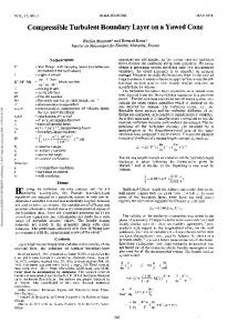
Numerical model The computations were performed on the basis of Favre-averaged Navier-Stokes equations closed by a two-equation k-ω turbulence model by Wilcox [9]. The computation domain is restricted by inlet and outlet sections choosen far enough from the interaction zone, solid surface on the bottom and free surface on the top boundary. No-slip condition for velocity and adiabatic condition for temperature are set on solid surfaces. So called "simple wave" conditions are used on the upper boundary. Profiles of all gasdynamic and turbulence parameters obtained using boundary layer approach are specified at the inlet section and "soft" conditions are used at the outlet section. A regular grid condensed to the rigid walls was used in calculations. Typically, the grid consists of 100÷200 nodes in y-direction and 200÷400 nodes in x-direction. About 50% of the grid nodes lay inside the boundary layer developed along the rigid wall. The four-step implicit finite-difference scheme of splitting according to the space directions realized by scalar sweeps was used for time approximation. TVD-type scheme based on Van Leer Vector Flux Splitting method [10] was used to construct the high resolution approximation of inviscid fluxes space derivatives. Viscous terms were differenced to the second order accuracy in a centered manner. The computational method is described in details in [11]. This original numerical algorithm has been used to compute various 2D turbulent supersonic separated flows and has shown a good potential to predict the properties of the investigated flows [12], [13]. Measurements and results In the present work the first main problem was to qualify the incoming flow field and the resulting boundary layer on the flat plate as a kind of basic flow, with great importance for the experiment and as well for the numerical computation. Therefore, at first the flow field on the flat plate without installed ramp was studied. Measurements of the static pressure with the above described model 1 were made. This results in a change of the normalized static pressure distribution along the center line (on a length of 330mm) of about 1.5%. In spanwise direction the influence of the kink in the leading edge, spreading in “Mach direction”, is also detectable but only with very small changes (~1÷1.5% of the mean static pressure). Other fluctuations could not be found, the conformity of the flow is within 1% [6]. As a first result the incoming flow can be qualified as two dimensional. In the next step measurements with a Preston-tube at different positions along the center line were done. From this Pitot-pressure distribution at R/m=12.7×106 results a transition Reynolds number of ReT=2×106 (Fig. 1), [7]. This could be verified with the hot film measurements of model 2. The investigation of the region with the maximum fluctuation level Urms/Umean (hot film output) leads also to ReT=2×106 (Fig. 2). With the Preston-tube data the skin friction coefficien cf was calculated for different positions, according to [14]. The result in the still transitional region (x=180mm) is a value of cf=3.1×10–3. In a more downstream position (x = 300mm) cf is reduced to 2.7×10–3 [7]. This trend is typical for the development of a supersonic boundary layer from the transitional to the fully turbulent state [15]. So it can be assumed that at the position of the first ramp kink (x=450mm) the boundary layer is turbulent, verified later. Parallel to the hot film measurements on model 2, the first ramp/ramp-configuration was installed. Measurements of the static pressure distribution on the flat plate and on the two ramps were made along the center line for R/m=12.7×106. The distance of the two ramp kinks was varied between L/δ=3.3÷7.4. In Fig. 3 the normalized pressure distribution for different distances of L/δ is plotted in the coordinate system of the flat plate. It seems that for L/δ=4.0 the second shock is still separated. For L/δ ≥ 5.0 the pressure plateau on the second ramp starts to 58

0.06

2.5E-03

p'/p(pitot) [/]

0.05 0.04

6

Re T * 10 1.99 1.7 1.7 1.7

hotfilm McCroskey flat plate SWK M=2.5

6

sensor position x pr

2.0E-03

x=156mm x=200mm x=225mm x=249mm

0.03

xpr [mm]

-6

1.5E-03

-6

ReT [10 ] R/m [10 ]

x = 156 x = 199 x = 229 x = 244

U´rms/Umean [/]

R/m * 10 12.7 8.5 7.4 6.8

1.99 1.79 1.58 1.68

12.7 9.0 6.9 6.9

1.0E-03

0.02

5.0E-04

0.01 0

0.0E+00 0

1

2

3 Re(x pr) [Mio]

4

0

Fig. 1. Normalised Pitot-pressure distribution.

1

2

3

-6

Re(pr) [10 ] 4

Fig. 2. Normalised hot-film output signal.

develop up to a constant value. But only a qualitative evaluation is possible, a further detection method was not used, e.g. to find a second inflection point for the separated case, like in [16]. A first comparison with the numerical simulation shows a different behaviour. In Fig. 4, for L/δ=4.1 no separation can be seen. In all the compared cases for L/δ the second shock is not separated. A big discrepancy appears between experiment and numeric. Obviously the used boundary layer thickness for normalization is different (see the label in Fig. 3 and Fig. 4). Up to this time there have been certain differences in the boundary conditions between experiment and numerical simulation: First, no exact measurement of the boundary layer at the ramp position was possible. As boundary conditions for the simulation only some other numerical computations were available [17]. Second, the experimental resolution in the pressure distribution, the spacing between the ports, was not high enough. Accordingly, the whole experiment and the numerical simulation must be improved by using a new wind tunnel model and by computing with the experimentally defined boundary conditions. As above described, model 3 gives the possibility to measure the static pressure with the desired higher resolution and to determine the boundary layer profile with the adjustable Pitotprobe. The position of the first ramp was at x = 420mm, to make sure to be in the fully turbulent region and not in the end of transition. The Pitot-pressure and the static pressure distribution were measured simultaneously. From the measured Pitot-pressure profile (Fig. 5) the boundary layer thickness was determined as δ = 5.0 mm by using the Pitot – Rayleigh-relation, according to the procedure described in [18], and by calculating the Mach number profile. The pure shape of the profile leads also to the conclusion that the boundary layer is turbulent [19]. It must be mentioned, that for each of the 54 data points one single run of the SWK was necessary. Therefore the unit Reynolds number with its fluctuations could be determined with an higher accuracy as before to R/m=12.63×106±0.17×106. Further on, under the assumption of a quasiadiabatic wall condition the velocity distribution was determined [20, 21]. Finally the

Fig. 3. Normalised static pressure distribution.

Fig.4. First computational results. 59

Fig. 5. Pitot pressure profile for the determination of the boundary layer thickness δ.

Fig. 6. Dimensionless velocity distribution according to V. Driest.

dimensionless velocity distribution u+(y+) could be calculated [22]. In fig. 6, u+(y+) and the loglaw with an assumed cf-value of 2.1×10–3 are plotted with a quite good aggrement between the measured and calculated data points in the lower region of the boundary layer. The turbulent character of the boundary layer is again evident and the above made assumtion can be verified. Consequently, as the first main results the incoming boundary layer on the flat plate in front of the first ramp kink can be qualified as turbulent and the boundary conditions for the future experiments and the numerical computations can be specified as: R/m=12.63×106±0.17×106, M∞=2.543±0.01, Me=2.51±0.02, cf =2.1×10–3, δ=5.0mm Parallel to the boundary layer investigations the static pressure distribution with the second ramp/ramp-model was measured. The variation of the distance L/δ started at L/δ=0, what means a single ramp situation with α1=20°, and went up to L/δ=8 in steps of ∆L/δ≈0.3. In Fig. 7 the normalized pressure distribution is plottet versus x/δ, in the cartesian plate coordinate system, where x/δ=0 indicates the position of the first kink. With an increased resolution compared to fig. 3, a clear development of the pressure distribution from the separated case to the fully developed pressure plateau on the first ramp is visible. Qualitatively, the latter case starts at L/δcritical=4 or 4.3. For smaller ratios of L/δ, one can assume that the two shock system is not totally developed and the second shock is still separated and moved upstream. A more detailed analysis of the experimental data are in a go and will be published later. In Fig. 8, for 5 different values of L/δ, the improved numerical results, computed with the measured boundary

Fig. 7. Development of the normalised static pressure distribution by varying L/δ; determined with improved model.

Fig. 8. Comparison of computed and measured static pressure distribution by using the exp. determined boundary conditions. 60

a) L/δ=3

b) L/δ=4

Fig. 9. Computed skin friction coefficient for different L/δ.

Fig. 10. Simulated Mach number distribution for different L/δ a) separated second shock b) wished two shock system.

conditions, are compared with the experiment. The agreement in the prediction of the pressure distribution is quite good, even in the inflection points due to the ramp/ramp-configuration. Beginning from a ratio of L/δ=4 the gradient in the normalized pressure distribution becomes smaller and at L/δ=5 the constant pressure plateau is detectable. This behaviour leads again to the conclusion that for values of L/δ