was then covered with rock wool and silver paper backed fiberglass for insulation. Fig. 3.7 shows ...... layer compared to the neutral profile, plus the reduction in vertical turbulence, as well as. 149 ...... Journal of Fluid Mechanics, 10:433,. 1961.
Density effects on turbulent boundary layer structure: from the atmosphere to hypersonic flow
Owen J.H. Williams
A Dissertation Presented to the Faculty of Princeton University in Candidacy for the Degree of Doctor of Philosophy
Recommended for Acceptance by the Department of Mechanical and Aerospace Engineering Advisor: Professor Alexander J. Smits
November 2014
© Copyright by Owen J.H. Williams, 2014. All rights reserved.
Abstract This dissertation examines the effects of density gradients on turbulent boundary layer statistics and structure using Particle Image Velocimetry (PIV). Two distinct cases were examined: the thermally stable atmospheric surface layer characteristic of nocturnal or polar conditions, and the hypersonic bounder layer characteristic of high speed aircraft and reentering spacecraft. Previous experimental studies examining the effects of stability on turbulent boundary layers identified two regimes, weak and strong stability, separated by a critical bulk stratification with a collapse of near-wall turbulence thought to be intrinsic to the strongly stable regime. To examine the characteristics of these two regimes, PIV measurements were obtained in conjunction with the mean temperature profile in a low Reynolds number facility over smooth and rough surfaces. The turbulent stresses were found to scale with the wall shear stress in the weakly stable regime prior relaminarization at a critical stratification. Changes in profile shape were shown to correlate with the local stratification profile, and as a result, the collapse of near-wall turbulence is not intrinsic to the strongly stable regime. The critical bulk stratification was found to be sensitive to surface roughness and potentially Reynolds number, and not constant as previously thought. Further investigations examined turbulent boundary layer structure and changes to the motions that contribute to turbulent production. To study the characteristics of a hypersonic turbulent boundary layer at Mach 8, significant improvements were required to the implementation and error characterization of PIV. Limited resolution or dynamic range effects were minimized and the effects of high shear on cross-correlation routines were examined. Significantly, an examination of particle dynamics, subject to fluid inertia,compressibility and non-continuum effects, revealed that particle frequency responses to turbulence can be up to an order of magnitude smaller than estimates made using a standard shock response test. The effect of over-large tripping devices was also found to increase the wake strength of the mean velocity profile as well iii
as freestream turbulence. A final assessment of the data reveals that Morkovin scaling collapses the streamwise turbulence profiles with DNS at the same Mach number. Wall-normal turbulence measurements remain compromised by limited particle frequency response.
iv
Acknowledgements I would like to begin by thanking by advisor, Lex Smits, for years of guidance and mentorship. His extreme level of support and patience has afforded me the freedom to work on the two turbulence problems I found the most interesting, even when the difficulty of the experiments and lack of sustained funding would have put a stop to such stubbornness under most other circumstances. He has taught me a great many skills that will serve me well, both academically and in the wider world. For all of this and much more, I am thankful. Much of the work presented in this thesis would not have been possible, or at least extremely delayed, without the countless hours of assistance received from Bob Bogart and Dan Hoffman. Bob’s experience and advice was instrumental to the construction of the thermally stratified wind tunnel during the first year of my PhD. Dan has worked tirelessly to maintain and improve the hypersonic wind tunnel and the compressors, valves, piping, and pressure tanks needed for its operation. While I have been able to provide a set of hands, much of the work required was previously way beyond my experience. Whether it was the rebuild of yet another compressor, strategizing the acquisition of a crane to fix the ejectors, replacement of almost every gasket and O-ring in the facility, jury rigging vacuum test equipment to test for leaks and calibrate the transducers or building/modifying test plates, Dan always had an idea how to make it happen or the experience to guide me. I do not think I will meet another person who will be able to say, “Ya, I think I have the parts for that” quite as readily. I would also like to thank my collaborators and lab mates for the conversations and experiences you have shared with me. Specifically, Dipatakar Sahoo for introducing me to PIV, and Tue Nguyen and Anne-Marie Schreyer, with whom I wrote my first paper. I am also thankful for the time spent with Peter Dewey, Anand Ashok and Leo Hellstr¨om, who began working with me in Lex’s lab at the same time, and have have been amazing friends and colleagues. v
I would also like to acknowledge my readers, Elie Bou-Zeid and Gigi Martinelli for their insightful comments and suggestions with regard to this thesis. Also my committee, Gigi Martinelli and Dick Miles for their guidance and support throughout my degree. Finally, I would like to thank my parents for all the guidance, patience and encouragement through all my years of education and growth. Without their support, I would not be where I am today. They always encouraged me to try new things and supported me through my movements from country to country in search of new and interesting opportunities. I cannot begin to express how much this has meant to me. I would also like to thank my girlfriend, Jodi, for putting up with me during this last year and for keeping me sane while being forced to relive the writing of her thesis all over again. I cannot thank her enough.
The thermally stable boundary layer research was supported by Princeton University’s Grand Challenges - Energy program and the Thomas and Stacey Siebel Foundation.
This dissertation carries the designation 3279T in the records of the Department of Mechanical and Aerospace Engineering.
vi
To my parents.
vii
Contents Abstract . . . . . . . . . . . . . . . . . . . . . . . . . . . . . . . . . . . . . . . . . .
iii
Acknowledgements . . . . . . . . . . . . . . . . . . . . . . . . . . . . . . . . . . . .
v
List of Tables . . . . . . . . . . . . . . . . . . . . . . . . . . . . . . . . . . . . . . .
xii
List of Figures . . . . . . . . . . . . . . . . . . . . . . . . . . . . . . . . . . . . . . . xiii 1
Introduction 1.1
1
Atmospheric and Hypersonic boundary layers: Why are they important? How do they differ? . . . . . . . . . . . . . . . . .
1.2
Difficulties obtaining accurate data / benefits of laboratory scale measurements . . . . . . . . . . . . . . . . . . . . . . . . . . . . . . . . . . . . . . . .
2
1
4
Background
6
2.1
Thermally Stable Boundary Layers . . . . . . . . . . . . . . . . . . . . . . .
6
2.1.1
Monin-Obukhov Similarity Theory (MOST) . . . . . . . . . . . . .
7
2.1.2
Other measures of stability . . . . . . . . . . . . . . . . . . . . . . . .
9
2.1.3
Stable boundary layer regimes . . . . . . . . . . . . . . . . . . . . . .
10
2.1.4
The critical Richardson number
. . . . . . . . . . . . . . . . . . . .
13
2.1.5
Previous experimental results . . . . . . . . . . . . . . . . . . . . . .
15
2.1.6
Challenges/Goals . . . . . . . . . . . . . . . . . . . . . . . . . . . . .
21
Hypersonic boundary layers . . . . . . . . . . . . . . . . . . . . . . . . . . .
21
2.2.1
22
2.2
van Driest scaling of the mean velocity . . . . . . . . . . . . . . . . viii
2.3 3
Morkovin’s hypothesis . . . . . . . . . . . . . . . . . . . . . . . . . .
25
2.2.3
Previous experimental results . . . . . . . . . . . . . . . . . . . . . .
28
2.2.4
Challenges/Goals . . . . . . . . . . . . . . . . . . . . . . . . . . . . .
33
Turbulent coherent structures
. . . . . . . . . . . . . . . . . . . . . . . . . .
40
3.1
PIV . . . . . . . . . . . . . . . . . . . . . . . . . . . . . . . . . . . . . . . . . .
41
3.1.1
Overview . . . . . . . . . . . . . . . . . . . . . . . . . . . . . . . . . .
41
3.1.2
Best practices . . . . . . . . . . . . . . . . . . . . . . . . . . . . . . .
44
3.1.3
Measuring turbulence . . . . . . . . . . . . . . . . . . . . . . . . . .
45
Wind tunnel facilities . . . . . . . . . . . . . . . . . . . . . . . . . . . . . . .
57
3.2.1
Heated wind tunnel facility . . . . . . . . . . . . . . . . . . . . . . .
57
3.2.2
Mach 8 HyperBLaF facility . . . . . . . . . . . . . . . . . . . . . . .
63
The effect of stable thermal stratification on turbulent boundary layer statistics 4.1
5
34
Facilities and Methods
3.2
4
2.2.2
77 Experimental Setup . . . . . . . . . . . . . . . . . . . . . . . . . . . . . . . .
81
4.1.1
Data acquisition and error analysis . . . . . . . . . . . . . . . . . . .
84
4.2
Neutrally stratified boundary layer . . . . . . . . . . . . . . . . . . . . . . . .
87
4.3
Stably stratified boundary layer . . . . . . . . . . . . . . . . . . . . . . . . . .
98
4.4
Discussion and conclusions . . . . . . . . . . . . . . . . . . . . . . . . . . . . 117
The effect of stable thermal stratification on turbulent coherent structures 5.1
5.2
121
Examination of instantaneous turbulent structure . . . . . . . . . . . . . . . . 123 5.1.1
Neutrally stratified smooth wall boundary layer . . . . . . . . . . . . 126
5.1.2
Effect of stable stratification and roughness on instantaneous structure133
5.1.3
Alternate structures at high stratification . . . . . . . . . . . . . . . . 140
5.1.4
The statistical behavior of spanwise vortices . . . . . . . . . . . . . 142
Spatial Correlations and Length scales . . . . . . . . . . . . . . . . . . . . . 151 ix
6
5.2.1
Integral lengths . . . . . . . . . . . . . . . . . . . . . . . . . . . . . . 166
5.2.2
Temporal velocity correlations . . . . . . . . . . . . . . . . . . . . . 168
5.3
Quadrant Analysis . . . . . . . . . . . . . . . . . . . . . . . . . . . . . . . . . 173
5.4
Discussion and conclusions . . . . . . . . . . . . . . . . . . . . . . . . . . . . 185
PIV in Hypersonic Flows
188
6.1
Dynamic Range, Accuracy and Resolution . . . . . . . . . . . . . . . . . . . 192
6.2
Particle Selection and Seeding . . . . . . . . . . . . . . . . . . . . . . . . . . 194
6.3
Peak Locking . . . . . . . . . . . . . . . . . . . . . . . . . . . . . . . . . . . . 198
6.4
Evaluation of advanced PIV cross-correlation methods to compensate for high shear . . . . . . . . . . . . . . . . . . . . . . . . . . . . . . . . . . . . . . 201
6.5 7
6.4.1
Description of cross-correlation methods . . . . . . . . . . . . . . . 202
6.4.2
Test conditions and data reduction . . . . . . . . . . . . . . . . . . . 204
6.4.3
Comparison of Global Histograms . . . . . . . . . . . . . . . . . . . 207
6.4.4
Mean Flow . . . . . . . . . . . . . . . . . . . . . . . . . . . . . . . . . 208
6.4.5
Turbulence . . . . . . . . . . . . . . . . . . . . . . . . . . . . . . . . . 209
Laser pulse separation uncertainty . . . . . . . . . . . . . . . . . . . . . . . . 215
Compressibility and non-continuum effects on PIV particle response in high speed flow
221
7.1
Background . . . . . . . . . . . . . . . . . . . . . . . . . . . . . . . . . . . . . 221
7.2
Particle dynamics in high speed flows . . . . . . . . . . . . . . . . . . . . . . 223
7.3
Simulating the shock response of particles . . . . . . . . . . . . . . . . . . . 228
7.4
Variation of frequency response with particle size and density . . . . . . . . 233
7.5
Effect of shock strength on particle frequency response . . . . . . . . . . . . 235
7.6
Particle response to small disturbances . . . . . . . . . . . . . . . . . . . . . 239
7.7
Implications for the measurement of turbulence . . . . . . . . . . . . . . . . 241
7.8
Conclusions . . . . . . . . . . . . . . . . . . . . . . . . . . . . . . . . . . . . . 243 x
8
Tripping conditions for the establishment of a Hypersonic TBL 8.1
Introduction . . . . . . . . . . . . . . . . . . . . . . . . . . . . . . . . . . . . . 246
8.2
Description of the Experiment . . . . . . . . . . . . . . . . . . . . . . . . . . 251 8.2.1
Tripping Devices . . . . . . . . . . . . . . . . . . . . . . . . . . . . . 252
8.2.2
PIV Setup . . . . . . . . . . . . . . . . . . . . . . . . . . . . . . . . . 253
8.3
The leading edge viscous interaction . . . . . . . . . . . . . . . . . . . . . . . 254
8.4
Results . . . . . . . . . . . . . . . . . . . . . . . . . . . . . . . . . . . . . . . . 259
8.5 9
246
8.4.1
Effect of trip size and position on the mean flow . . . . . . . . . . . 260
8.4.2
Effect of trip size and position on streamwise turbulence . . . . . . 264
8.4.3
Downstream development of cylindrical post wakes . . . . . . . . . 265
Conclusions and future investigations . . . . . . . . . . . . . . . . . . . . . . 267
Conclusions on hypersonic turbulent boundary layer behavior
269
9.1
Improvements to setup and measurement technique. . . . . . . . . . . . . . 270
9.2
Turbulence profiles . . . . . . . . . . . . . . . . . . . . . . . . . . . . . . . . . 272
9.3
Implications for Morkovin’s hypothesis . . . . . . . . . . . . . . . . . . . . . 278
A Stable boundary layer wind tunnel design details
281
B Spherical Particle Drag Relations
293
B.1 Drag formulas . . . . . . . . . . . . . . . . . . . . . . . . . . . . . . . . . . . 294 Bibliography
298
xi
List of Tables 2.1
Summary of hypersonic turbulent boundary layer data . . . . . . . . . . . .
30
3.1
Finite difference estimates of velocity derivatives . . . . . . . . . . . . . . .
56
4.1
Test conditions for neutrally stratified boundary layer tests; both smooth and rough.
4.2
. . . . . . . . . . . . . . . . . . . . . . . . . . . . . . . . . . . . .
88
Test conditions for stably stratified boundary layer tests; both smooth and rough . . . . . . . . . . . . . . . . . . . . . . . . . . . . . . . . . . . . . . . . . 100
6.1
Flow conditions for hypersonic PIV code comparison datasets . . . . . . . . 205
7.1
Bounds of validity for spherical particle, quasi-steady drag relations . . . . 225
7.2
Conditions for reference particle shock response, Case 1.
7.3
Example stagnation conditions for typical high speed wind tunnels . . . . . 238
8.1
Wind tunnel conditions for hypersonic tripping study . . . . . . . . . . . . . 251
8.2
Properties of laminar hypersonic boundary layer at the tripping location. . . 258
8.3
Properties of hypersonic turbulent boundary layers resulting from different
. . . . . . . . . . 231
trip sizes and leading edge lengths. . . . . . . . . . . . . . . . . . . . . . . . . 260 9.1
Assessment of hypersonic PIV data: flow conditions . . . . . . . . . . . . . 270
9.2
Assessment of hypersonic PIV data: PIV setup parameters . . . . . . . . . . 271
9.3
Assessment of hypersonic PIV data: boundary layer properties . . . . . . . 272
xii
List of Figures 2.1
Regimes of the thermally stable atmosphere. From Mahrt (1999) . . . . . .
2.2
Effect of stratification on inner-scaled mean velocity profiles. From Arya (1974) . . . . . . . . . . . . . . . . . . . . . . . . . . . . . . . . . . . . . . . .
2.3
24
FRS and PLIF images supporting Morkovin’s Hypothesis. From Baumgartner et al. (1997) and Delo (1996) . . . . . . . . . . . . . . . . . . . . . .
2.6
19
Effect of van Dreist scaling on compressible mean velocity profile. From Fernholz and Finley (1980) . . . . . . . . . . . . . . . . . . . . . . . . . . . .
2.5
17
Previous experimental results indicating the effect of thermal stratification on turbulent statistics. From Ohya et al. (1996) . . . . . . . . . . . . . . . . .
2.4
11
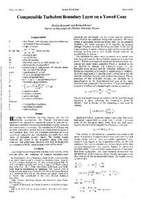
26
Original verification of Morkovin scaling of compressible streamwise turbulence profiles. From Morkovin (1961) . . . . . . . . . . . . . . . . . . . .
27
2.7
Survey of compressible streetwise turbulence data in Morkovin scaling . . .
31
2.8
Mach 5 Morkovin scaled turbulence results of Tichenor et al. (2013) . . . .
32
2.9
Preliminary hypersonic PIV results of Sahoo et al. (2009a) . . . . . . . . . .
33
2.10 Examples of hairpin vortices. From Adrian et al. (2000b) and Zhou et al. (1999) . . . . . . . . . . . . . . . . . . . . . . . . . . . . . . . . . . . . . . . .
36
2.11 Illustration of the concept of nested hairpin packets. From Adrian et al. (2000b) . . . . . . . . . . . . . . . . . . . . . . . . . . . . . . . . . . . . . . . 3.1
39
Illustration of basic 2D2C PIV setup and cross-correlation analysis. From Raffel (2007) and Adrian (2005) . . . . . . . . . . . . . . . . . . . . . . . . . xiii
43
3.2
Demonstration of a method for estimating the random error of PIV. From Discetti et al. (2013). . . . . . . . . . . . . . . . . . . . . . . . . . . . . . . . .
48
3.3
Estimation of random error as a function of interrogation window size . . .
49
3.4
Effect of limited resolution on measured turbulence by PIV. From Spencer and Hollis (2005). . . . . . . . . . . . . . . . . . . . . . . . . . . . . . . . . .
3.5
51
Effect of limited PIV resolution on estimation of the integral lengthscale. From Spencer and Hollis (2005). . . . . . . . . . . . . . . . . . . . . . . . . .
53
3.6
Pictures of stable boundary layer tunnel heater power and control apparatus
58
3.7
Picture of completed stable boundary layer tunnel . . . . . . . . . . . . . . .
59
3.8
Schematic of the measurement setup for stably stratified boundary layer measurements. . . . . . . . . . . . . . . . . . . . . . . . . . . . . . . . . . . .
3.9
60
Pictures of the thermocouple rake for the measurement of mean temperature profiles . . . . . . . . . . . . . . . . . . . . . . . . . . . . . . . . . . . . .
61
3.10 PIV setup for the stably stratified boundary layer in operation. . . . . . . . .
62
3.11 Plan view of HyperBLaF wind tunnel. From Baumgartner (1997). . . . . .
64
3.12 Operating conditions of HyperBLaF wind tunnel . . . . . . . . . . . . . . .
65
3.13 Operating conditions of HyperBLaF air ejector system . . . . . . . . . . . .
66
3.14 Effect of poor hypersonic wind tunnel startup on mean velocity profiles . .
67
3.15 HyperBLaF wind tunnel modifications . . . . . . . . . . . . . . . . . . . . .
71
3.16 Hypersonic turbulent boundary layer test plate . . . . . . . . . . . . . . . . .
72
3.17 Details of HyperBLaF wind tunnel test section configured for PIV . . . . .
74
3.18 Fluidized bed particle seeder for HyperBLaF wind tunnel . . . . . . . . . .
75
4.1
PIV setup for stably stratified boundary layer turbulence measurements . .
82
4.2
Range of stable boundary layer test conditions - Riδ vs. Reθ . . . . . . . . .
84
4.3
Neutral - Mean velocity profiles (inner coordinates) . . . . . . . . . . . . . .
89
4.4
Neutral - Turbulent shear stress . . . . . . . . . . . . . . . . . . . . . . . . . .
91
4.5
Neutral - Skin friction estimates . . . . . . . . . . . . . . . . . . . . . . . . .
92
xiv
4.6
Neutral - Streamwise and wall-normal variance . . . . . . . . . . . . . . . .
96
4.7
Stable - Mean velocity profiles . . . . . . . . . . . . . . . . . . . . . . . . . . 101
4.8
Stable - Mean temperature profiles . . . . . . . . . . . . . . . . . . . . . . . . 101
4.9
Stable - Gradient Richardson number profiles . . . . . . . . . . . . . . . . . 104
4.10 Stable - Turbulent stresses scaled by freestream velocity . . . . . . . . . . . 106 4.11 Effect of thermal stability on the anisotropy ratio . . . . . . . . . . . . . . . 108 4.12 Stable - Mean velocity profiles, inner scaling . . . . . . . . . . . . . . . . . . 112 4.13 Stable - Turbulent stresses in classical outer scaling . . . . . . . . . . . . . . 114 5.1
Change instantaneous streamwise velocity fields with increasing stratification124
5.2
Example of instantaneous neutrally stratified structure, including hairpin vortex signatures and packets . . . . . . . . . . . . . . . . . . . . . . . . . . . 128
5.3
Changes to instantaneous boundary layer structure with increasing stratification - Smooth wall . . . . . . . . . . . . . . . . . . . . . . . . . . . . . . . . 134
5.4
Detail of hairpin vortex signatures in stably stratified boundary layers Smooth wall . . . . . . . . . . . . . . . . . . . . . . . . . . . . . . . . . . . . . 135
5.5
Changes to instantaneous boundary layer structure with increasing stratification - Rough wall . . . . . . . . . . . . . . . . . . . . . . . . . . . . . . . . 138
5.6
Detail of hairpin vortex signatures in stably stratified boundary layers Rough wall . . . . . . . . . . . . . . . . . . . . . . . . . . . . . . . . . . . . . 139
5.7
Examples of alternate structures that appear at high stratification - Smooth wall . . . . . . . . . . . . . . . . . . . . . . . . . . . . . . . . . . . . . . . . . 141
5.8
Effect of stratification on the mean swirl of prograde and retrograde vortices in outer scaling . . . . . . . . . . . . . . . . . . . . . . . . . . . . . . . . . . . 144
5.9
Effect of stratification on the standard deviation of signed swirl in outer scaling . . . . . . . . . . . . . . . . . . . . . . . . . . . . . . . . . . . . . . . . 145
5.10 Effect of stratification and surface roughness on space fractions of signed swirl . . . . . . . . . . . . . . . . . . . . . . . . . . . . . . . . . . . . . . . . . 147 xv
5.11 Effect of stratification and wall-normal distance on the PDF of signed swirl 150 5.12 Effect of stratification on smooth-wall Ruu spatial correlation . . . . . . . . . 152 5.13 Effect of stratification on smooth-wall Rww spatial correlation . . . . . . . . 153 5.14 Effect of stratification on rough-wall Ruu spatial correlation . . . . . . . . . . 154 5.15 Effect of stratification on rough-wall Rww spatial correlation . . . . . . . . . 155 5.16 Effect of surface roughness and thermal stability on the length scales of Ruu spatial correlation . . . . . . . . . . . . . . . . . . . . . . . . . . . . . . . . . 157 5.17 Effect of surface roughness and thermal stability on the length scales of Rww spatial correlation . . . . . . . . . . . . . . . . . . . . . . . . . . . . . . . 158 5.18 Effect of surface roughness and thermal stability on the aspect ratio of Ruu spatial correlation . . . . . . . . . . . . . . . . . . . . . . . . . . . . . . . . . 159 5.19 Estimation of the angle of hairpin packets from the aspect ratio of the Ruu spatial correlation . . . . . . . . . . . . . . . . . . . . . . . . . . . . . . . . . 161 5.20 Effect of thermal stability and surface roughness on the characteristic angle of the Ruu spatial correlation . . . . . . . . . . . . . . . . . . . . . . . . . . . 164 5.21 Influence of surface roughness and thermal stability on integral lengths . . . 167 5.22 Effect of stratification on smooth-wall Ruu temporal correlation . . . . . . . 169 5.23 Effect of stratification on smooth-wall Rww temporal correlation . . . . . . . 170 5.24 Effect of stratification on rough-wall Ruu temporal correlation . . . . . . . . 171 5.25 Effect of stratification on rough-wall Rww temporal correlation . . . . . . . . 172 5.26 Effect of stratification on quadrant contributions to the turbulent shear stress - Smooth wall . . . . . . . . . . . . . . . . . . . . . . . . . . . . . . . . 176 5.27 Effect of stratification on quadrant contributions to the turbulent shear stress - Rough wall . . . . . . . . . . . . . . . . . . . . . . . . . . . . . . . . . 177 5.28 Effect of stratification on the ratio of Q2 and Q4 contributions . . . . . . . . 178 5.29 Effect of stratification on quadrant contribution space fractions - Smooth wall181 5.30 Effect of stratification on quadrant contribution space fractions - Rough wall 182 xvi
5.31 Effect of stratification on the angle of u-w joint-PDF . . . . . . . . . . . . . 184 6.1
Example of Peak locking on global displacement histogram. From Christensen (2004) . . . . . . . . . . . . . . . . . . . . . . . . . . . . . . . . . . . . 198
6.2
Example of effect of peak locking on turbulent statistics. From Angele and Muhammad-Klingmann (2005) . . . . . . . . . . . . . . . . . . . . . . . . . . 200
6.3
Hypersonic PIV Code Comparison - Global histograms . . . . . . . . . . . . 208
6.4
Hypersonic PIV Code Comparison - Mean velocity . . . . . . . . . . . . . . 210
6.5
Hypersonic PIV Code Comparison - Turbulence . . . . . . . . . . . . . . . . 211
6.6
Hypersonic PIV Code Comparison - WIDIM overlap factor . . . . . . . . . 213
6.7
Laser pulse separation uncertainty - varying flashlamp to Q-switch trigger separation . . . . . . . . . . . . . . . . . . . . . . . . . . . . . . . . . . . . . . 217
6.8
Laser pulse separation uncertainty - varying flashlamp voltage . . . . . . . . 218
7.1
Variation in spherical particle drag relative to Stokes drag . . . . . . . . . . 227
7.2
Variation in spherical particle drag relative to the Schiller-Neumann drag relation . . . . . . . . . . . . . . . . . . . . . . . . . . . . . . . . . . . . . . . 229
7.3
Analysis of particle response across a shock, following pathlines . . . . . . 230
7.4
Example of simulated shock response at reference conditions . . . . . . . . 232
7.5
Variation in frequency response with particle size and density for a particle crossing a shock at reference conditions . . . . . . . . . . . . . . . . . . . . . 234
7.6
Variation in normalized particle response with shock strength at reference conditions . . . . . . . . . . . . . . . . . . . . . . . . . . . . . . . . . . . . . . 236
7.7
Variation in normalized particle response with shock strength, considering a range of conditions typical of high Mach number wind tunnels . . . . . . 237
7.8
Analysis of the sensitivity of particle response to shock strength as a function of freestream Mach number . . . . . . . . . . . . . . . . . . . . . . . . . 239
7.9
Particle responses to small disturbances . . . . . . . . . . . . . . . . . . . . . 240 xvii
7.10 Estimate of the variation in frequency response across Mach 7.4 boundary layer . . . . . . . . . . . . . . . . . . . . . . . . . . . . . . . . . . . . . . . . . 243 8.1
Effect of over-tripping on the wake component of incompressible boundary layers as compiled by Coles (1962). . . . . . . . . . . . . . . . . . . . . . . . 249
8.2
Strength of the wake component in compressible turbulent boundary layers as compiled by Fernholz and Finley (1980) . . . . . . . . . . . . . . . . . . . 250
8.3
Dimensions of test plate and leading edges employed in hypersonic tripping study . . . . . . . . . . . . . . . . . . . . . . . . . . . . . . . . . . . . . . . . . 252
8.4
2D and 3D tripping devices employed in hypersonic tripping study. . . . . . 253
8.5
Analytic estimates for leading edge laminar boundary layer viscous interaction . . . . . . . . . . . . . . . . . . . . . . . . . . . . . . . . . . . . . . . . 257
8.6
Effect of tripping on van Driest transformed mean velocity profiles in inner scaling . . . . . . . . . . . . . . . . . . . . . . . . . . . . . . . . . . . . . . . . 261
8.7
Detail of tripping effect on wake component of mean velocity profiles . . . 262
8.8
Wake strength variation with trip size and Reynolds number . . . . . . . . . 263
8.9
Effect of tripping on Morkovin scaled streamwise turbulence profiles . . . . 264
8.10 Surface flow visualization of the wakes of cylindrical post tripping devices 266 9.1
Assessment of hypersonic PIV data: Mean velocity profiles . . . . . . . . . 274
9.2
Assessment of hypersonic PIV data: Morkovin (outer) scaled turbulence profiles . . . . . . . . . . . . . . . . . . . . . . . . . . . . . . . . . . . . . . . . 275
9.3
Assessment of hypersonic PIV data: (a) inner (b) semi-local streamwise turbulence scalings . . . . . . . . . . . . . . . . . . . . . . . . . . . . . . . . . 276
9.4
Instantaneous streamwise velocity fields in a hypersonic boundary layer obtained using PIV . . . . . . . . . . . . . . . . . . . . . . . . . . . . . . . . . 279
A.1 Thermally stratified wind tunnel drawings: overview of modifications . . . 283
xviii
A.2 Thermally stratified wind tunnel drawings: location of thermocouples and heating elements. . . . . . . . . . . . . . . . . . . . . . . . . . . . . . . . . . . 284 A.3 Thermally stratified wind tunnel drawings: mounting locations for upstream heated plate. . . . . . . . . . . . . . . . . . . . . . . . . . . . . . . . . 285 A.4 Thermally stratified wind tunnel drawings: mounting locations for downstream heated plate. . . . . . . . . . . . . . . . . . . . . . . . . . . . . . . . . 286 A.5 Thermally stratified wind tunnel drawings: upstream support framing, outer frame dimensions. . . . . . . . . . . . . . . . . . . . . . . . . . . . . . . 287 A.6 Thermally stratified wind tunnel drawings: upstream support framing, cross member dimensions. . . . . . . . . . . . . . . . . . . . . . . . . . . . . 288 A.7 Thermally stratified wind tunnel drawings: downstream support framing, outer frame dimensions. . . . . . . . . . . . . . . . . . . . . . . . . . . . . . . 289 A.8 Thermally stratified wind tunnel drawings: downstream support framing, cross member dimensions. . . . . . . . . . . . . . . . . . . . . . . . . . . . . 290 A.9 Thermally stratified wind tunnel drawings: non-heated side plates. . . . . . 291 A.10 Thermally stratified wind tunnel drawings: leading edge. . . . . . . . . . . . 292
xix
Chapter 1 Introduction 1.1
Atmospheric and Hypersonic boundary layers: Why are they important? How do they differ?
Experiments are reported which examine the effects of density gradients on turbulent boundary layer structure. Examples of such flows are numerous, including the movement of fluid over plate heat exchangers, salinity stratification in the ocean beneath ice, the atmospheric surface layer (ASL), or the flow around high-speed aircraft and spacecraft. This thesis will focus on the final two examples in detail, examining the changes to the structure of the atmospheric surface layer under strong, statically stable, density gradients, as well as investigating the scaling of high speed turbulent boundary layers as the Mach number is increased from the supersonic to hypersonic regimes. The effects of density gradients on turbulence is known to be significant and very different in each case. The atmospheric surface layer is more often stratified than not, with strong surface heating by the sun during the day and radiative cooling at night, corresponding to unstable and stable conditions, respectively. With instability, large buoyant plumes are known to increase turbulent mixing, while under stable conditions turbulence is damped, sometimes becoming highly intermittent (Stull, 1988). Heat fluxes to the surface are also reduced un1
der stable conditions. For these and many other reasons to be discussed, the strong stably stratified regime remains a challenge to scaling theories, and its implementation in global climate models is currently semi-empirical, with factors tuned to provide physically recognizable weather patterns and not based on theory (King et al., 2001). This approach is especially problematic in the polar regions, where the flow of warmer air over the cold icepack couples the atmospheric turbulence and the surface heat flux, thereby determining melting rates and macroscopic temperatures. To highlight this complexity, King et al. (2001) conducted a coarse simulation (first grid level approximately 20m above the ground) of the airflow over the Antarctic using four commonly used stable boundary layer parameterizations. They found a variation of over 10○C in winter average temperature, and in a couple of cases encountered runaway surface cooling, which is non-physical. Little is understood about the mechanistic changes to flow structure associated with strong thermal stability, necessary in the formulation of better models. Because atmospheric measurements are often difficult due to the unsteadiness of conditions and the small magnitude of surface fluxes, much can be gained through laboratory experiment which can provide greater control of boundary conditions as well as information about the spatial variation in coherent structures using measurement techniques such as particle image velocimetry (PIV), employed in this thesis. Likewise, our understanding of compressible, high Mach number boundary layers is limited due to the lack of available data and the difficulty of experiments or simulations. This lack of understanding compromises the design of high speed vehicles, as turbulent boundary layers determine the aerodynamic drag and heat transfer. Without a sufficiently accurate understanding of the flow physics, large safety margins must be enacted, increasing weight and cost. Modern vehicle design increasingly relies on flow simulations, which are cheaper and provide a greater amount of information than full scale tests, but without further data to validate the models upon which these codes are based, progress remains uncertain. 2
At high speeds the density gradients are not generated primarily through changes in wall-temperature (although this complication can be included) but through the viscous heating caused by slowing the flow from high speed to zero within the small thickness of the boundary layer. In contrast to the atmospheric surface layer, buoyancy effects are negligible at supersonic Mach numbers, and turbulence is expected to scale with changes in fluid density. This expectation is a consequence of Morkovin’s Hypothesis, which postulates that high speed turbulence structure in zero pressure-gradient turbulent boundary layers remains largely the same as its incompressible, neutrally stratified counterpart. While some experimental verification exists at supersonic speeds up to Mach 5, there is little data at higher, hypersonic, speeds. At such speeds, Morkovin’s hypothesis is potentially invalidated by non-negligible density and pressure fluctuations which increase with Mach number. In addition, the fluctuating Mach number, M ′ , defined as the ratio of the fluctuating velocity field to the local speed of sound, also increases. At approximately Mach 5 (depending on the heat transfer condition), M ′ will approach a value of one somewhere in the boundary layer (Smits and Dussage, 2005). As a result, turbulent fluctuations will become locally supersonic relative to the surrounding flow, likely creating local shocklets that may be the source of significant pressure fluctuations. The Mach number at which these effects invalidate Morkovin’s Hypothesis has not been experimentally determined. DNS/LES simulations are providing ever increasing insight into these high speed flows, and they will become increasingly important for the design of vehicles. However, the experimental database against which these computations are validated is extremely sparse (see for example the recent review by Smits et al. (2009)). However, the capability of the cameras and lasers required for PIV has advanced to the point where the direct measurement of spatially varying velocity fields can be attempted in high speed flows, providing significantly greater information than previously possible. In this thesis, these two distinct flows are studied in detail. In both cases, advanced PIV methods will be used to study changes to turbulent coherent structures, length scales and 3
deviations of statistics from current scaling theories. Such measurements are challenging, for reasons detailed in the following section. Thus an assessment is first undertaken of the limitations of PIV, as applied to the measurement of turbulence.
1.2
Difficulties obtaining accurate data / benefits of laboratory scale measurements
While the need for additional data within the ASL and in hypersonic boundary layers has been recognized for some time, such experiments face many challenges. For high speed flows, full scale experiments are extremely expensive and usually constrained to surface measurements and not those of the fluctuating velocity field. For the ASL, experiments are hampered by the transience of any given flow condition, following the diurnal cycle, with stratification levels that rarely remain constant for long. Coupled to this are unknown history effects and questions with regard to topography and upstream fetch. The ASL can also be constrained from above by a number of different thermal and velocity boundary conditions, and it can sometimes entrain turbulence from above. As measurements are taken near the ground, these boundary conditions are often not well characterized. At laboratory scale, the study of these flows requires the construction of dedicated wind tunnel facilities. These facilities often have significant space and power requirements as both heating or cooling elements are needed. In addition, hypersonic wind tunnels often require compressed gases for operation, necessitating additional infrastructure. That being said, once constructed, these wind tunnels allow the proper control of boundary conditions and acquisition of a significantly more detailed information. A new thermally stratified lowspeed wind tunnel was constructed to conduct the thermally stable experiments described in this thesis. The hypersonic experiments were conducted in Princeton Gas Dynamics lab’s HyperBLaF wind tunnel which employs compressed air to run for up to 90s at Mach
4
8. Significant modifications were required to introduce seeding particles to conduct PIV and to reduce flow disturbances, improving tunnel start-up reliability. Obtaining the correct conditions is only half the problem, since the measurements themselves are also difficult. The primary challenge is a result of the co-dependence of the fluctuating velocity and temperature fields as well as the required sensitivity of such measurements. For instance, while turbulence data have previously been acquired in hypersonic turbulent boundary layers using hot-wire anemometry, the hot-wire is sensitive to fluctuations in mass flow and not velocity, as the temperature field is also fluctuating. To separate out the velocity fluctuations from the mass flow fluctuations, the Strong Reynolds Analogy (SRA) is often used, which relates velocity and temperature fluctuations, although its general validity has been called into question (Smits and Dussage, 2005). Combined with a limited frequency response, the resulting hot-wire data are highly variable, especially in the near-wall region (see Sec.2.2.3). Within the atmosphere, heat and momentum fluxes are conventionally acquired with sonic-anemometers. The reductions in these fluxes, as a result of thermal stability, taxes the spatial and temporal resolution of such instrumentation. Laboratory hot-wire experiments in thermally stratified flows suffer from the same mixed mode sensitivity as experienced in hypersonic experiments. In this thesis, PIV will be used to directly measure the fluctuating velocity field. In this way, spatially varying flow structures can be directly identified and compared with previous studies examining neutrally stratified incompressible boundary layers. The mean density gradient is obtained through the Walz relation (see Sec.2.2.1) in the hypersonic case, and through the use of a thermocouple rake for the low-speed thermally stable boundary layer. In this way, scaling of turbulence with respect to the mean density gradient can be examined for both flows. Future work will address the simultaneous measurement of fluctuating temperature using a new Nano-scale sensor (Arwatz et al., 2014).
5
Chapter 2 Background In this thesis different coordinate systems will be used, depending on the type of boundary layer being discussed. For all discussions of hypersonic boundary layer research, the wallnormal distance and velocity will be denoted by y, V, respectively. For all discussions of thermally stratified boundary layers, the wall-normal distance and velocity will be denoted by z, W, respectively, following the conventions of the atmospheric community.
2.1
Thermally Stable Boundary Layers
In this section, some important aspects of thermally stable boundary layers will be reviewed, beginning with a discussion of measures of stability, followed by delineation of different regimes found within the atmospheric surface layer. At its most basic level, a stably stratified boundary layer can be separated into two stratification regimes, weak and strong stability, which obey different scaling laws and are separated by a level of critical stratification. The evidence for this critical stratification and previous estimates of its value are discussed. The section finishes with a description of previous experimental results with which the current study will be compared.
6
2.1.1
Monin-Obukhov Similarity Theory (MOST)
By far the most common scaling theory to account for buoyancy effects on turbulent statistics was presented by Monin and Obukhov (1954), subsequently known as Monin-Obukhov Similarity Theory (MOST). They hypothesized that, assuming a fluid layer of constant heat and momentum flux, any turbulent quantity could only depend on five parameters; the wall-normal distance, z, the momentum flux, uw, the fluid density, ρ, the ratio of gravity and ambient temperature, g/T a , and the vertical turbulent heat flux, wθ. Here, lower case letters u, v, w represent velocity fluctuations, relative to the mean, in all three coordinate directions and θ is the fluctuating temperature. A line over a variable signifies that it is time-averaged quantity. Through dimensional analysis it can be shown that the any appropriately scaled turbulent quantity should be a single valued function of, z/L, where L is the Monin-Obukhov length defined as,
L = −u3τ / (κ
g wθ) , Ta
(2.1)
is a constant within the constant flux layer and 1/2
uτ ≈ −uw0 T∗ =
H0 −wθ =− uτ κρ0C p0 uτ
Friction velocity
(2.2)
Friction temperature
(2.3)
H0 = κρ0C p0 wθ Subscripts
0
(2.4)
represent surface values. The variables ρ, C p , H represent the fluid density,
specific heat at constant pressure and heat flux, respectively. κ is the von K´arm´an constant. The appropriate scaling parameters are thus z, uτ and T ∗ . Turbulent quantities such as the gradients in mean velocity and temperature are thus functions of the similarity parameter, z/L. Suitably non-dimensionalized MOST functions
7
for common turbulent quantities are, κz ∂U z =1+β uτ ∂z L κz ∂T z φh (z/L) = = 1 + βT T ∗ ∂z L
φm (z/L) =
for z/L > 0
Mean velocity profile
(2.5)
for z/L > 0
Mean temperature profile
(2.6)
Fluctuating wall-normal velocity
(2.7)
Fluctuating temperature
(2.8)
φw (z/L) = σw /uτ φθ (z/L) = σθ / ∣T ∗ ∣
where σw and σθ are the rms values of the wall-normal velocity and temperature, respectively. The linear approximation to the functions φm and φh , with coefficients β and βT , is valid for the stable ABL only. These velocity and temperature gradient functions (Eq.2.5 and 2.6) correspond to the neutrally buoyant log-law for zero stratification, thus φm (0) = φh (0) = 1. A number of studies have evaluated the functional form of these similarity equations from atmospheric data and the linear form of the velocity and temperature gradient functions, φm and φh has been confirmed under stable conditions. The most widely used MOST functions are the Businger-Dyer relationships, for which β = βT = 5 (Stull, 1988). Laboratory data have suggested φm and φh are better fit to a power law (Arya and Plate, 1969). This may be evidence of a Reynolds number influence on these functions. For z/L > 1, these relations are known to break down and atmospheric data shows significant scatter (Mahrt, 1998). This is partially due to measurement difficulties and turbulence intermittency. MOST also breaks down in regions where the fluxes are not constant. In the weakly stratified atmosphere, the constant flux, inertial layer covers the majority of the boundary layer, outside the roughness sublayer and so MOST is valid. As stratification increases, this regions shrinks, confining the region within which MOST is valid to a region closer to the surface, as will be discussed in the following section. These formulations also suffer from self-correlation, with the wall distance, z being present in the functions above and in the stability parameter, z/L. This tends to make the 8
evaluation of their functional form more difficult for noisy data as even uncorrelated data will suggest some functional dependence.
2.1.2
Other measures of stability
A number of other parameters are used to describe the extent of thermal stratification on turbulent statistics, with different formulations used depending on the amount and type of data available, or the flow under discussion. One of the most common parameters is the local gradient Richardson number,
Ri =
g ∂T /∂z N2 = T (∂U/∂z)2 ( ∂U )2 ∂z
(2.9)
which describes the relative influence of the stabilizing effect of buoyancy and the destabilizing effect of shear. Here, T is the mean temperature, U is the mean velocity, z is the √ wall-normal distance, g is the gravitational constant and N = − (g/T ) ∂T /∂z is the BruntV¨ais¨al¨a frequency, which is a measure of static stability. It can be seen that MOST implies that Ri is also a single valued function of z/L as
Ri =
z φh = f1 (z/L) L φ2m
(2.10)
and thus, if turbulence can be collapsed on a single function of Ri, MOST can also be assumed to be valid. This is especially useful for laboratory experiments as measurement of the fluxes necessary to estimate L can be difficult. Also commonly used, especially when discussing laboratory experiments, is the bulk Richardson number, Riδ =
gδ ∆T 2 T ∞ U∞
(2.11)
which is equivalent to the gradient Richardson number evaluated with an estimate of the mean gradients. Here, ∆T is the temperature difference across the layer, T ∞ is 9
the freestream temperature, U∞ is the freestream velocity, and δ is the boundary layer thickness. Within the ASL community, the bulk Richardson number is primarily used to estimate its height. Still further measures of stratification are the stress and flux Richardson numbers,
Ri s =
(g/T 0 )uθ w2 ∂U/∂z
Ri f =
(g/T 0 )wθ Kh φm ≈ Ri = Ri uw∂U/∂z Km φh
(2.12)
where, uθ and wθ represent the streamwise and wall-normal turbulent heat fluxes (Arya, 1974; Stull, 1988). These measures originate from the ratio of buoyant destruction to mechanical production terms within the equations for turbulent kinetic energy (TKE) and the momentum flux and turbulent shear stress, uw, respectively, and are thus directly related to properties of the turbulence. The flux Richardson number can be related to the gradient Richardson number through the turbulent Prandtl number, Prt = Kh /Km , which is the ratio of eddy diffusivities of heat and momentum and can be related to the Monin-Obukhov functions. The behavior of this ratio with increasing stratification is still contested (Zilitinkevich et al., 2013; Katul et al., 2014). Most recently, great promise has been shown using the ratio of turbulent kinetic energy to turbulent potential energy as a measure of stratification (Zilitinkevich et al., 2013). Once again, however, evaluation of this parameter requires significantly greater data than that available in laboratory experiments and so it will not be evaluated in this thesis.
2.1.3
Stable boundary layer regimes
The stable atmospheric boundary layer can be divided into a number of physical layers that change as a function of stratification, as laid out by Mahrt (1999) and shown in Fig.2.1. MOST requires a region of approximately constant heat and momentum flux, which is situated above the roughness sublayer and labeled the surface layer in Fig.2.1. With increasing stability, this region is known to shrink in wall-normal extent, potentially lying 10
266
L. Mahrt
Figure 2. Different stable boundary-layer regimes as a function of stability. The vertical dashed line indicates the value of z/L Figureto 2.1: Regimes of the thermally stable atmosphere as a function of MOST parameter corresponding maximum downward heat flux.
z/L. From Mahrt (1999). In practice, the aerodynamic temperature is replaced with the temperature of the solid surface. In models, the surface can be computed from surface energy balance externally specified belowtemperature the lowest observation level at highthestratification, making the or determination of the as a boundary condition. Use of the surface temperature in place of the aerodynamic temperature redefines the surface fluxes problematic. roughness length for potentially heat which is then computed from data using Eqs. 2 and 3, the observed fluxes and the specified stability functions 'h (z/L) and 'm (z/L). Above the surface layer, the fluxes depend height andmomentum thus MOST similarity is not The thermal roughness length is usually specified to beon less than the roughness length although observations over a variety of surfaces collectively suggest that the thermal roughness is not closely related valid. It is theorized however, that if the Monin-Obukhov length is reformulated in terms of to the momentum roughness length and is sometimes erratic and unpredictable (see Sun and Mahrt (1995); and papers surveyed Mahrt (1996)). Unfortunately, of z0T from in the the local fluxes,inthe same functional forms are calculations still approximately validobservations for z/Λ, where Λ stable atmospheric boundary layer are almost nonexistent. Sun (1997) finds that in the stable boundary layer over a simple grass surface, z0T is uncorrelated with with z0 butlocal is generally smaller than z0 local-scaling. and sometimesAt reaches is the Monin-Obukhov length evaluated fluxes. This is termed extremely small values. The erratic behavior of z0T probably indicates that applying Monin–Obukhov distances even further the surface, equivalently, at even higherCertainly, stratification similarity to compute the heatfrom flux using a singleor surface temperature is flawed. overlevels, complicated surfaces, multiple surface temperatures are required and the use of a single surface temperature is inadequate. a ‘z-less’ stratification exist which can be derived from the asymptotic limit of This topic is beyond the scoperegime of this may review. The erratic behavior of the thermal roughness length led Mahrt et al. (1997a) and Sun et al. (1997) the linear MOST functions for large z/Λ, where local conditions are independent of their to eliminate the thermal roughness length as an unknown by equating it with the momentum roughness length.distance This defines aerodynamic temperature which musttothen be related to practicalextent observable fromthe thesurface surface. Each of these regimes are known shrink in wall-normal temperatures. The problem has not been closed in a general way. In the proceed with the of usual replacement the aerodynamic temperature with the temfor following, increasingwe stability until none these similarity of theories remain valid. perature of the surface and return to the early practice of equating the thermal roughness length to the momentum Toroughness simplify length: this picture, the stable atmosphere is conventionally divided into only z0T = z0 . (6) two regimes instead; the weakly stable regime, where turbulence dominates and MoninThe philosophy is to be as simple as possible until more sophisticated formulations can be fully justified. similarity is valid for aUsing least (6) a portion ofvalue the layer, and the strongly stablefor regime, This isObukhov the approach followed below. and the of the surface temperature the surface aerodynamic temperature, the heat flux can be predicted from (2)–(3), provided that the stability functions where MOST fails and other features such as the detachment of turbulence from the surface, and are known. h m gravity waves, or Kelvin-Helmholtz instabilities appear. As indicated by (Mahrt, 1999), the 2.1. Stability 11 Functions The usual route for estimating the stability functions is first to determine the dependence of the nondimensional profile functions 'h (z/L) and 'm (z/L) and then to integrate them vertically. The advantage of determining 'h (z/L) and 'm (z/L) is that they are calculated from data in the surface layer independently
use of only two regimes is most likely an oversimplification. Additional features such as clear-air radiative cooling, low-level jets, surface heterogeneity, and mesoscale motions are also known to strongly influence atmospheric results where there is a high degree of stratification. A concise definition of the strongly stable regime remains difficult. Some of its properties were summarized by Mahrt (1999), including: • Turbulence intermittency near the surface, where turbulence can occur only in bursts. • Emergence of gravity waves and Kelvin-Helmholtz instabilities, whose contributions to turbulent statistics must be disentangled from those of turbulence. • Invalidation of MOST or, for atmospheric observations, flux divergence below the lowest observational level. MOST is known to break down for z/L ≈ 1 Mahrt (1999) also describes boundary layers of upside down character, where turbulence is almost completely damped near the surface but remains aloft after the turbulence can no longer support the required downward heat flux. In this situation, counter-gradient fluxes are observed and thus the traditional flux-gradient transport turbulence model breaks down. It is likely that this elevated turbulence is intermittently coupled to the surface, as the near-wall damping of turbulence will result in the buildup of shear, which can break down to turbulence once more, creating a cycle. Within the atmosphere the upside down, strongly stable boundary layer is not universal, with the region of maximum turbulence sometimes seen at the top of the inversion layer, or occurring as the result of a layer of residual turbulence left over from earlier unstable conditions (Mahrt, 1999). This type of upside down boundary layer was first observed in laboratory experiments by Ohya et al. (1996), who noted a peak in the velocity variances and vertical heat flux in the outer layer. They also delineated between the weakly and strongly stable regimes by the collapse of near wall turbulence. For their data, this collapse occurred at a critical bulk Richardson number of close to 0.25. The local gradient Richardson number was also seen 12
to be greater than 0.25 in the near-wall region within the strongly stable regime (as they defined it). In this thesis we will critically examine these observations, among others, as well as the notion of a critical Richardson number and the definition of the strongly stable regime. The existence and value of the critical Richardson number separating the weakly and strongly stable regimes has been contested for some time, and is reviewed in the following section. Such a critical value is likely to be an oversimplification, as is the separation of the stable boundary layer into strongly and weakly stable regimes, as we shall see.
2.1.4
The critical Richardson number
The most often quoted critical Richardson number, of which there are many, comes from linear stability theory. Miles (1961) and Howard (1961) determined that a laminar, steady, inviscid flow would remain laminar to small perturbations for Ri > 1/4. This is a sufficient condition that was first predicted by Taylor (1931) and later verified experimentally by Scotti and Corcos (1971). It should be noted, however, that unsteadiness has been shown to delay instability to Richardson numbers greater than 1/4 (Majda and Shefter, 1998), possibly helping to explain some of the variability in the atmospheric data due to its unsteadiness inherent in the diurnal cycle. Ohya et al. (1996) observed a critical stratification of approximately 0.25 separating the weakly and strongly stable regimes but the fact that the value determined in this study corresponds so closely to Miles-Howard theory is not automatic. Although the condition, Ri > 1/4, has been shown to be a sufficient condition for the maintenance of laminar flow under certain conditions, it does not necessarily apply to the cessation of turbulence within an already turbulent flow. It should also be noted that the Richardson numbers within the experiment are bulk values instead of the local gradient Richardson number used in the theory.
13
A number of competing analyses present alternate limits. For example, Schlichting (1979) conducted another linear stability analysis of a stratified laminar boundary layer that included viscous effects and a Blasius velocity profile, improving on the analysis of Miles and Howard as the inclusion of viscosity and velocity profile curvature are needed to properly characterize the critical layer. He found that these flows remain stable to small perturbations below a critical Reynolds number that increases quickly with stratification. For Ri > 1/24 ≈ 0.042 it was shown that the flow should remain laminar for any Reynolds number. This was experimentally verified by Schlichting in channel flow. The first analysis of turbulent stratified flows by Richardson (1920) predicted that turbulence would be completely suppressed for Ri > 1 through an analysis of the equations that govern the turbulent fluxes and assuming that steady turbulence would cease if buoyant dissipation exceeded turbulent production. Viscous dissipation was neglected in this analysis and so its validity should be questioned. Recent experimental and observational studies have indicated, however, that this criterion corresponds much more closely to the atmosphere than the more often discussed Miles-Howard result as models of stratified turbulence that use a critical Richardson number as a threshold for the extinction of turbulence have been found to have insufficient mixing if the critical Richardson number Ric < 1 (see Galperin et al. (2007) for discussion). In addition, atmospheric turbulence has been observed to exist for Ri > 1 (Galperin et al., 2007; Zilitinkevich et al., 2013). Canuto (2002) has also demonstrated that the presence of radiative losses and internal gravity waves act to reduce stratification, further increasing the Richardson number required for the suppression of turbulent mixing. Strong stratification has also been observed to increase anisotropy and horizontal mixing even when vertical mixing has been largely suppressed. This observation leads Galperin et al. (2007) to conclude that a single critical Richardson number for the suppression of turbulence does not not exist. An even more recent study by Katul et al. (2014) provides a theoretical basis for the conclusion that the critical gradient Richardson number varies with Reynolds number to the 14
power of 1/3. Thus, it is still unclear if the observation of Ohya et al. (1996) of 0.25 was fortuitous, close to an upper Reynolds number limit, or if indeed intrinsic to the transition to a strongly stable regime at all. Additional estimates of the critical Richardson number have been based on the equations of turbulent kinetic energy, mean square temperature fluctuations, and turbulent heat flux. Ellison (1957) first used this approach, modeling the dissipation terms as the ratio of the turbulent kinetic energy to decay time. Defining the critical stratification as the condition where continuous turbulence cannot be maintained, he arrived at a critical flux Richardson number of Ri f = 0.15. Townsend (1958) based his model on an expected variation in turbulent Prandtl number, and suggested the threshold Ri f = 0.5. Arya (1972) improved on Townsend’s model using Prandtl number measurements, and found a critical value Ri f = 0.15 − 0.25. The definition of ‘critical’ corresponds to the cessation of continuous turbulence and thus these analyses allow for intermittent turbulence above the critical value as the flux Richardson number is a local quantity that for a given flow can fluctuate significantly. These limits have rarely been evaluated due to the difficulty of measuring these fluxes accurately. With so many definitions of the critical Richardson number and different interpretations of the strongly stable regime, it remains difficult to determine which or any of these criteria are correct. Some define ‘critical’ to mean the cessation of turbulence, some the cessation of steady turbulence, and in the case of laboratory flows, the stratification at which nearwall turbulence collapses. Additionally, it is unclear whether global parameters such as the bulk Richardson number are sufficient to characterize the differences between these weakly and strongly stable flows.
2.1.5
Previous experimental results
Experiments examining the effect of stable thermal stratification on turbulent boundary layers are limited, primarily due to the difficult nature of the experiments and the unique 15
nature of the required wind tunnels. Fluctuating velocity and temperature measurements are conventionally acquired in a point-wise fashion using a combination of hot and coldwire anemometry, the former of which require intricate velocity calibration to compensate for the temperature sensitivity of the wire. Cold-wires, used for fluctuating temperature measurements are also known to have low frequency response (Arwatz et al., 2013). Only a few studies have investigated the simplest form of stratification, involving convection of a uniform freestream temperature over a different, constant, wall temperature (Nicholl, 1970; Arya, 1974; Ogawa et al., 1982, 1985; Ohya et al., 1996; Ohya, 2001). Further studies have examined the effects of a capping density interface (Piat and Hopfinger, 1981; Ohya and Uchida, 2004), a linear temperature profile (Ohya and Uchida, 2003), or a simulated low-level jet (Ohya et al., 2008), highlighting the effects of different stratification profiles. These studies demonstrated that thermal stratification significantly suppresses turbulent fluxes and stresses, and produce a progression of the velocity profile towards a more laminar shape. Comparison between these studies has been significantly complicated by 2 the inability to vary both Reynolds and Richardson numbers independently, as Riδ ∼ δ/U∞
and for a given fetch, Reδ ∼ δU∞ and boundary layer thickness is significantly altered by stability. As a result, it has been difficult to tease out the competing effects of Reδ and Riδ on turbulent statistics. Arya (1974) was the only study to present the mean velocity and temperature profiles in semi-logarithmic inner scaling, thus allowing for a comparison of the stably stratified mean velocity profile with the neutrally stratified log-law. In this scaling, velocities are assumed √ to scale with the friction velocity, uτ = τw /ρw , and distances are assumed to scale with the viscous length scale, νw /uτ , where τw is the wall shear stress and ρw , and νw are the fluid density and kinematic viscosity evaluated at the wall temperature, respectively. All quantities in this scaling will be given the superscript + . The friction velocity and temperature were determined from the near wall maximum in the turbulent heat and momentum fluxes, 16
Buoyancy eSfeects in a horizontal boundary layer
327
35
30
25
2C
s" IS 1:
1C
I
I
I
I
I
I
I
1
20
50
100
200
500
1000
2000
u* zlv
Figure 2.2: Effect of both stable and unstable thermal stratification on turbulent boundary layer mean velocity profiles in inner-scaling. # − Riδ = 0.01, △ − Riδ = 0.025, ◻ − Riδ = 0.1. Filled and empty symbols indicate replicates of the same stratification. All other profiles are for unstable thermal stratification, for which there is only a small effect on profile shape. For the purposes of this figure, u∗ = uτ . From Arya (1974). as is common with atmospheric data. The resulting profiles are shown in Fig.2.2. In this (1962)
scaling it was determined that stable stratification initially causes an upward shift in the logarithmic intercept consistent with thickening of the buffer layer, followed by outer layer deviation from the logarithmic slope at progressively lower z+ . In all thermally stable laboratory experiments, the turbulence results were scaled with 01
10
I 20
I
I
I
50
100
200
I 500
I 1000
I
2000
U∞ and δ. In this scaling, Arya (1974) observed clear reductions in turbulence intensity u*Z I V
with increasing stratification, but the profile shape remained relatively constant. Ogawa FIGURE 1. Surface-layer similarity profiles of (a)mean velocity and ( b ) temperature. x , Blom (1970), group IV.
et al. (1982) and Ogawa et al. (1985) measured O A a number O Vof turbulence O Oprofiles acquired
M A of 0pollutant V . dispersion. O in stably stratified flows during their study The data of Ogawa Stability group
I
I1
17
I11
V
VI
VII
et al. (1985) demonstrated an almost uniform collapse of turbulence, in both streamwise and wall-normal directions, followed by relaminarization, which occurred between 0.104 ≤ Riδ ≤ 0.15. Such collapse was not observed by Arya (1974) for Riδ < 0.1 at higher Reynolds numbers. The study of Ogawa et al. (1982) contains only a single stably stratified profile for Riδ = 0.57, much beyond the Richardson number at which turbulence collapsed for Ogawa et al. (1985). In this profile, a small bump was visible in streamwise and wall-normal turbulence in the outer layer turbulence, slightly larger than the freestream turbulence level. This bump was also visible in the more complete study of Ohya et al. (1996), who observed its emergence for Riδ ≈ 0.25, as near wall turbulence was significantly damped. Fig.2.3 summarizes the effect of stratification on the turbulent stresses as observed by Ohya et al. (1996). As previously discussed, Ohya et al. (1996) hypothesized that the collapse of near-wall turbulence and emergence of the outer layer peak signified the transition between weakly and strongly stable regimes. This peak was also seen at high stratification, though weaker, in the follow up study of Ohya (2001) that repeated the earlier experiments but over a rough surface. Very stable cases also demonstrated spectral peaks at much lower frequencies than in the weakly stable regime. In addition, internal gravity waves and Kelvin-Helmholtz instabilities were observed at the highest levels of stratification, and are likely to contribute to the velocity variances under these conditions. It was hypothesized by Ohya et al. (1996) that these non-turbulent, stratified motions might be the cause of the outer layer bump. It seems more likely, however, that the near-wall collapse of turbulence observed by Ohya et al. (1996) is the result of increased local stratification in this region, (see Fig.2.3d), calling into question the nature of their definition of the strongly stable regime. Although the friction velocity, uτ , was known in the majority of these studies, the data were not presented in outer scaling, which would be expected to largely remove Reynolds number effects from velocity statistics. As previously discussed, turbulence quantities were instead presented as a fraction of the freestream velocity or temperature difference, which 18
144
TURBULENCE STRUCTURE IN A STRATIFIED BOUNDARY LAYER
145
YUJI OHYA ET AL.
-
-
Figure 3a. Vertical profiles of the turbulent intensities (r.m.s. values), -component velocityof the ; (a) (b) Figure 3b. Vertical profiles TURBULENCE IN Aline, STRATIFIED 147 turbulent intensities (r.m.s. values), -component velocity 0.1; dash/dotted Ogawa etBOUNDARY al.dashed (1982),line, RiLAYER = 0.57. dashed line, Arya (1975), Ri =STRUCTURE Arya (1975), Ri = 0.1; dash/dotted line, Ogawa et al. (1982), Ri = 0.57. TURBULENCE STRUCTURE IN A STRATIFIED BOUNDARY LAYER
;
155
the floor incorporated an aluminum plate which can face be cooled or heated to any measured with a surface thermocouple and monitored temperatures, , were desired temperature between 5 and 200 C. with a set of thermocouples embedded in the aluminum plate at 30 cm intervals along the center-line. 2.2. EXPERIMENTAL PROGRAM Simultaneous measurements of streamwise and vertical velocities, and , and of fluctuating temperature, , were obtained using thermal anemometry, but Figure 1 shows the experimental arrangement. The boundary layer was artificially adjusting for the large temperature variations in interpreting the sensor response. tripped by a saw-tooth fence with a height of 3.5 cm at the entrance of the test The sensors consist of an -type hot-film probe for velocity and a thin thermocouple section and by 1.2 cm gravel roughness placed on the initial 2 m length of the probe of 0.025 mm diameter for temperature with a separation of 1 mm. The floor. In order to generate stably stratified flows, the surface temperature of the output voltage, , of a constant-temperature anemometer is represented at a sensor aluminum floor over the last 12.2 m of the test section was held at about 3 C and temperature, (given at 250 C), air temperature, , and flow speed, , by that of the ambient air outside the boundary layer at about 50 C. Turbulent boundary layers with free stream velocities of = 0.8–3.02m s 1 were produced. m A IBsummarizes eff These cover a range of stabilities from neutral to strongly stable. Table the Reynolds number, the bulk Richardson number, boundary layer thickness and 2 2 1 2. where eff characteristics cos2 others for each experimental case. Measurements of turbulence in sin Here, A, B and m are constants given by a calibration curve for an ambient the vertical direction were made at a distance of 23.5 m from the saw-tooth fence. temperature. is the yaw angle coefficient of -type hot-film probe and is 2.3. FLOW MEASUREMENT AND DATA ACQUISITION the hot-film angle to the direction of the mean flow. Thus, cross-film data were corrected point by point for temperature fluctuation deviations using the above Figure 9. Vertical profiles of the local gradient Richardson number Ri. relation. Calibration carried out in a(d) special calibration unit with a nozzle and (c) The free streamprofiles velocities, , outside the boundaryflux layers were monitored with a Figure 4a. Vertical of the turbulent fluxes, momentum ; dashed line, Aryawas (1975), mass-flow meter. The velocity manometer. Floor sur- at the nozzle exit is provided by the mass-flow meter. = 0.1. Pitot-static tube in conjunction with an electronic Ristandard in a wind-tunnel experiment (Ri = 0.57) by Ogawa et al. (1982), although they are rather small. The feature of those profiles is that the intensities of and fluctuations approach zero as decreases from the middle of the boundary layer to the bottom. We can find similar profiles of 2 and 2 in the observational studies of Finnigan and Einaudi (1981) and that of 2 in Mahrt (1985). Figure 4a shows the vertical profiles of vertical turbulent momentum flux . For the δstratified flow cases (S1–S5), values are remarkably decreased for 0 6, compared with those for the neutral flow cases (N1, N2). Furthermore, for the strong stability cases (S3–S5), values are almost zero for 0 2. Thus, the profiles exhibit different behaviour for the three distinct stratification regimes. The tendency for the turbulence profiles to separate into three sets is also seen in Figure 3. For the weak stability group (S1, S2), the profiles of are similar to the observational results by Caughey et al. (1979) and Nieuwstadt (1984). For the strong stability group (S3–S5), the profiles of are similar to the results from observational studies by Yamamoto et al. (1979), Finnigan and Einaudi (1981), and
Figure 2.3: Variation of (a) streamwise (b) wall-normal rms velocities (c) shear stresses and (d) gradient Richardson number as measured by Ohya et al. (1996). Cases S1 through S5 are in order of increasing stability (0 ≤ Ri ≤ 1.33) created by decreasing the freestream velocity. The outer layer peak which Ohya et al. (1996) thought to signify the emergence of the strongly stable regime is indicated by the arrows.
19
makes it impossible to differentiate between Reynolds number and Richardson number effects and the comparison between studies difficult. As an example, Ohya et al. (1996)’s used the single profile of Ogawa et al. (1982) (also seen in Fig.2.3) to support the notion that the outer layer peak is intrinsic to the strongly stable regime. When including the neutrally stratified profiles from Ogawa et al. (1982), it becomes clear that the experiments of Ogawa exhibited significantly greater reductions in turbulence than the profiles given by Ohya et al. (1996). If all this data were plotted together, the interpretation of the results is less clear. Many questions also remain with regard to the effects of freestream turbulence intensity and initial conditions. As can be seen in Fig. 2.3, the outer layer peak in w2 intensity is of similar magnitude to the freestream turbulence level, and thus it is unclear if some of the outer layer turbulence peak is related if to disturbances originating from outside the boundary layer. Additionally, many of these previous studies have used fences to trip and artificially thicken the boundary layer at the beginning of the test section. Such disturbances are known to persist for great distances downstream (see Coles (1962)). Proper comparison with the atmosphere requires the evaluation of thermally stratified scaling theories at laboratory scale. Only the data of Arya (1974) has been directly compared with MOST in the study of Arya and Plate (1969). Collapse onto a single curve was extremely tight, though the functional forms were found to be slightly different to atmospheric correlations, with different constants and some debate about the functional forms. Power laws appeared to be more accurate in describing the mean velocity profile at high stability levels than the commonly accepted logarithmic mean velocity profile. Any of these differences could potentially be attributed to differences in Reynolds number or the range of wall-normal positions used in the correlation (0.01 ≤ z/δ ≤ 0.15). Similarly, Ohya et al. (1996) demonstrated the collapse of turbulent quantities with local gradient Richardson number, which should be consistent with MOST as Ri is a function of z/L. A wider range of wall-normal locations were used (0.1 ≤ z/δ ≤ 0.5), including 20
portions of the boundary layer outside of the constant flux region, where MOST should not be valid. No functional forms were fitted or suggested. It thus remains an open question as to what range of wall-normal locations should be included in such a correlation for best correspondence to the atmosphere.
2.1.6
Challenges/Goals
The literature presented above suggest a number of open questions, some of which will be addressed in the following chapters. 1. The effects of stratification on turbulence profiles have not yet been evaluated as they cannot be differentiated from Reynolds number effects when scaling with the freestream velocity. Presenting the results in outer layer scaling may help clarify this problem. 2. It is also unclear if the outer layer peak at high stability is intrinsic to the strongly stable regime, the result of local stratification profiles or the emergence of non-turbulent motions at high stratification. 3. Likewise, the existence of the critical Richardson number is currently debated. If it does exist, its value and concise definition are both unknown. 4. Once the statistical effects of stability are understood, an attempt can be made to determine mechanistic arguments for these changes through an examination of instantaneous coherent structures and their changes with increasing stratification. PIV is ideal for this purpose.
2.2
Hypersonic boundary layers
Hypersonic boundary layers exhibit extreme gradients in fluid density, but in contrast to atmospheric flows, buoyancy effects are negligible (as can be inferred from the definition 21
−2 and thus extremely small in high of the Richardson number which is proportional to U∞
speed flows). In compressible boundary layers, mean density gradients exist primarily due to viscous dissipation, although heat transfer from the wall can also be important. As a result, the use of simple power law temperature profiles is invalidated by the near-wall maximum static temperature. The variation in fluid properties across hypersonic boundary layers is so large that the local Reynolds number varies appreciably across the layer. Reynolds numbers calculated based on fluid properties at the wall can be orders of magnitude smaller than those based on freestream conditions (Fernholz and Finley, 1980). Near-wall heating increases the thickness of the viscous sublayer, making it dependent on Reynolds and Mach numbers as well as the wall heat-transfer rate. Thus the effects of viscosity can be present over a greater proportion of the boundary layer (in terms of y/δ) than in incompressible flows. As a result, it can be difficult to compare compressible boundary layers to their incompressible counterparts as it is unclear how to match Reynolds number, and Reynolds and Mach number effects become intertwined. Compressibility also introduces the potential for significant density and pressure fluctuations, that become more significant as Mach number increases. Nevertheless, a number of scaling theories have been developed to aid comparison with incompressible data. Within the following section these scaling theories will be examined and supporting evidence discussed. The limited number of hypersonic datasets will also be summarized. Further reviews of the state of hypersonic turbulence research and theory can be found in the textbook of Smits and Dussage (2005) and reviews of Roy and Blottner (2006) and Smits et al. (2009).
2.2.1
van Driest scaling of the mean velocity
For a constant Reynolds number, it is now well established that the skin friction coefficient decreases with increasing Mach number (Smits and Dussage, 2005). It is interesting,
22
therefore, to compare the mean velocity profile with the incompressible semi-logarithmic profile, which, in inner scaling is given by U 1 yuτ = ln +B uτ κ ν where κ is the von K´arm´an constant and B is the additive constant. Here, uτ =
(2.13) √
τw /ρ, and
the density and viscosity do not vary with y. To account for the variation in density across the layer, van Driest (1951, 1956) define a transformed velocity U ∗ derived using a temperature-velocity relationship based on the mean energy equation. The transformd velocity is based on an integral variation of the temperature dependence, given by
U∗ = ∫
u
√
u1
Tw du T
(2.14)
where u is the mean streamwise component of velocity, and the suffix 1 denotes a boundary condition at the lower end of the validity range of the log law. The result of the transformation is that zero pressure-gradient turbulent boundary layer data appear to collapse on the incompressible logarithmic profile, with constants unchanged. Fig.2.4 demonstrates the effectiveness of this transformation. Here, the friction √ velocity uτ is given by τw /ρw , and the viscous length scale is νw /uτ , where ρw and νw are the density and kinematic viscosity evaluated at the wall temperature, respectively. It can be seen that the transformation collapses the data on the incompressible logarithmic line. The shape of the wake portion of the profile also has remarkable similarity to incompressible boundary layers Coles (1962). It should be noted that the van Driest transformation is an inertial transformation of the velocity profile, and as a result, it cannot be expected to collapse the mean velocity in the buffer region, which is viscous dominated and, for incompressible boundary layers, follows the line u+ = y+ .
23
196
CHAPTER 7. BOUNDARY LAYER MEAN-FLOW BEHAVIOR
Figure 2.4: Log-linear plots of the mean velocity profile in conventional inner scaling.
Log-linear plots and of the velocity profile for a compressible turbulent Figure Profiles7.9. are shown for natural van Driest transformed mean velocity profiles. From
∗ (From Fernholz and boundary Natural transformed velocities Fernholz layer. and Finley (1980),and in which the catalogue numbers(U are).referenced. Finley (1980), where catalogue numbers are referenced. Reprinted with permission of the authors and AGARD/NATO.) The validity of this transformation at very high Mach numbers, and outside the buffer
layer, was first shown by Bushnell et al. (1969) at untransformed Mach numbers up coordinates to 12. A more is detailed between measurements in transformed and given in assessment Figure 7.9. of available compressible boundary layer data by Fernholz and Finley (1976), For an adiabatic wall, Tw becomes the recovery temperature Tr , and a = 0. conclusion upshow to Mach 10,uwithin the accuracy of the data. In confirmed this case,this experiments that 1 /ue lies in the range 0.3 ≤ u1 /ue ≤ 0.6. −1 Within this range, the term in sintemperature can beprofile replaced by its argument for Mach It should be noted that the mean required to define the transformed ∗ numbers up to eight with a relative error of −4% or less. Then C reduces to velocity is not available in all cases, as in the current study where PIV is employed. In
u1 uτ
1 κ
y 1 uτ νw
∗ Cad ≈ − lnrelations≈ C, to enable the estimation(7.37) these cases, a number of temperature-velocity exist of the
temperature profile. The most common is the relation of Walz (1969), where
that is, the same value as for the incompressible case (see Equation 7.24). This result was also confirmed by the measurements discussed by Fernholz 2 T T T − T U γ − 1 U w r w and Finley (1980) and by= general computational experience (Bushnell et al., + ( )−r ( ) (2.15) T T T U 2 U e e e e e 1976). Bradshaw (1977), on an empirical basis, proposed that the additive constant be a function of the friction Mach number Mτ . The scatter in the data is too large to make any firm conclusions regarding this suggestion, because the expected variations in the constant24are rather small (when Mτ = 0.1, we might expect C ∗ = 6, instead of 5). In any case, the departure of the additive constant from its low-speed value is probably small. This mixing length approach can also be used to derive a temperature-
where subscript e denotes quantities evaluated at the outer edge of the boundary layer. The recovery or adiabatic wall temperature T r is defined as Tr γ−1 =1+r Ma2e Te 2
(2.16)
where r = 0.89 is the recovery factor for compressible turbulent boundary layers (Smits and Dussage, 2005) and γ is the ratio of specific heats, and assumed to be constant. γ may vary across the layer, especially at higher Mach numbers, but throughout this thesis, the fluid will be assumed to be a perfect gas, a good assumption for the wind tunnel facility being used.
2.2.2
Morkovin’s hypothesis
Scaling of compressible turbulent fluctuations rely on the application of Morkovin’s hypothesis, which states that for moderate Mach numbers “the essential dynamics of these shear slows will follow the incompressible pattern” (Morkovin, 1961). Morkovin therefore proposed that length scales are not significantly affected by compressibility and turbulent coherent structures should largely remain unchanged. Flow visualizations generally support this observation. As an example, Fig.2.5 compares the outer layer structures of incompressible and hypersonic boundary layers. The incompressible boundary layer is visualized using PLIF (Delo, 1996). The Mach 7.2 hypersonic boundary layer visualizations were acquired in the HyperBLaF facility used in the current study using Filtered Rayleigh Scattering (FRS) (Baumgartner et al., 1997). The two boundary layers appear to be, qualitatively, very similar. Using this FRS data, Baumgartner et al. (1997) was also able to show that the outer layer intermittency profile of the hypersonic boundary layer was identical to the incompressible data of Klebanoff (1955) within experimental error.
25
Figure 6. Comparisons of compressible/incompressible boundary layers. Left: plan views (imFigure 2.5: Comparison of compressible/incompressible boundary layers in a ages are 2 ⇥ 2 ). Right: plan views (images are 2.5 ⇥ 1.5 ). In each case the FRS images from planeimages (2.5δ from x 1.5δ). In the left areflow Filtered the Mach 7.2 flow streamwise/wall-normal are on the left, and the PLIF the incompressible are onRayleigh Scattering the right. Compressible flow imagesfrom are from et al. (1997), and thelayer incompressible (FRS) images the Baumgartner Mach 7.2 turbulent boundary study of Baumgartner et al. flow images from Delo (1996). (1997). The right hand column depicts incompressible PLIF images from Delo (1996).
The Reynolds numbers are similar in these two flows, approximately Reτ = 300
Baumgartner et al. (1997) used the FRS images to obtain estimates of the intermittency profile and two-point correlations forhis the density field, was done in supersonic Morkovin developed hypothesis into as a scaling theory for compressible turbulence. flows by Smith & Smits (1995). The intermittency distribution agreed very well with KleIn subsonic flows, it isand generally assumed that the turbulence in the near-wall region scales bano↵’s (1955) incompressible results, the two-point correlations in the wall-normal planes yielded structure angles similar to those seen by Smits et al. (1989) in subsonic with the layers. frictionThe velocity, uτ , and in thethe viscous length scale, τ , and that and supersonic boundary correlations wall-parallel planesν/u showed the in the outer region expected trend in that the length scales in the streamwise direction tend to decrease with the turbulence scales with uτ andout, the boundary layer thickness δ. In this incompressible Mach number. As Smits & Dussauge (2005) point the scaling for the rate of decay of the correlationsscaling, may bethere the is time scaledecrease of the energy-containing eddies, ⇤/u0 , Mach where number. Morkovin a clear in fluctuations with increasing 0 ⇤ is the integral length scale. ⇤ and u both decrease with Mach number so that their ratio remains approximately constant, suggests that decrease the streamwise (1961) proposed that which for high-speed flows,the outer layer in scaling should be applied to the local
turbulent stresses rather than the velocity variances. Thus the local normal stress profiles, ρu2 , should scale with the wall shear stress, τw = ρw u2τ . This scaling immediately introduces the density factor, ρ/ρw . Alternatively, this can be framed as replacing the conventional friction velocity with the density weighted velocity scale, u∗ , where 26
Figure 2.6: Original experimental verification of Morkovin density weighted scaling of the streamwise turbulent stress based on comparison with data from Kistler (1959). From Morkovin (1961).
u∗ =
√
ρw uτ . ρ
(2.17)
Morkovin demonstrated that this scaling caused reasonable collapse of the streamwise turbulence intensity in the outer layer for Mach numbers up to 4.76, using the data of Kistler (1959) (see Fig.2.6) although there is considerably greater variability when newer studies are also considered (See Fig.2.7 below). This scaling has yet to be confirmed experimentally at Mach numbers greater than 5. This uncertainty is partially due to experimental difficulty but we can also expect Morkovin’s hypothesis to break down at higher Mach numbers as the density and pressure fluctuations begin to play an active role. This breakdown can also be interpreted as 27
Morkovin’s Hypothesis only remaining valid for small fluctuating Mach numbers, M ′ , where M ′ is the deviation of instantaneous Mach number from its mean value, taking into account fluctuations in both velocity and temperature. As M ′ increases and approaches one, small packets of fluid might become locally supersonic compared to their surroundings, potentially creating local shocks, called ‘shocklets’. Assuming deviations from ′ > 0.3, Smits and Dussage (2005) estimate that, for Morkovin scaling might occur for Mrms
boundary layers, compressibility effects might start affecting turbulence for Mach numbers of approximately 4 or 5. Understanding the limitations of Morkovin scaling, particularly at high Mach number, remains one of the most pressing problems in compressible turbulence, as correct understanding will aid the development of hypersonic turbulence models necessary for vehicle design. A summary of available datasets will be presented in the following section, highlighting the wide variability of results and the lack of reliable hypersonic data.
2.2.3
Previous experimental results
Detailed compilations of supersonic and hypersonic turbulent boundary layer data were compiled in a set of AGARDographs by Fernholz and Finley (1976, 1980, 1981), which critically assessed measurement errors and assessed trends hinted at by the available data. Only a few studies have been published subsequently. A further assessment of the data up to 2006 was given by Roy and Blottner (2006). A non-exhaustive summary of published datasets is listed in Table 2.1. Hot-wire anemometry was used for all studies prior to 1995. Hot-wires measure a combination of the fluctuating mass flux and fluctuating total temperature. As a result, velocity fluctuations cannot be measured directly and data must be acquired for different overheat ratios or a relation between velocity and temperature fluctuations must be assumed, such as the Strong Reynolds Analogy (SRA). In its most basic form, the SRA assumes that total temperature fluctuations are negligible, so that 28
√ √ ρ′2 u′2 = (γ − 1) Ma2 ρ U
(2.18)
where ′ denotes fluctuations (See Smits and Dussage (2005)). The validity of these relations has not been well established at hypersonic Mach numbers. In addition, there are questions with regard to frequency response limitations and resolution of hot-wires in supersonic flows. The resulting scatter in Morkovin-scaled streamwise turbulence, seen in Fig.2.7, is likely a result of these errors. The frequency response/resolution effects are seen clearly for those sets where the peak turbulence is far from the wall. Such scatter cannot be said to support Morkovin scaling, even if the two datasets with the smallest fluctuations (Owen et al., 1975; Laderman and Demetriades, 1974) are discounted. Thus, further data are necessary. It is also preferable that new studies measure fluctuations in velocity directly, avoiding a reliance on an assumed temperature-velocity relation. It is for this reason that PIV is a promising new measurement technique, notwithstanding questions with regard to seeding uniformity and particle frequency response. The only completed study employing this method was recently published by Tichenor et al. (2013) for a Mach 5 boundary layer. Morkovin-scaled turbulence profiles from this study are shown in Fig.2.8. Note that the streamwise measurements compare well with the incompressible profile, as well as the DNS simulations at a matched Mach number by Duan and Martin (2011b). The comparison for the wall-normal component, is not nearly as good, and the turbulence levels appear to be reduced by approximately 30%. These profiles are also compared with the Mach 2.9 profiles of Ekoto et al. (2009), which show similar reductions in the wall-normal turbulence, and were also acquired using PIV. Since the various measurements cover a range of Mach numbers from 2.9 to 5, this would seem to suggest that the reduction is potentially inherent to the measurement technique and not an invalidation of Morkovin scaling. 29
30
1.00 0.97 0.93 0.92 1.0 1.0 1.04 0.46 0.384 0.97 0.96 0.74 0.74 0.487 0.9
0.044 1.72 3.56 4.67 2.32 2.32 2.87 6.7 9.37 10.5 11 7.2 7.5 7.21 4.9
Klebanoff (1955) Kistler (1959)
6940 40000 33000 28800 5636 5636 84000 8500 36800 6540 12040 3309 3309 3529 43000
Reθ 2443 7277 2308 1151 1529 1529 9700 1295 399 200 322 166 166 301 755
Reτ 2.85 1.56 0.942 0.786 2.15 2.15 1.04 0.812 0.406 0.34 0.26 0.72 0.72 1.06 0.922
103C f CCA CCA CCA CCA CCA LDV CTA CCA CCA CTA CTA NA FRS PIV PIV
method
–– △
u′ , v′ , w′ u′ , T ′ u′ , T ′ u′ , T ′ u′ , v′ u′ , v′ (ρu)′ , (ρv)′ , (ρw)′ (ρu)′ (ρu)′ (ρu)′ (ρu)′ U ρ′ u′ , v′ u′ , v′
○
▸ ◂
▼ ◻ ∎
◇
▲ ⊡ ⧫
⊲ ⊳
symbol
data
Table 2.1: Comparison data base courtesy of A.J. Smits (Unpublished). Here, T w and T 0 are the wall and stagnation temperatures, respectively, Reθ (= Ue θ/νe ) is the Reynolds number based on momentum thickness θ, C f (= τw / 12 ρe Ue2 ) is the skin friction coefficient, τw is the wall shear stress, and νe , ρe and Ue are the freestream kinematic viscosity, density and velocity, respectively. CCA is Constant Current Anemometry, CTA is Constant Temperature Anemometry, LDV is Laser-Doppler Velocimetry, and FRS is Filtered Rayleigh Scattering.
Etz (1998) Baumgartner (1997) Sahoo et al. (2009a) Tichenor et al. (2013)
Konrad and Smits (1998) Owen et al. (1975) Laderman and Demetriades (1974) McGinley et al. (1994)
El´ena et al. (1985)
T w /T 0
Mae
Source
4
D. Sahoo, M. Baumgartner and A. J. Smits
Figure 1. Streamwise turbulence intensities in Morkovin scaling.
√
Figure 2.7:√Survey of hypersonic turbulence data in Morkovin scaling, where u˜ = u′ 2 and u∗ = ρw /ρu in Table 2.1. sets The are Strong (SRA) was τ . Symbols a contributing factor. Even ifasthese two data put Reynolds aside, the Analogy experiments show assumed to convert velocity ifhypothesis only the former wasdegree published. great scatter, and mass cannotflux be measurements said to supporttoMorkovin’s with any of certainty. is not obvious whether the lack of collapse evident in figure 1 is due to the Courtesy ofItA.J. Smits (Unpublished). difficulties in using hot-wire anemometry at high Mach numbers, or in the data analysis (such as the use of the SRA), or whether it is revealing new flow physics associated with Preliminary PIV turbulence. measurements were also acquired here at Princeton by Sahoo et al. high Mach number We now need to look more closely at the quality of the data. McGinley et al. (1994) re(2009a) Mach 7.2 cold-wall boundary layer. fluctuations The results using are shown in Fig.2.9. The viewedfor theaprevious attempts to measure turbulent hot-wire anemometry in high Mach number flows, and made the observation that much of this work su↵ered differences to the incompressible and simulations is much more signiffrom poor compared frequency response and/or suspectprofiles calibrations. To this we can add inadequate spatial resolution. icant. The results also show significant freestream noise, believed to be due to poor filterTo examine the frequency response, we use a criterion based on outer scaling, that is, fc isfields the system frequencysignificant response. Kistler suggested the of fvectors c /Ue , where ing ofvalue invalid from PIV that contained seeding(1959) non-uniformities. that to measure u ˜ to better than 5% accuracy, fc /Ue needed to be greater than 5. This criterion ignoresnoise the Reynolds number and amplified Mach number dependence of theasfrequency Such freestream is disproportionately by Morkovin scaling the wall to content, as well as the variation with distance from the wall. Even if this frequency response is achieved, bandwidth required that for the of the wall-normal freestream density ratiothe is largest. Assuming this measurement noise is uncorrelated between the component is even greater because the v 0 -spectrum is broader than the u0 -spectrum (Gaviglio et al.directions, 1981). Thisascriterion mayby be the examined using the modela spectra two coordinate suggested shear stress results, constantdeveloped freestream for subsonic flow by Smits (2009). The estimates for the ratio of the measured value to noise was subtracted each turbulence profile,arewith theinresulting profiles the actual value, for from two di↵erent wall distances, given table 2. When weindicated compare as these estimates for the error due to the limited frequency response with the experiments “corrected”. Even this Kistler, correction, theand streamwise larger in table 1, we see with that the Owen, Ladermancomponent data on u ˜ is aremuch probably toothan lowinby at least 10%, 18%, and 25%, respectively. To examine the spatial resolution, we use the spatial filtering correlation suggested
31
Hypersonic turbulent boundary layer with favourable pressure gradient
28
193
(b) 4.0
26 3.0
24
22 2.0
20
18 1.0
16
Spalding theory Log law
14 50
500
5000
0
0.4
0.8
1.2
(c) 1.6 2.8: Mach 5 turbulence profiles of Tichenor et al. (2013) in Morkovin scaling, as Figure
acquired using PIV. Note the reduced wall-normal component relative to the incompressible 1.4 of Klebanoff (1955). results 1.2
compressible or matched Mach number DNS profiles by Martin (2007), whereas the wall1.0
normal component is smaller by approximately 50% over much of the boundary layer. 0.8
Extensive DNS simulations (Martin, 2007; Duan et al., 2010, 2011a; Duan and Martin, 0.6
2011b; Priebe and Martin, 2011) continue to indicate that Morkovin scaling collapses tur0.4
bulence data quite well at Mach numbers up to 8 or above. While these simulations have 0.2
few experimental datasets with which to validate, these results would seem to indicate that 0.4 the deviations 0.8 1.2 0 a portion of at least from Morkovin scaling seen by Sahoo et al. (2009a) are
due to errors in the PIV measurement. The PIV data of Ekoto et al. (2009), Sahoo et al. RE 2. Incoming boundary layer properties (location 1). (a) Mean velocity with inner (2009a) Tichenorformula et al. (2013) all exhibit the truncation wall-normal turbulence, g. The solid line shows theand composite of Spalding (1961), the dashedofline the log law. (b) Turbulence intensities using Morkovin’s scaling. (c) Reynolds shear increasing with the Mach number. This could the(1955). progressive failure of Morkovin distribution. The dashed line shows incompressible results of indicate Klebanoff
scaling, but just as likely could indicate increasingly stringent particle frequency response, 3. In addition, correlation multiplication (50 % overlap) and consistency filtering dynamic range or resolution requirements for this component. activated on all four maps adjacent to the centre map to minimize spurious ation peaks. Statistical quantities and all subsequent analyses were computed in-house computer codes written in FORTRAN and MATLAB. Spurious rs determined by the filters were removed. At least 90 % of the vectors were mined to be valid throughout most of the boundary layer, 32 although closer to the (y/ < 0.3), the number of valid vectors decreased to 70–80 %. An ensemblege filter of three standard deviations was utilized for the time-averaged statistics.
(a)
(b)
Figure 2.9: Profiles of uncorrected and corrected velocity fluctuations in incompressible scaling as measured by Sahoo et al. (2009a): (a) streamwise component, (b) wall-normal component. The dashed line is Klebanoff’s (1955) incompressible data, and the chaindotted line are DNS results from Martin (2007). Symbols as in Table 2.1.● are corrected velocity fluctuations. Correction involves subtraction of freestream turbulence level across entire boundary layer, assuming it is the result of uncorrelated noise.
2.2.4
Challenges/Goals
Thus, with only limited data available and significant experimental difficulties likely compromising some results, little can yet be said from existing experimental data on the validity of Morkovin scaling above Mach 5. PIV remains promising as a new tool to examine such flows as it provides a direct measure of the velocity field in two-components but interpretation of current results is compromised by a lack of understanding of the limitations of this method in hypersonic flows. To address these issues, this thesis will first consider the application of PIV to hypersonic flows. Considerations will include an analysis of available interrogation algorithms to limit the effect of shear on the accuracy of cross-correlation, estimation of the resolution and dynamic range requirements for turbulence measurement and an analysis of the effects of compressibility and rarefaction on PIV particle responses. An examination of tripping conditions necessary for the establishment of a canonical zero-pressure gradient turbulent 33
boundary layer that is free of upstream history effects follows. We are then in a position to present a thorough analysis of the validity of Morkovin scaling.
2.3
Turbulent coherent structures
In addition to providing information on the mean velocity and the turbulent statistics, PIV measurements provide detailed spatial information about the fluctuating velocity field, allowing an analysis of the coherent structures from which turbulence is comprised. According to Adrian (2007), a turbulent coherent structure is an elementary organized motion that “lives long enough to catch our eye in flow visualizations and/or contribute significantly to the time-averaged statistics of the flow”. We study organized motions in order to decompose multi-scaled, complex turbulent fields into more elementary components, and thereby gain a better understanding of the physical mechanisms of turbulent transport. Little is currently known about the changes to coherent structures that result from thermal stability and compressibility and how these changes result in the previously observed reductions in turbulent production and heat fluxes. An evaluation of coherent structures in stratified and compressible boundary layers would thus be highly beneficial. Currently, there are four commonly defined coherent structures observed in wallbounded flows (Smits et al., 2011). In order of increasing size, energy and mean distance from the wall these structure are: 1) Near wall quasi-streamwise streaks of low and high momentum, 2) Hairpin/horseshoe vortices of a range of scales, 3) Hairpin packets, also termed the Large Scale Motions (LSM) and 4) the largest scale motions, termed superstructures for boundary layers, that are known to be on the order of 6δ long. Each of these motions is throught to be closely tied to the production of turbulence. In this thesis, only the first three structures will be considered. The near-wall streaks were the first to be observed. Using hydrogen bubble visualization, Kline et al. (1967) observed streaks of low momentum fluid within the buffer region, 34
spaced approximately 100 viscous units apart. These streaks were observed to slowly move away from the surface, becoming unstable at z+ = 10, begin to oscillate and then suddenly break up in a strong wall-normal event called an ejection. This burst was often followed by an inrush of high momentum fluid called a sweep. This burst-sweep cycle was thought to contribute the majority of the turbulent shear stress in the near-wall region and thus gained significant attention in subsequent studies. Identification of ejections and sweeps from hot-wire data proved to be complicated. One of the most successful techniques was the quadrant analysis of Lu and Willmarth (1973), who formalized a method to decompose the two-dimensional fluctuating velocity signals into four quadrants relative to the mean flow. Ejections (Q2), with (u < 0; v > 0) and Sweeps (Q4), with (u > 0; v < 0) correspond to the negative covariance of the streamwise and wall-normal velocities and contribute to positive turbulent production (−uv ∂U/∂y). Those motions with positive covariance were termed outward (Q1), with (u > 0; v > 0) and inward (Q3), with (u < 0; v < 0) interactions. These contribute to negative production. A hyperbolic hole size defined by ∣u (xi , y) v (xi , y)∣Q ≥ Hσu (y) σv (z) where H is a chosen constant, and σu (y) and σv (y) are the root-mean-square velocities in the streamwise and wall-normal directions respectively, could then be applied to distinguish the strength of various motions. This terminology is still in use today. It was subsequently shown that the bursting process is closely tied to the existence of hairpin vortices, prevalent throughout the remainder of the boundary layer (Adrian et al., 2000b). Examples of horseshoe or hairpin vortices are shown in Fig.2.10. The hairpin vortex was first proposed by Theodorsen (1952) as one of the dominant structures in wallbounded flows, as they result kinematically from the instability of a spanwise vortex filament. Given a small vertical perturbation, a spanwise filament section moves further from 35
24
(a)
R. J. Adrian, C. D. Meinhart and C. D. Tomkins
Stagnation point
X
Head
Q4
Y er ay
y ed
rl ea sh
Q2
n cli In
x Neck
–u Leg
z
(a)
Z
(b)et al. (1999). The velocity vector field in the plane Figure 12. Hairpin vortices computed by Zhou lying midway between the legs is qualitatively similar to the hairpin vortex signature shown in figures 10(b) and 11.
Figure 2.10: (a) Hairpin Vortex Signature (HVS) from Adrian et al. Example boundary-layer turbulence compare very well(2000b). with the x, (b) y patterns associated with the hairpin computed Note for channel Zhou disturbance et al. (1999). Figure 12 of hairpin and packet generation from a Q2 packet disturbance. that flow the by initial shows a computational result for the packet that evolves out of a single hairpin-like generates a primary hairpin vortex,initial which then spawns additional disturbance. The largest hairpin in hairpins the packet both is the upstream primary hairpin that gave birth to the packet. It has spawned complete secondary hairpins both and downstream of it. Note the vector field shown on the back-plane is that taken from a upstream and downstream, and the upstream hairpin is in the process of spawning tertiary plane bisecting the hairpin head. From Zhou al.to(1999). hairpins, one et close the wall, and one closer to the neck of the secondary. The flow pattern in the (x, y)-plane passing through the middle of the packet possesses all of the same characteristics as the patterns observed in the experimental boundary layer: vortex heads, inclined regions of Q2 vectors, stagnation points, and inclined the wall and is then convected at shear a higher velocity, andhairpin. the deformation of similarity the initially layers upstream of each This point-by-point provides a strong basis for associating the two-dimensional patterns observed in our experiments with three-dimensional packets of thesections general form thefilament one shown are in figure straight filament evolves into the hairpin head. The trailing ofofthe thus12. Streamwise histories of streamwise velocity, wall-normal velocity, and Reynolds stress of the field in figure 11 at y + = 30, 50 and 100 are given in figure 13. The stretched and intensified while turning toward the streamwise direction. induces characteristic features of the hairpin vortex signaturesThis in figure 11 create the clear imprints in the streamwise variation. For example, at y + = 50 the streamwise velocity profile + exhibits three peaks of low momentum (at x = 100, 290 and 420), each of which head of the hairpin to move furthercorresponds away from the wall and resulting in greater stretching to fluid directly underneath the heads of hairpins B, C and D. This fluid has low momentum because it is being ejected away from the wall by the hairpins,
and the process continues. Theodorsen (1952) proposed that the resulting hairpin angle
would be close to 45○ . As a result between the hairpin legs, the flow induced by the vortex filament would be in the direction of ejections and outside of the legs would be in the direction of sweeps, linking the hairpin model with the burst-sweep cycle. The visualizations of Head and Bandyopadhyay (1981), using smoke and inclined light sheets, provided strong evidence that hairpin vortices of multiple scales were pervasive across the entire boundary layer, all inclined at a mean angle of 45○ . They find that the 36
spanwise width of the hairpins was approximately 100 viscous units, equal to that of the near-wall streaks. In this way, it was thought that the low-momentum streaks were the result of the induced flow between the hairpin legs. Further theoretical work by Perry and Chong (1982), demonstrated that a hierarchy of statistically independent but geometrically similar hairpins would reproduce many statistical properties of boundary layers such as the mean velocity and Reynolds stress profiles as well as some aspects of spectra; providing significant support for hairpins as the dominant structure in turbulent flows. Perry and Chong (1982) also lent significant support to Townsend’s attached eddy hypothesis, whereby the characteristic length scale of hairpins scales with the distance from the wall. Nevertheless, direct observations of hairpins remained elusive by any method other than flow visualization. As a result, when Robinson (1991) reviewed the field, his taxonomy of structures included quasi-streamwise vortices near the wall, arches or hairpin heads in the wake region, and a mixture of heads and vortices inclined at 45○ in between. This assessment was partially based on analysis of Spalart’s DNS data by Robinson et al. (1989), which highlighted the difficulty identifying such structures. The most recent modern characterization of Theodorsen’s horseshoe vortex combines the horseshoe head with the quasi-streamwise near-wall vortices into a single eddy. The resulting hairpin vortex signature (HVS), as defined by Adrian et al. (2000b), is depicted in Fig.2.10a. Note that this sketch recognizes that hairpin vortices are rarely perfectly symmetric. In the frame of reference moving with the eddy, it can be seen that the induced flow between the legs of the hairpin produces a strong ejection event. Weaker sweep events are present in much of the remaining flow around the hairpin. Where these two motions meet, a stagnation point is produced along an inclined shear layer. The entire hairpin surrounds a low momentum parcel of fluid, with the area near the wall corresponding to the previously identified near-wall streaks. Using this HVS, Adrian et al. (2000b) was able to identify a number of hairpins of different scales with a boundary layer, using only 2D PIV. A similar method will be employed in this thesis. Overall, it has been shown 37
that approximately 25% of −uv is generated by hairpin vortex signatures that occupy only 4.5% of the area of PIV interrogations (Ganapathisubramani et al., 2003) emphasizing the importance of those organized motions in determining the turbulent transport. Similar to the study of Head and Bandyopadhyay (1981), Adrian et al. (2000b) also observed that hairpin vortices were often observed to occur in quick streamwise succession, with size increasing almost linearly downstream and surrounding a region of almost uniform momentum. These groups of hairpins convecting at close to the same velocity (dispersion of only 7%U∞ for the study of Adrian et al. (2000b)) are termed hairpin packets. Preferential streamwise alignment of hairpins into hairpin packets is now thought to be explained by the autogeneration mechanism, whereby, if an ejection event associated with a given hairpin is above a certain threshold, it spawns new hairpins, both upsteam and downstream. Such an event was demonstrated by Zhou et al. (1999), using DNS and imposing a conditional Q2 event on a nominally turbulent mean velocity profile. The autogeneration mechanism was also observed to occur even in the presence of noise, thus demonstrating its robustness. If the event was asymmetric, as is more likely, the resulting structure looked more like a cane vortex, also commonly observed in simulations and experiments (as first noted by Robinson (1991))and inducing much the same flowfield as its symmetric cousin. The study of Zhou et al. (1999) does not prove that the autogeneration mechanism dominates in turbulent flows, but the prevalence of inclined shear layers bounded by hairpin vortices identified by Adrian et al. (2000b) for boundary layer PIV data would seem to indicate that this mechanism is likely. Adrian (2007) provides a review of experiments and DNS for which hairpin packets have been observed, both within the logarithmic layer and above it, and for low to extremely large Reynolds numbers. Multiple uniform momentum regions are often identified in all of these flow fields, indicating the presence of a hierarchy of packets that were streamwise aligned.
38
Vortex organization in the turbulent boundary layer
45
Conceptual scenario of nestedofpackets of hairpin hairpins or cane-type FigureFigure 2.11: 25. The conceptual depiction nested packets of vortices Adriangrowing et al. up (2000b). from the wall. These packets align in the streamwise direction and coherently add together to Packets grow from the wall and convect at different speeds dependent on their scale. create large zones of nearly uniform streamwise momentum. Large-scale motions in the wake Newer regionare ultimately limitwall their and growth. Smaller packets more slowly becausedetach they induce faster structures near the attached. Oldermove packets eventually from the wall. upstream propagation. Each packet surrounds a region of nearly uniform momentum. From Adrian et al. (2000b).
widths of the order of 100 viscous units. However, narrow hairpins in this region could also be concept explainedisbyillustrated assuming that they were formed locally, Larger, i.e. at theolder top of This hierarchy schematically in Fig.2.11. packets, the boundary layer and not at the wall. The convection velocity a vortextoinconvect a packetatishigher determined by theand velocity of over with weaker induced flow are of expected velocities convect the environment in which the vortex exists and the velocity with which the vortex though that environment owing to mutual induction of its elements newer propagates packets near the wall. One possibility is that older packets induce the generation of and the elements of the surrounding vortices. To first order, we can approximate the streamwise convection velocity of the head and neck of a hairpin by the velocity of the newer surrounding packets, closer to the wall. This is difficult to confirm, although Delo et al. (2004) fluid minus the upstream component due to self-induction, proportional to the circulation of the vortex core divided by the width (or diameter) of the hairpin. saw this behavior low Reynolds number boundary layers.back-induced The large regions retarded According to in this model, the larger hairpins have a smaller velocity,of and hence propagate downstream more rapidly. In a young packet with only a few hairpins flow also perhaps of streamwise momentum over long having nearly explain the samethe size,observed this meanscorrelation small velocity dispersion, and relatively slow downstream convection speed. As a packet ages, its larger hairpins begin to move distances. Hairpinatpackets also suggest thatthan the the previously observedhairpins, turbulent bursts are downstream a significantly faster rate smaller, younger in part because the back-induced velocity decreases with increasing size and in part because primarily of ata hairpin packet. from the wall. The packet the associated background with flow the maypassage be faster greater distances becomes stretched as the larger, older hairpins move away from the younger, smaller Thus it has and beenondemonstrated the literature that rapidly hairpinsthan andsmaller packets are closely tied hairpins, average, largerinpackets move more packets. The hairpin packets are also related to bulges in the outer surface of the boundary to turbulent shear and turbulent production and arefewer thus hairpins can be used effect to layer. At lowstress Reynolds numbers the packets contain than to in great higherReynolds-number flow, so a typical packet may contain 2–3 vortices. Packets that grow to the outer region define these the instantaneous boundary-layer whichtois help highly begin to mechanically understand flows. Many methods areedge, available identify corrugated at lower Reynolds number, and are the previously observed turbulent
hairpins through the hairpin vortex signature. This knowledge will be applied to the search
for hairpins and packets within instantaneous 2D PIV fields in an effort to understand the structural changes associated with thermal stability and compressibility. 39
Chapter 3 Facilities and Methods The research described within this thesis involves extensive use of the Particle Image Velocimetry (PIV) technique, which provides discretized velocity fields in either two or three dimensions by correlating the movement of small tracer particles. As such, its great advantage is that it provides non-intrusive spatial information about the flow field, information that is difficult to obtain with almost any other current method. In contrast, there are a number of limitations that must be examined in order to ensure the accurate measurement of turbulence, such as spatial and temporal resolution limitations, as well as limited dynamic range. In this section, the common two-dimensional, two-component PIV method will be described, followed by an assessment of the considerations necessary for accurate measurement of turbulence. There are also a number of specific difficulties that must be overcome to conduct PIV in hypersonic flows. These difficulties are many and varied and will be treated separately in subsequent chapters. PIV measurements were conducted in two unique boundary layer facilities: a lowspeed, thermally stratified wind tunnel facility, and a Mach 8 wind tunnel. Specifics of their design as well as improvements made to conduct the current round of experiments will also be described.
40
3.1 3.1.1
PIV Overview
Particle Image Velocimetry (PIV) is a powerful technique that allows the measurement of velocity fields in two or three dimensions. It involves seeding a fluid with tracer particles, imaging them and then correlating their movement between successive exposures. Knowing the time between frames, local flow velocities can be determined. Fig 3.1a illustrates the most common form of two-dimensional, two-component (2D2C) PIV, in which a seeded flow a convects past a planar laser light sheet. The laser light is pulsed and successive images are captured on a CCD or CMOS camera for storage and subsequent processing. Each image pair is interrogated by choosing small (most often 32x32 pixel) interrogation regions, followed by a cross-correlation to obtain an estimate of the average particle displacement within that region. By repeating this task for every adjacent interrogation cell, a full picture of the flow field can be obtained. Fig. 3.1b illustrates the process. For perspective, a modern camera with a resolution of 2500x2500 pixels can produce a field of approximately 1502 vectors from each image pair (assuming 32x32pixel windows with 50% overlap). The correlation is usually conducted in the spectral plane, and as such a number of additional techniques have been developed to enhance the correlation by applying windowing functions to the FFT algorithm. Further additions include adaptive image deformation to account for velocity gradients within each interrogation cell, which will be discussed in the following sections. It is a central assumption of PIV that the particles follow the flow faithfully and do not have any inertial lag. Such lag would filter turbulent energy, or potentially expel particles from regions of high acceleration such as vortex cores, biasing the result. As such, small particles are required for flow fidelity, but they must still be large enough to scatter sufficient light to be imaged, and thus a balance must be struck. In air, particles approximately 1µ m in size are generally considered sufficient, though it will be shown that for flows with 41
significant gradients in fluid properties this is not the case. These particles can be liquid (oil) or solid (metal oxide). The great advantage of PIV is its ability to measure velocity fields, allowing the buildup of spatial statistics and an analysis of the instantaneous flow structure; an advantage that sets it apart from other competing techniques, such as Hot-Wire Anemometry (HWA) and Laser Doppler Anemometry (LDA), which are both point-wise measurement techniques. It is also a direct measure of the fluid velocity, and so is advantageous in flows with large temperature gradients, such as those considered here, where HWA is difficult due to its sensitivity to both changes in fluid velocity and temperature. PIV does however, suffer from a number of limitations that must be considered when accessing the validity of any PIV results. The primary limitations are limited resolution and dynamic range. The use of interrogation windows of finite size limits the resolution. The dynamic range is set by the difference between the minimum measurable particle displacement of approximately 0.1 pixels (Prasad et al., 1992) and the maximum (∼ 10 pixels). Increasing the dynamic range by increasing the maximum displacement necessitates larger interrogation windows, thus increasing the resolution requirements. Both HWA and LDV often have greater resolution and dynamic range than PIV, and are thus sometimes used to check PIV results at single points. HWA in particular also has significantly greater temporal response, which for PIV is limited by the repetition rate of the laser or camera. These limitations and how they limit the accuracy of turbulence measurements for PIV will be discussed in the following sections. The textbooks of Adrian and Westerweel (2011) and Raffel (2007) assess a number of variations on this technique, including extensions to stereo and tomographic imaging, double-exposure autocorrelation methods as well as sources of error and methods to mitigate them.
42
162
obviously the correct signal on which to base measure- Practically, it was impossible to perform two-dim ments. In both methods, the entire image is divided into sional Fourier transforms or two-dimensional cor 4 1 Introduction a grid of (usually overlapping) interrogation spots, and tion analysis on such machines. Therefore, there the particle images in each spot are interrogated to ob- considerable interest in non-statistical methods, suc tain the mean displacement of the particles Mirror within each tracking particles individually. Alternatively, sev Lightcell, sheetwhich opticsconsists of the interrogation intersection of groups seriously pursued the determination of the interrogation spot area, AI, and the thickness of the dimensional correlations by analog optical m light sheet, Dz0. Analysis of the auto-correlation method (Morck et al. 1993; Vogt et al. 1996). Particle trac Laser (Keane and Adrian 1992) led to the definition of a sec- implied operating with low image density so that ond dimensionless number, called the image density. It is probability of finding more than one pair of particles Light sheet equal to the average number of scatterers in an inter- interrogation spot was small. Then, using the princ rogation cell. This number proved to be very important that nearest-neighbor images corresponded to the s in describing the characteristics PIV systems and in particle (which is only approximate for small, but fi optimizing their design. The low image density limit image density), one could make successful meas Illuminated corresponds to particle tracking, because, in that limit, it ments. The difficulty with this method was that, at particles is improbable find more than one image pair per spot. reduced image density that accompanied reduced par Flowtowith The high tracer imageparticles density limit corresponds to multiple concentration, the number of vectors per unit area First light pulse particle at t not large enough to resolve turbulent fields complet correlation PIV (Fig. 4). Second light pulse In at tthe first decade of PIV, the greatest challenge was To improve the spatial resolution, various invest the interrogation of the images, simply because computer tors sought to optimize the low image density metho y Imaging optics capabilities were not adequate for the task. In 1985, the using interrogation windows of variable size, shape, direction This led to the implementation of a displacement. DEC PDP x11/23 was a common digital computer in Flow many fluids laboratories. It typically had 128 KB of tive windowing methods. Currently, adjustable win Image plane t t RAM and a 30 MB hard drive. Imagine holding the methods enjoy use as a means of optimizing sin operating system, the executable program, and the data exposed double-frame images obtained with di in a RAM space that for is the size asvelocimetry the minimum (a)same image Fig. 1.4. Experimental arrangement particle in a cameras. wind tunnel. At the time that Meynart performed his work u document file size used by current word processors. Young’s fringes, the dynamic velocity range of technique, defined as the maximum velocity measur divided by the minimum velocity measurable, The experimental setup of a PIV system typically consists of several subsomewhere between 5 and 10. PIV was a velocity-m systems. In most applications tracer particles have to be added to the flow. suring instrument that had a 1-digit display! These particles have to be illuminated in a plane of the flow at dynamic least twice range was clearly far too small for the met be of within a short time interval. The light scattered by the particlestohas tovalue be in serious fluid mechanics research. problem was that the dynamic range corresponds to recorded either on a single frame or on a sequence of frames. The displacemaximum displacement of the images divided ment of the particle images between the light pulses has to be the determined minimum displacement that can be measured. In through evaluation of the PIV recordings. In order to be able todouble-exposure handle the images used at the time, the lower l determined by the images overlapping when great amount of data which can be collected employing the PIVwas technique, displacement was less than 1 image diameter. Thu sophisticated post-processing is required. Figure 1.4 briefly sketches a typical setup for PIV recordingthe inmaximum a wind displacement was 10 image diameters dynamic range was approximately 10:1. tunnel. Small tracer particles are added to the flow. A plane (light Thesheet) idea of applying an artificial spatial shift to within the flow is illuminated twice by means of a laser (the time delay between second image was developed to improve the dyna velocity range and to provide a means of determining pulses depending on the mean flow velocity and the magnification at imaging). direction of the particle displacement from double It is assumed that the tracer particles move with local flow velocity between posed images (Adrian 1986b). In this method, the im the two illuminations. The light scattered by the tracer particles were is recorded recorded in such a way that the second image via a high quality lens either on a single frame (e.g. on a high-resolution shifteddigital precisely in a known direction so that the d or film camera) or on two separate frames on special cross-correlation tion ofdigital flow could be determined unambiguously. the probability of two images from the same par cameras. After development the photo-graphical PIV recording ther, is digitized overlapping by means of a scanner. The output of the digital sensor is transferred to thewas zero, and this solved the critical prob of limited dynamic range. By eliminating the overla memory of a computer directly. particles images at small displacements, the dyna For evaluation the digital PIV recording is divided in small subareas called range immediately increased to somewhere between “interrogation areas”. The local displacement vector for the images of the and 200, where it remains to this day. Altho continue to strive for a larger dynamic ra tracer particles of the first and second illumination is determined researchers for each init is now large enough to permit good measureme provided the PIV system is optimized. Fig. 4 Analysis of a grid of interrogation spots (b)
Figure 3.1: (a): Basic 2D2C PIV setup for measuring a streamwise plane of a turbulent boundary layer in a wind tunnel. From Raffel (2007) (b): Schematic illustrating the processing of PIV images by separating them into interrogation regions and correlating the movement particle images within them. From Adrian (2005). 43
3.1.2
Best practices
As examples of what are usually considered to be best practices, we examine the guidelines given by Adrian and Westerweel (2011) to maintain high signal to noise ratios (SNR) and minimize the number of erroneous vectors. Using their notation, the five most important guidelines are as follows: 1. The number of particle images within each interrogation volume, NI , should exceed ten in order to maintain high signal to noise ratios. Note that increased signal to noise ratios do not increase accuracy. That is, NI > 10
(3.1)
2. The maximum particle displacement, ∆x should be less than a quarter of the interrogation window size, DI , to avoid aliasing when using conventional cross-correlation algorithms. This criterion can be relaxed to half the window size with the use of sub-region shifting. That is, 1 ∣∆X∣ < DI 4
(3.2)
3. Out of plane motion of seeding particles should not exceed one quarter of the light sheet thickness, zo , to minimize loss of correlation due to particles straying out of the light sheet. That is, 1 ∣∆X∣ < zo 4
(3.3)
4. The local variation in displacement within an interrogation window, a, should not exceed one particle image diameter,dτ . This requirement limits the effect of shear, which can act to spread the correlation peak, reducing accuracy. That is, Mo ∣∆u∣ ∆t = a < dτ 44
(3.4)
where Mo is the image magnification, ∆u is the variation in velocity across the window and ∆t is the time between successive exposures. 5. The particle image diameter, dτ , should exceed two pixels. Violation of this requirement is the most common source of peak-locking, where vectors are biased towards integer pixel displacements. Violation of this guideline makes it difficult to fit a function to the correlation peak to obtain sub-pixel accuracy. That is, dτ ≥ 2 − 3
(3.5)
6. To these we add perhaps the most important criterion for analysis of any flow with PIV, but which is especially difficult to characterize and satisfy in high speed flows as discussed in Samimy and Wernet (2000), Scarano (2008) and Estruch et al. (2009). That is, the particle dynamic response must have a timescale, τ p , that is much smaller then the relevant timescales of the flow, τ f . If turbulence is considered, then the flow timescale can be very short. The ratio of these two timescales is given by the Stokes number, S t, such that St =
τp ≪1 τf
(3.6)
In air, particles of micron size or smaller are generally required to satisfy this criteria. These requirements will be referred to continually, throughout the remainder of this thesis, in a effort to explain the difficulties of turbulence measurement with PIV, especially in hypersonic flows.
3.1.3
Measuring turbulence
The accuracy of turbulence measurements with PIV is limited through a combination of random and bias errors. Random errors are introduced through uncertainties in velocity measurement as a result of poor seeding or signal, image recording noise, insufficient seed45
ing, or high velocity gradients. Bias errors result from finite spatial resolution effects, peaklocking, or truncation of a finite difference expansion when calculating gradient quantities. Additionally, if particle sizes are not mono-disperse, correlations will be biased toward the largest and hence brightest examples, which are more likely to be ejected from vortex cores. The errors that introduce the most significant errors in turbulence measurements will be discussed in the following sections.
Random Errors The largest random errors result from difficulties in fitting the peak in the correlation to accuracies greater than 0.1 pixels (Adrian and Westerweel, 2011). A number of correlation peak-fitting algorithms have been proposed to overcome this problem but this limit remains. The reasons are explored by Prasad et al. (1992), who demonstrated that the random error is approximately 5% of the particle image diameter. It was shown that, for small particle image diameters, significant bias errors (such as peak-locking) result from an inability to fit the correlation peak when the particle image is discretized into fewer than 2 pixels. This bias error can be eliminated by increasing the particle image size but random errors become significant due to imperfections in the particles, electronic noise and the choice of peak fitting technique. Thus to minimize both errors, particle image sizes should be tuned (through aperture setting) to lie between two and three pixels as mentioned in Guideline 3.5. While the error can be minimized, it can still have an impact on turbulent statistics. Thus it is now customary to ensure that the maximum freestream displacement is greater that 10 pixels, making the error approximately 1%U∞ (Wu and Christensen, 2006). This speaks greatly to the limited dynamic range of PIV measurements, as low turbulence levels relative to a background velocity are not usually discernible with sufficient accuracy. It is for this reason that wall-normal turbulent statistics of turbulent boundary layers generally have much larger error than streamwise turbulent statistics, as fluctuations in the 46
wall-normal direction are of significantly smaller magnitude. This limitation will be discussed further when considering hypersonic boundary layers in Chap. 6, where turbulence levels are particularly small fraction of the freestream velocity. Another, more stringent, freestream displacement requirement would be to increase the freestream displacement such that 0.1 pixels lies below the level of freestream turbulence although this can be difficult to achieve in practice. The random error of any given measurement can be estimated by examining the spatial correlation of the velocity field, Ri j , where ui (x, t) u j (x + r, t) Ri j (x, r) = √ √ 2 2 ui (x, t) u j (x + r, t)
(3.7)
It can usually be assumed that random PIV measurement noise is statistically uncorrelated between non-overlapping interrogation windows. For square windows with 50% overlap it is thus assumed that any vectors that are two grid cells apart do not share any correlated random error. Thus, by assuming that the spatial correlation function is parabolic at small distances, a parabola can be fitted to a small number of points outside the distance of correlated noise. Any deviation above this parabola at zero displacement must be the contribution to the measured turbulence from random errors. A demonstration of this method is shown in Fig. 3.2 taken from Discetti et al. (2013). Once this estimate is known, it is thus possible to correct the turbulent statistics for this error and estimate the signal to noise ratio (SNR). It should be noted that many PIV datasets contain significantly greater noise than that shown in Fig. 3.2. In addition, in order to make an accurate estimate of the parabola, or equivalently, the Taylor micro scale, the resolution must be significantly higher than conventionally obtained. An alternative, approximate method, suggested by Adrian and Westerweel (2011), is to use a linear fit. A linear fit will tend to underestimate the error due to random noise whereas a parabolic fit with insufficient resolution should tend to 47
Fluid Dyn. Res. 45 (2013) 061401
S Discetti et al
Figure 8. Two-point correlation peak fitting for tr = 17 and Re M = 3.5 ⇥ 103 .
Figure 3.2: Demonstration of a method to estimate the random error from PIV measurementswhere based "onisathe parabolic spatialerror. correlation From Discetti et al. (2013). variancefit ofto thethe random For this function. reason, a parabolic fit is applied in Note that most PIV recordings contain significantly greater noise than shown here. proximity of the origin: ◆ r12 r1 < 1. (17) R11 (r1 , 0) = u 1 + 2 , 2 overestimate the error. This is demonstrated in Fig.3.3, where the spatial correlation is cal2
✓
A supplementary benefit of the application of (17) is that an estimate of both u 2 and
is
culated for varying window whenratio compared provided; in particular, the sizes. former Note can bethe usedreduced to defineresolution a signal-to-noise (SNR): to the data u2 of Discetti et al. (2013). The increased random error for small window sizes is the(18) result of E . SNR = D ˜ 11 (0, 0) R
u2
insufficiently distinct particle images within the interrogation volume (Guideline 3.1). This The accuracy of the estimation of the Taylor length scale is strongly dependent on the
effectupper resulted significant increases in the wall-normal turbulence intensity the near limitinused for the fitting: a larger number of points reduces the error in the in fitting procedure, but determines a lower resolution (and, consequently, an overestimation of the
wall region, which was significantly changing to is32x32 pixel interrogation Taylor microscale). Themitigated criterion for the definition by of the upper limit based on the minimum number of points to obtain a standard deviation smaller than 10% of the mean of the estimated
windows. In the thisTaylor case,microscale the random error needed to be reduced significantly that value of in each column of vectors (100 rowssowere considered in thisit was analysis). In all the experiments, a maximum of six points (equivalent to about 1 mm) suffices
not possible to accurately estimate the error at this wall normal location. for this task. Furthermore, by estimating the mean value over each column of vectors by using only four and eight points, a range of uncertainty of about 10–15% is estimated.
It should be8 noted that, within wall-normal Figure shows an example of an the interrogation peak fitting. Thewindow, differencestreamwise between the and original peak of the estimated two-point correlation and that obtained after the fitting is the variance of the
velocity estimates have been shown to share only a small fraction of correlated noise, even random error, according to (16). The SNR as a function of the Reynolds number and of the streamwise position is a
though theindicator displacement estimates based theinsame images. Formoving this reason good of the quality of theare results. As on shown figureparticle 9, the SNR decreases estimates of the Reynolds shear stress, uv, tend to be relatively insensitive to random errors 12 even if the wall-normal variance is significantly compromised. 48
16 x 16
24 x 24
1 Rvv
1
32 x 32
1
1
0.9
0.9
0.9
0.8
0.8
0.8
0.7
0.7
0.7
0.6
0.6
0.6
0.5
0.5
0.5
0.4
0.4
0.4
0.3
0.3
0.3
-0.1
-0.05
0
0.05
0.1
-0.1
-0.05
0
0.05
0.1
-0.1
-0.05
0
0.05
0.1
(a) 6 16x16 24x24 32x32
5
u+2
4 3 2
v +2
1 0
uv
+ 1 0
0.2
0.4
0.6
0.8
1
1.2
y/δ (b)
Figure 3.3: Effect of interrogation window size on the random error of PIV measurements of an incompressible, neutrally stratified boundary layer with Reθ = 1400. a) Streamwise spatial correlations of wall-normal velocity at y/δ = 0.2. Parabolic and linear fits are indicated in red. The dotted black line indicates a random error of 0.1 pixels. b) Turbulent boundary layer statistics for the same boundary layer as a function of wall-normal position and interrogation window size. Note that wall-normal velocities are most sensitive to random errors, while the turbulent shear stress is quite insensitive. Symbols show every sixth data point.
49
Resolution Increases in particle displacement or window size, necessary to limit the effect of random errors, end up putting additional restrictions on the resolution of PIV measurements. As the PIV image is discretized into windows, a single vector is calculated for each window, representing an average displacement of the individual particle images over the window. To obtain an accurate measure of the turbulence, it follows that the turbulent energy at scales smaller than the resolution of the PIV measurement must be small. Just how small remains a matter of contention and must be related to the local turbulence. Saarenrinne et al. (2001) used the Helland model spectrum to estimate that the resolution must be better than 20η to capture 95% of the turbulent kinetic energy, where η is the Kolmogorov length scale. It is noted by Spencer and Hollis (2005) that this criterion is subject to a number of assumptions about the spectrum and thus is likely only valid in regions of relatively isotropic, low-intensity turbulence. It is also very difficult to estimate the dissipation; necessary to establish the Kolmogorov length scale. While also based on a model homogeneous isotropic turbulence spectrum, Hoest-Madsen and Nielsen (1995) developed a more easily applied estimate of sub-grid scale filtering by PIV based on the Taylor micro scale or integral lengthscale Likj . The remainder of the discussion will be based on the correction based on the integral length scale, as it can be more accurately estimated with limited resolution. The integral length scale is defined by
Likj = ∫
0
∞
Ri j (x, ∆xk ) dxk
(3.8)
where Ri j is the spatial correlation of velocities in directions i and j while k is the direction of integration, which must be homogeneous. The correction of Hoest-Madsen and Nielsen (1995) is shown in Fig.3.4 alongside experimental data of Spencer and Hollis (2005), obtained by comparing LDV and PIV mea50
end with increased spatial
Correcting for sub-grid filtering effects in particle image velocimetry data
Figure 11. Sub-grid filtering effect on rms velocity—experimental
data. Figure 3.4: Theoretical Hoest-Madsen and Nielsen (1995) correction curves for insufficient PIV resolution (∆X). Also shown are experimental results from Spencer and Hollis (2005) correlation functions absent ofthe correction beyond homogenous, isotropic turbulence. From Spencer and validating Therefore three experimental Hollis (2005) to estimate the validity of these three test cases were chosen surements. LDV has the advantage of high resolution at a single point and is thus conations in the facility available senting a wide range of fluid sidered unfiltered in this case. These experimental results are were obtained in turbulent from undisturbed free stream pipe flow, r layers, to regions of swirl anda double faced step and a cylinder wake flow and it is clear that the correction of
Hoest-Madsen and Nielsen (1995) provides a good estimate of sub-window filtering under ngthscale has been established urement source available: the of conditions. That being said, many flows are often modeled as isotropic at a broad range most cases, this has also been smallest scales, which are being filtered, possibly explaining its apparent accuracy. A data to within 5%.theHowever veraged free-stagnationFrom points, the correction by Hoest-Madsen and Nielsen (1995), it is possible to determine ence hypothesis is questionable Figure Sub-grid filtering on integral lengthscale— convection velocities areamuch that resolution 10 12. times smaller than effect the integral length scale should resolve 98% of ies. Results between PIV and experimental data. thetoturbulent ood agreement close these energy. A resolution only 4 times smaller than the integral length scale will he smallest FoV PIVreturn data were 95% of be thedescribed turbulentby energy. In order to use this correction to estimate sub-window ent source of ‘true’ lengthscale ′ ′ umeas /utrue = 0.2381(!X/Ltrue )3 − 0.395(!X/Ltrue )2 filtering, however, both the resolution and the integral length scale must be determined e analysis of the synthetic data − 0.1155(!X/Ltrue ) + 1.000. educe that sub-grid filtering at reasonably accurately. ase the true lengthscale by less Figure 12 shows how the true to measured lengthscale ratio oints of interest and willDetermining have a varies the for resolution of a points PIV recording is in sometimes as in the case of the selected of interest the three trivial, test cases
again at a selection of fields of view. Here only a comparison pixel interrogation cellsdata with no windowing. resolution thus 32 pixels. Note, nterest in the three 32x32 test cases, to the synthetic analysis is possibleThe since this is notisan area d rms velocity to the true rms investigated by Host-Madsen and Nielson (1995). The scatter 51 against the non-dimensional in the experimental data is again observed but it follows a Ltrue in figure 11. Here u′true very similar trend observed from the synthetic data analysis— measurements at these points. and again this scatter is to one side of the ‘theoretical’ line. r in the data it does agree well Thus rather than rely on the results of an idealized study the
that the resolution is not equivalent to the vector grid spacing due to oversampling of 50% in the majority of cases. The majority of modern PIV methods, however use windowing functions to enhance the correlation, making the determination of true resolution more difficult. Fast-fourier transform (FFT) methods are used to conduct the cross-correlation between two interrogation regions. Without windowing, small domain sizes cause ringing in the spectrum at larger displacements. Guideline 3.2 exists to ensure that the true correlation peak can be discerned above the ringing. This guideline can be violated however, if windowing functions are applied to the interrogation domain, with the aim to lessen the ringing and allow the true correlation peak to be detected when the displacements are a larger proportion of the interrogation window size. As a result, particle displacements can be up to half the interrogation window size, allowing the window size to be halved in a number of cases and the overall correlation is thereby enhanced. The weighting function, however, changes the effective resolution of the window, and thus to determine the true resolution an integral under the weighting function must be conducted across the domain. As an example, consider a nominal 32x32 pixel window with a Gaussian weighting function as applied with DaVis, the PIV software from Lavision. In this case, a kernel of 64x64 pixels is used even though the nominal window size is 32 pixels. A Gaussian weighting function is then applied with a standard deviation of half the nominal window size minus one (15 pixels). As the weighting is applied to both images, the total effective window is a squared Gaussian. Integrating across the 64 pixel kernel, the resulting resolution is thus approximately 26.5 pixels, an improvement from the original 32 pixel resolution of the square window. The only drawback of this method is that random errors are correlated over a wider range of adjacent velocity vectors due to the use of a kernel twice the size of the nominal 32 pixel window. This makes it more difficult to estimate the random error as discussed earlier. In any case, care must be taken to determine the effect of
52
end with increased spatial
Figure 11. Sub-grid filtering effect on rms velocity—experimental data.
correlation functions absent of Therefore three experimental to estimate the validity of these three test cases were chosen ations in the facility available senting a wide range of fluid from undisturbed free stream r layers, to regions of swirl and
ngthscale has been established urement source available: the most cases, this has also been A data to within 5%. However veraged free-stagnation points, ence hypothesis is questionable convection velocities are much Figure 12. Sub-grid filtering effect on integral lengthscale— experimental data.effect on estimation of the integral lengthscale based on exies. Results between PIV 3.5: and Sub-grid Figure filtering ood agreement close to these data of Spencer and Hollis (2005). From Spencer and Hollis (2005) perimental he smallest FoV PIV data were be described by ent source of ‘true’ lengthscale ′ 3 2 = effective 0.2381(!X/L 0.395(!X/L u′meas /uon true ) − true ) truethe weighting resolution, and they must be reevaluated for different e analysis of the synthetic datafunctions − 0.1155(!X/Ltrue ) + 1.000. educe that sub-grid PIV filtering at codes. ase the true lengthscale by less Figure 12 shows how the true to measured lengthscale ratio oints of interest and willAs have a varies mentioned previously, to estimate effect ofinsub-grid of turbulence, an for the selected pointsthe of interest the threefiltering test cases
again selectionlengthscale of fields ofisview. Here only estimate of at thea integral also required anda itcomparison follows that its estimation nterest in the three accurate test cases, to the synthetic data analysis is possible since this is not an area d rms velocity to the true effected rms investigated by Host-Madsen and Nielson (1995).(2005) The scatter is also by insufficient resolution. Spencer and Hollis have investigated the against the non-dimensional in the experimental data is again observed but it follows a insufficient resolution estimate of the scale, with results shown Here of u′true Ltrue in figure 11. effect very similar trendon observed from the integral syntheticlength data analysis— measurements at these points. and again this scatter is to one side of the ‘theoretical’ line. Fig.3.5. can be seen, the effect of insufficient resolution tends to overestimate the r in the data it does in agree well AsThus rather than rely on the results of an idealized study the d the analysis of theintegral synthetic again adopt an empirical best-fit relationship. For lengthauthors scale by approximately 30% when the resolution is approximately equal he integral lengthscale that is !X/Ltrue < 1.0 then this best fit can be described by the integral length. As with the previous correction for sub-window filtering of Hoestntal data only the to theoretical −0.4001(!X/Ltrue ) L /L = e . meas true ntial correlation function are Madsen and Nielsen (1995), the error due onand the others estimation to figure 2, it is possible to see Evidence from additional teststobyresolution the authors also of the integral he area between thelength two HMN agree with the data figures 11 12 within limits of is within a few percent for in resolution tenand times smallerthe than the integral scale. As erent correlation functions. For scatter. These are not included for brevity and also since there this resolutionisisless the confidence goal for turbulence these of Spencer and Hollis e to adopt a best fit polynomial on these measurement, data with respect to results the estimated ather than rely on either of the lengthscales. One scenario, strongly swirling flows with high (2005) then mainly indicates that once thisvelocities, resolutionhas is attained, thenot error through measurement-plane been found tooof its estimate is true < 1.0 then this best fit can
also small.
2331
53
Estimating the integral length scale is also made more difficult due to limitations in the measurement domain size. The correlation Ri j has long tails in any homogeneous direction, and as a result the correlation has often not fallen sufficiently close to zero before the domain edge. In addition, as correlations at longer distances are averaged over a smaller number of vector pairs (due to the smaller number of vectors sufficiently far apart), the correlation also tends to be noisy within the tails. Discetti et al. (2013) estimated that the domain must be approximately six or seven times larger than the integral length scale in order to resolve the tails sufficiently. It is usually not possible to satisfy this constraint in conjunction with resolution requirements. As a result, it is now customary to fit an exponential function to the tail of the correlation, thus allowing the integration of the integral length scale over an effectively longer domain. Such a technique has been demonstrated by de Jong et al. (2009), and more recently by Discetti et al. (2013) and Gomes-Fernandes et al. (2012), who measured turbulence in identical flows but different sized domains, and found their estimated integral lengths to be in excellent agreement. Using the above estimates and the sub-grid filtering function of Hoest-Madsen and Nielsen (1995), it is possible to estimate the errors due to insufficient resolution for streamwise turbulence. It should be noted however, that the integral length scale is only defined in a homogeneous direction (as the tails trend to zero without crossing the axis), and therefore it is difficult to state what resolution is required to resolve turbulence in the wall-normal 2 1 direction (L22 is undefined). An integral length L22 can be calculated, however, and it is 1 generally smaller than L11 indicating that resolution requirements for the measurement of
wall-normal turbulence are likely much more stringent than for the streamwise direction. This will be discussed further in relation to the measurement of hypersonic boundary layer turbulence in Chap.6. It is also difficult to extrapolate from the current discussion to estimate the effect of insufficient resolution on the measurement of the turbulent shear stress, although Spencer and Hollis (2005) indicate that they believe that it behaves similarly to the normal stresses 54
for homogeneous isotropic turbulence. It is unclear whether this would be the case if one of the directions were not homogeneous. To conclude this section, it should be noted that it is possible to arrive at the correct turbulence level when measuring turbulence using PIV but for the wrong reasons. Poor measurement quality will result in a poor resolution, which reduces the measured turbulence, and increased random noise which has the opposite effect. Therefore, care must be taken to check the level of random noise by looking at two point correlations and estimating the sub-grid filtering.
Gradient quantities As part of an analysis of instantaneous PIV images, it is usually advantageous to calculate velocity derivatives in order to examine the rotational motion of the fluid or perform a critical point analysis of the local velocity gradient tensor. The most commonly calculated quantity is vorticity. Swirling strength, λ, as employed by Zhou et al. (1999), is also useful as it seeks regions of locally rotating streamlines through an analysis of the local velocity gradient tensor ∇u. It is defined as the imaginary part of the complex eigenvalues of the local velocity gradient tensor. In two dimensions, such as the PIV conducted in this thesis, the velocity gradient tensor will have two complex conjugate eigenvalues at each grid point, should swirl be present. At locations where the imaginary part is zero the swirl is also zero, whereas at locations with swirl the eigenvalues themselves do not indicate a direction of rotation as they are complex conjugates. As such, swirl is conventionally given a sign using the direction of rotation of the local vorticity, as in Wu and Christensen (2006), where clockwise swirl locations were termed prograde and counter-clockwise rotations were termed retrograde. Statistics of these swirl motions as a function of wall-normal distance are of great interest to the study of turbulent boundary layer structure, as they are often associated with hairpin packets (Wu and Christensen, 2006). 55
Method
Expression
Central Difference (2nd order)
u j+1 −u j−1 2δx
Truncation Error δx2
Least squares
2u j+2 +u j+1 −u j−1 −2u j−2 10δx
3.4 δx3!
Noise Error
∂3 u
0.71 σδxu
3! ∂x3 2
∂3 u ∂x3
0.316 σδxu
Table 3.1: The two most popular finite difference estimates of the velocity gradient and estimates of the truncation and noise errors. From Adrian and Westerweel (2011) The primary difficulty in determining accurate velocity derivatives lies in the inherent amplification of noise associated with taking the derivative of a measurement. There is also a bias error associated with truncation of the infinite Taylor series expansions used to estimate a finite difference to a given order. Higher order finite differences tend to be more sensitive to noise than those of lower order, and thus there is a tradeoff between bias error due to truncation and random errors due to amplified noise when estimating derivatives from PIV data. A list of finite difference schemes and estimates of the truncation and random errors are given by Adrian and Westerweel (2011) and Raffel (2007). The 0.1 pixel limit on PIV accuracy tends to make PIV measurements relatively noisy when compared to other velocity measurement techniques, and thus choosing a finite difference estimator that is as insensitive to noise as possible is a priority. As a result, the second order central difference scheme is most often used. Raffel (2007) recommends the use of a least-squares finite difference, which is estimated to be even less sensitive to noise than the central difference. This formulation, however, assumes that a 50% overlap is used and that vectors separated by two grid positions do not share any correlated noise. This is probably true for square windows with 50% overlap, but the circular weighting functions used in many PIV programs, such as DaVis to enhance correlation, apply a Gaussian weighting to an interrogation region that is twice larger than its nominal size, as mentioned in the previous section. In order to properly characterize the spanwise rotations with 2D PIV, it must also be established that the resolution is sufficient to capture the small scale structure of such flows. High resolution PIV measurements by Carlier and Stansilas (2005) have indicated that the 56
size of the spanwise rotational motions appear to scale in wall units (where one wall-unit or viscous length is ν/Uτ and ν and Uτ are the kinematic viscosity and friction velocity respectively). In the log layer, they showed that the average diameter of such structures was between 40 and 50ν/Uτ at Reθ = 8830. Such information has been used to justify subsequent analyses of prograde and retrograde spanwise rotations in turbulent boundary layers by Wu and Christensen (2006) and Natrajan et al. (2007) with grid spacings of ∆x+ = 9 − 12 and future studies should aim to match or exceed this resolution.
3.2 3.2.1
Wind tunnel facilities Heated wind tunnel facility
The subsonic smoke tunnel facility at Princeton’s Gas Dynamics lab was modified to study thermally stratified flows. The tunnel is a 5 m long, 1.2 m by 0.9 m cross-section, openreturn wind tunnel with freestream velocities between 0.8 ≤ U∞ ≤ 2.5m/s. Under neutrally stable conditions, smooth-wall boundary layers could be generated with momentum thickness Reynolds numbers, Reθ , between 800 and 1600. Wire mesh could also be affixed to the surface to enable the study of roughness effects. The flow was tripped using a 6.35 mm (1/4”) rod mounted to the leading edge of the plate, just after a series of honeycomb and wire screens, with no contraction present. This facility was chosen to produce thick boundary layers at slow freestream velocities, and so allow for appreciable thermal stratification (Richardson number) with only moderate power requirements. The upper surface of the tunnel was fitted with a 12.7 mm thick aluminum plate backed with strips of heating tape allowing the plate to be heated. In this way, a stable thermal stratification was generated with a buoyant force acting towards the plate. The heating tape was purchase from Clayborn Labs (E-16-4-DD -1/2” - Parallel / Series Connection) with resistance of 7 Ohms/ft and a maximum rated power output of 70W/ft at room temperature. Each strip was approximately 1m in length with two strips wired in series. A total of 32 57
(a)
(b)
Figure 3.6: Heater power and control apparatus. a) Front Panel. The heater power could be varied using the large variacs in the bottom row, corresponding to upstream and downstream halves of the tunnel respectively. The temperature of the plate could be controlled in an on/off manner using the two controllers on the upper panel in series with power relays. b) Interior wiring. strips were used in all, generating a maximum power output of 4.1kW. The locations of each heating strip can be found in Fig.A.2b. Eight thermocouples were potted with thermally conductive but electrically insulating epoxy on the centerline to measure surface temperature and allow for precise temperature control. The power level could be controlled with two large Variacs, connected to the upstream or downstream banks of 16 heat strips, allowing for constant heat flux operation. Alternatively, the entire plate could be maintained at a constant temperature using two on/off controllers, dividing the entire plate into 8 heating zones, one for each thermocouple (see Fig.3.6). In this way, the plate temperature could be controlled to within 1○C. Images of the power regulation and control hardware are shown in Fig.3.6. The locations of each wall sensing thermopile can be found in Fig.A.2a. Further details of the construction of this wind tunnel can be found in Appendix A. In brief, the heated plate was mounted to a frame constructed out of angled aluminum, based upon the original tunnel frame but strengthened to hold the extra weight. The heated 58
Figure 3.7: Completed stable boundary layer wind tunnel. The flow moves toward the camera and the measurement location is within the nearest section. section of the upper surface did not cover the entire width of the tunnel. Instead, unheated outer sections were also mounted, allowing to a reduction in heat loss to the side walls, and allowing the use of plexiglass windows that would otherwise be damaged by the heat. A sloped leading edge was used to adapt the new tunnel roof to the original tunnel inlet screen section. The entire surface of the wind tunnel was sanded smooth. The upper tunnel wall was then covered with rock wool and silver paper backed fiberglass for insulation. Fig. 3.7 shows the completed tunnel, including plexiglass side walls and insulation. The black wires along the upper edge of the tunnel are for powering the heating strips and run to the temperature controller. The eight thermocouples have yellow wires and are tied to the central pillar of the tunnel. This picture was taken prior to implementation of feedback control. The amount of heat generated was sufficient to sustain wall temperatures up to 135○C at the lowest tunnel flow velocities, corresponding to bulk Richardson numbers as high as 0.7. Such temperatures could not be sustained at higher velocities however, so in order to obtain the widest range of conditions possible it was necessary to rely on the high heat capacity of the thick aluminum plate, waiting for it to reach its maximum temperature before turning up the flow velocity and monitoring the wall thermocouples for a subsequent 59
32xStripxheatersx5.6oxapart 14kxHeatedxsurface
11o
x z
1/2oxAluminumxPlate
Buoyant Force Thermocouple Rake
Figure 3.8: Schematic of the measurement setup for stable boundary layer turbulence measurements. drop in temperature. Acquiring data would only take a few minutes at most, during which time very little change in temperature was observed (quantification of this change will be discussed in the results section). Due to the wide optical access, the mixed-mode sensitivity of hot-wire anemometers, and the desire to examine spatially varying turbulent structures, PIV was ideal for this facility. A schematic of the experimental setup is shown in Fig.3.8. To obtain a large fieldof-view, it was decided to employ two cameras, in a two-dimensional, two-component configuration with overlapping fields of vision. With appropriate calibration, vector fields from each individual camera could then be stitched together on a common grid. The resulting field of view was approximately 16cm x 30cm which corresponded to approximately 1.25δ x 2.3δ for neutrally stratified conditions. Two Lavision sCMOS cameras were used with a resolution of 2560 x 2160 pixels each. A dual-cavity Nd-YAG laser provided 50mJ per pulse. Timing was achieved using a LaVision Programmable Timing Unit (PTU). As the wind tunnel was non-recirculating, special care was taken to thoroughly mix the PIV seeding particles with the air entering the tunnel. To achieve this aim, a large entrance section was built upstream of the tunnel, creating a large mixing chamber ahead of the flow tunnel inlet screens. The flow was seeded with one micron mineral oil smoke particles from 60
(a)
(b)
Figure 3.9: a) Thermocouple rake for the measurement of mean temperature profiles. b) Near-wall image of first thermocouple, used to determine wall-normal distance. a MAX 3000 MDG fog generator, which released the particles into a fan that dispersed the particles throughout the mixing chamber. The duration and density of seeding could be controlled using the seeder supply gas pressure and duty cycle. The relationship between the fluctuating velocity and temperature fields is of great importance for our understanding of flows with buoyancy. While the measurement of the fluctuating temperature fields is limited by the probe frequency response, the mean profile can be measured much more easily. The simplest option was to use a rake of 14 fine-wire space, exposed junction, type K thermocouples, placed immediately downstream of the PIV field of view and slightly offset spanwise from the laser sheet to avoid unwanted reflections. The position of each thermocouple was maintained by inserting each in a 1/16” OD tube, leaving the exposed junction extended beyond the end of the tube. Each tube was then inserted into holes drilled in a 3/8” rod angled upwards at 15 degrees (see Fig.3.9a). The near-wall separation between thermocouples was 4.76mm (3/16 in) increasing up to four times this spacing near the freestream. Overall, the rake covered a wall-normal 61
Figure 3.10: PIV setup for the stably stratified boundary layer in operation. Note the turbulent structures visible in the boundary layer due to inhomogenous seeding. distance of 12.86cm (5 1/16”). This was insufficient to reach the freestream under select conditions, and thus the freestream was also monitored with an additional thermocouple. The wall-normal distance of the first thermocouple was measured using a DSLR camera and macro lens to within 0.05mm (2pixels) using the diameter of the holding tube for scale (see Fig.3.9b). All thermocouples were monitored using a National Instruments PCI-6229 with internal cold-junction compensation, accurate to 1○C. This acquisition method required using two breakout boxes, with seven thermocouples attached to each. Each box had a different cold-junction compensation, leading to the possibility of a discontinuity in the slope of the mean temperature profile. As many stability theories rely on the gradient of mean temperature, such a discontinuity was undesirable. To correct for this eventuality, each set of seven thermocouples were shifted by a temperature equal to half the difference required to ensure that the gradient in the mean profile at the discontinuity was equal to the average gradient on either side of the discontinuity. This shift was always less than the 1○C accuracy of the measurement. 62
A picture showing the PIV and thermocouple rakes during data acquisition is shown in Fig3.10.
3.2.2
Mach 8 HyperBLaF facility
The Mach 8 Hypersonic Boundary Layer Facility (HyperBLaF) at the Princeton Gas Dynamics Laboratory was used to study hypersonic turbulent boundary layer flows. This facility is a low-enthalpy, perfect-gas, blow-down tunnel which uses air as the working fluid and can be run for up to 120 s continuously. It uses a single throat design, common for hypersonic wind tunnels, and a two-stage air ejector system to provide the low back pressures required to start the tunnel. The stagnation air is heated using a large resistive heater coil before entering the stagnation chamber, ensuring that the tunnel operates above the condensation limit. Air is supplied by four high pressure air tanks storing 2300 f t3 (63 m3 ) of air at pressures up to 2500 psi (17.24 MPa). One of these tanks provides the tunnel mass flow while the remaining three tanks provide motive air for the ejector system. A diagram of the facility is shown in Fig.3.11. The tunnel construction and design is described in more detail by Baumgartner (1997). Stagnation pressures range between 250 − 1500 psi, while the maximum rated stagnation temperature was 870K. To ensure that the flow does not condense upon expansion Baumgartner (1997) suggested that the minimum stagnation temperature remain above 750K. Resulting freestream unit Reynolds number range between 5 − 20 × 106 m−1 . Operating conditions, subject to material and condensation limits, are shown in Fig.3.12. Also shown are contours of tunnel mass flow, which define the load on the ejector system for a given stagnation pressure and temperature. The ejector must be able to accommodate such mass flow while still maintaining a back pressure that is sufficiently low that the tunnel can be started. The tunnel mass flow can vary between 0.75 and 3 kg/s (100 and 400 lbs/min). As the Mach number increases, the required pressure ratio also increases. It also becomes increasingly difficult to pass the complicated shock train, produced during startup, 63
Figure 3.11: Plan view of HyperBLaF wind tunnel. From Baumgartner (1997). past the test model and place the termination shock within the diffuser. This also increases the required pressure ratio. Pope and Goin (1978) estimate that, due to losses, the necessary pressure ratio to start a Mach 8 wind tunnel is 500. Thus for a given stagnation pressure, the ejector system must be sized to maintain a back pressure 500 times smaller while accommodating the tunnel mass flow. To achieve this, the HyperBLaF employs a two-stage air ejector, the first stage of which is only needed to achieve extra low back pressures at low tunnel mass flows and Reynolds numbers. Design curves for the operation of this ejector system are shown in Fig.3.13. The range of tunnel mass flow conditions are also shown in grey. This region is bounded by two curves that were calculated for the range of allowable stagnation temperatures and by assuming the previously discussed pressure ratio, P0 /Pb = 500. Ejector operation must be to the right of these curves to ensure proper tunnel startup. Note that the changeover point between using one or two ejectors occurs at a stagnation pressure of approximately 1050 psi.
64
g/s 3k m=
kg/ s 2.5
2k m=
m=
m=
g/s
kg/ s 1.5
1k g/s m=
900
Tmax = 870K
850 Pmin = 250 psi
750
Condensation Limit
Pmax = 1500 psi
To (K )
800
250
500
10 6 m
m
=2
0x
06 5x1 =1
Re
Re
10x1 6 0 m Re =
7.5x1 Re =
Re = 5 x
600
10 6 m
650
0 6m
700
750
1000
1250
1500
1750
Po (psi) Figure 3.12: Operating conditions of HyperBLaF wind tunnel including unit Reynolds numbers and tunnel mass flow The test section is made up of two 914 mm (3 ft) long, 229 mm (9 in) inside diameter stainless steel sections. One section is fitted with four orthogonal window cavities. The cavities are 127 mm (5 in) x 206 mm (16 in) rectangular sections, beginning 89 mm (3.5 in) from the beginning of the section. The windows are recessed 38 mm (1.5 in) from the wall of the test section. The top and side window cavities were used for optical access to the test section. The windows are 225 mm x 137 mm x 12.7 mm in dimension and made of quartz. They are mounted into stainless steel window plates that fit over their respective window cavities. The flow in the test section was first characterized by Baumgartner (1997), Magruder (1997), and Etz (1998) using a Pitot probe on a traversing mechanism. When the working section is empty, the Mach number is 8.0 ± 0.1 over the central 80% of the cross-sectional area. A flat plate is inserted into the tunnel to generate a turbulent boundary layer. The edge 65
3
2.5
Pb (psi)
2
1.5
1 To = 750K To = 870K
0.5
Single Ejector Two Ejectors 0 0
0.5
1
1.5
2
2.5
3
3.5
4
Tunnel mass flow (kg/s)
Figure 3.13: Operating conditions of HyperBLaF air ejector system. Ejector first stage is only required for low Reynolds number operation. Also shown are a measured ejector chest pressures from three example runs. Red indicates the tunnel failed to start; green, that the tunnel started as normal. Symbols: #: Ejector stage 1 chest pressure. ◻: Ejector stage 2 chest pressure. Stage 1 is closest to the tunnel exit. Mach number when the flat plate model is in the tunnel at the location of the measurement is 7.4.
Hypersonic Tunnel improvements and repairs During the course of testing there were periods when it became difficult to start the tunnel properly. This became apparent by examining mean velocity profiles of the turbulent boundary layer generated by the flat plate model and not through indicated wall pressures or temperatures. The typical effect on the mean velocity profile can be seen in Fig.3.14. For a high speed turbulent boundary layer over a smooth surface, it should be possible to determine a friction velocity Uτ such that a portion of the profile lies on or close to a logarithmic profile. The profiles shown come from nominally identical runs, and are scaled by the same friction velocity. It is clear that in a number of cases, the boundary layer has experienced a significant deficit in momentum near the wall while the freestream velocity 66
U ∗+
20
15
10
5 1 10
y+
2
10
Figure 3.14: Effect of poor tunnel startup on mean turbulent boundary layer velocity profiles. Two successive runs with nominally identical conditions and scaled with the same friction velocity. The mean velocity profile has been scaled using the van Driest transformation to account for variable flow density, which is estimated through the Walz relation (see Chap.2.2.1). The freestream Mach number and velocity are identical for both runs. Failed run was not laminar. #: Successful run. ◻: Failed run. and Mach number remain identical to those cases where the tunnel started normally. It is thought that the results indicate a trapped shock train underneath the test plate, causing a blockage which sets a normal shock at the plate leading edge, separating the flow, which is only decaying back to a normal boundary layer at the test position. However, results were insensitive to plate angle, and under-plate support geometry and spacing. In the end, it was determined that a number of gasket failures and tunnel leaks were responsible for this poor performance. Below are a list of repairs made to the tunnel over a three year span, designed to improve the starting reliability and repeatability. • Diffuser gasket: The large diameter Flexitalic gasket between the tunnel diffuser and ejector piping failed across a two inch span. • Ejector nozzle gasket: Each ejector stage nozzle ejects motive air into a larger diameter pipe section, which constricts and then diverges again, pulling air from behind the nozzle, thereby lowering the ambient pressure. Each nozzle is connected with a 67
four bolt flange to the motive air supply. This flange was designed to accommodate a soft rubber gasket, thus the need for only four bolts, but was replaced with a hard paper gasket capable of withstanding the high flow temperatures. A quarter of this gasket was found to be missing, venting high pressure air into the suction region of the ejector, significantly reducing performance. The second stage nozzle gasket has since been replaced by a softer graphite impregnated paper gasket capable of withstanding the temperatures. Note that a similar failure occurred in the ejector first stage nozzle but has not been repaired at this point as this stage is not currently used. • Sealing the LTVG: A second, lower Mach number tunnel called the Low Turbulence Variable Geometry (LTVG) tunnel is also attached to the same ejector system and it was discovered that a number of fittings were missing, increasing mass loading. These were subsequently filled. • Nozzle gaskets: During previous modifications, the HyperBLaF nozzle had been reassembled using only high temperature RTV in place of gaskets. Over time this RTV decayed and cracked, potentially disturbing the flow upstream of the test section. At least one flange showed significant evidence of this and flexitalic gaskets have since been added to all flanges, as designed. • Heater rectifier: A single diode failed within the rectifier converting the three phase high-voltage power to a DC high-current supply for the tunnel heater. The associated drop in tunnel stagnation temperature increased the tunnel mass flow and caused concern with regard to the condensation limit. Even when the the tunnel was running as expected, static pressure tap measurements just upstream of the bellows section indicated that the termination shock was not situated within the diffuser section and was likely situated within the pipe immediately downstream of the test section. An effort was undertaken to significantly reduce losses in total pressure through the tunnel, decreasing the necessary pressure ratio for tunnel start. 68
To examine the operation of the ejectors, pressure transducers were used to measure first and second stage chest pressure through three runs, two of which failed to start properly. Only the second stage was operating in each of these cases. The resulting pressures are shown in Fig.3.13. Two important characteristics should be noted. First, very small differences in conditions can mean the difference between successful and unsuccessful runs, highlighting the importance of the further improvements to the tunnel that will be described subsequently. Second, the pressure in the first stage (closest to the tunnel) is much higher than that of the second, operating, stage. This is due to the flow being constricted through the first stage before reaching the second, a known limitation of multi-stage ejector systems. As a result, it is now known that the ejector design curve for single ejector operation in Fig.3.13 is for a single stage in isolation and that the design curve for the combined ejector system is unknown, as are the margins for tunnel startup. Now that the ejectors are properly instrumented, perhaps this curve can be established over a large number of runs. Fig.3.15 shows a cross section of the HyperBLaF in its current configuration. A detailed view of the test sections is shown in Fig.3.17. Major sections of improvement have been highlighted in various colors and are described below. 1. Curved insert sections for test section recessed windows: In previous experiments in this facility (Etz, 1998), the window cavities were found to cause disturbances that were detrimental to the starting of the tunnel. At the time, flat inserts were used to reduce the recirculating volume of the cavities. These inserts have been replaced with curved inserts that match the internal radius of the test section, with only small square cutouts remaining for optical access, as shown in pink in Fig.3.15. The square cutouts have been covered with thin quartz windows, eliminating recirculating flows almost completely and preventing significant buildup of PIV particles on the windows, which had previously been a problem. It is likely that the acoustic environment was significantly altered by this change, possibly altering the transition location of the test plate. 69
2. Incorrect pipe diameter replaced with second test section: The pipe section immediately downstream of the test sections had previously been replaced with a 10” (24.5cm) diameter cast iron pipe with poor sealing surfaces on the flanges. As the test section has a 9” (22.86 cm) diameter, the resulting step likely acted as a shock trap, causing significant disturbances and pressure loss. Curved insert sections (shown in green in Fig.3.15) were designed and manufactured to create an interior section that was, once again round and of the correct diameter. The largest insert was created from narrow gauge pipe that was cut in half and then welded to a rectangular flange that formed the pressure vessel. 3. Smoothing the bellows section: The bellows section, necessary to account for the thermal expansion of the tunnel during operation, had previously been purchased with an interior sleeve of approximately 10.5” (26.67cm) internal diameter. As the entrance to the diffuser remained 9” (22.86 cm), the resulting step was a significant loss in total pressure, and precluded the termination shock reaching the diffuser. A new 9” (22.86) ID sleeve pipe was cut and welded to the interior of the bellows section. This pipe was long enough to reach into the diffuser, and would extend further into the diffuser upon tunnel expansion. To accommodate this pipe, the opening of the diffuser had to be opened significantly, and a large portion of reinforcing weld built up around the flange joint. This improvement, combined with the new second test section, caused the termination shock to move into the diffuser as originally designed, as confirmed by static pressure taps on the tunnel wall. 4. Test section gaskets: To prevent leaks in the test section, soft, graphite impregnated paper gaskets were employed on all flanges and all quartz windows.
70
71
Figure 3.15: Modifications to the hypersonic wind tunnel for PIV and to reduce pressure losses causing inconsistent startup.
1.25
2.75 0.425 A
SECTION A-A
1.7 34.21°
A
3.875
°
5.26
Measurement Location
0.5
1.5
6.25
5.938
7.56°
8x1/32" through holes for pressure taps
0.25 0.25
4
0.469
17.75 17.00 13.75
0.5
3.5
Figure 3.16: Hypersonic turbulent boundary layer test plate. Test plate and leading edge A half inch thick brass plate was used to generate a turbulent boundary layer for study. The plate 5.93” wide (15cm), with a detachable leading edge, to which a tripping device was attached. The final version of the plate is shown in Fig.3.16. In subsequent chapters, any deviations from this geometry will be noted as needed. The plate is instrumented with a series of eight static pressure taps (1/32” (0.08cm) diameter), offset from the centerline by 0.46” (1.17cm), spaced 1.25” (3.17cm) apart and with locations shown in Fig. 3.16. In this way, the streamwise pressure gradient along the plate could be measured. A type-K thermocouple was also used to measure the plate surface temperature from the back-side, in a small hole that brought the junction close to the upper surface. Both the thermocouple and the pressure taps were placed in a pocket which had a cover for protection from the flow and exited the tunnel through a hole down the center of the diamond shaped support.
72
The length of the plate was sized to maximize the boundary layer Reynolds number, while also limiting edge effects. Auvity et al. (2001) showed that disturbances originating at the wall-window junction propagate toward the center of the tunnel at approximately the Mach angle, indicating that the disturbances were weak. Assuming such waves could also propagate toward the center of the plate from its edges, the final length was chosen to such that the flow was undisturbed over a 1.25” (3.17cm) spanwise region at the test location. Measurements were acquired approximately in line with the second most downstream pressure tap. Ensuring the successful early transition of the boundary layer with a trip wire was essential due to low tunnel unit Reynolds numbers. As such, two different leading edge lengths and tripping devices were investigated, as will be discussed in Chapter 8. It was determined that a longer leading edge, with a leading edge to trip distance of 4” (10.16cm) instead of the original 2” (5.08cm) was advantageous. It was ensured that both leading edges remained sharp for all testing, with the angle of the underside remaining less than 10○ in both cases.
PIV setup and fluidized bed seeder Two-dimensional, two-component PIV was acquired in the streamwise/wall-normal plane, as shown in Fig.3.17. Initially, a CCD PCO.1600 frame-grabbed camera with a resolution of 1600x1200 pixels was used. This camera had a minimum inter-frame time of 300ns, limiting the final resolution of the PIV acquisition in dual-exposure mode. Later datasets were acquired with a higher resolution LaVision Imager sCMOS (PCO.edge 5.5) that was also frame-grabbed. This camera allowed for a minimum inter-frame time of 180ns with a resolution of 2560 x 2160 pixels, greatly increasing the resolution of the resulting PIV data, and also removing a number of difficulties associated with CCD cameras, such as pixel blooming, where a saturated pixel bleeds charge into neighboring pixels.
73
Figure 3.17: Detail of HyperBLaF wind tunnel test section configured for PIV. Light was supplied by a New Wave Nd:YAG laser with 100mJ per pulse. The light sheet was generated using a long focal length cylindrical lens. The pulse width was 35 ns with a jitter of 0.5 ns. While this jitter is very small, the laser was found to only operate in this ideal mode when at maximum power output. It was also deemed essential to measure the timing of each laser cavity to determine any bias errors due to differences in the timing of each cavity. Both of these issues will be discussed in Sec.6.5. The end result was that the laser was operated for full power and a beam attenuator placed in its path to reduce its intensity for cases where it was excessive. DaVis was selected for processing, after a evaluation of a number of PIV evaluation methods (see Sec.6.4), as it incorporates elliptical weighting functions for the correlation, thereby limiting the effect of shear which acts to spread the correlation peak. Turbulent statistics calculated with this code also displayed a number of expected trends, such as a clear peak in near-wall turbulence and deviations bellow the log-layer into the near-wall buffer region. 74
Figure 3.18: Hypersonic fluidized bed particle seeder. Loaded from the top, it involves a check valve and tracking regular to control overpressure and flow rates. Hypersonic PIV is often subject to significant seeding non-uniformity, manifested as regions of an image without sufficient seeding near the wall due to the low density of the flow. As a result, it was deemed prudent that all image pairs with greater than 10% missing vectors be removed from any dataset. Performance of median filters, commonly used to remove spurious vectors, is known to decrease significantly when greater than 5% of vectors are missing and 10% was chosen as a reasonable compromise. In addition, in order to enhance the quality of near-wall results, it was essential to normalize the wall position between all image pairs. The wall moves due to vibration and thermal expansion by as much as 50 pixels over the course of a run. A cross-correlation method was used to determine the wall position to within a single pixel and all images shifted accordingly. Sec.6.2 will discuss the reasoning behind the selection of T iO2 (KRONOS 3333 particles) particles and a fluidized bed seeder. In short, these particles provide good temperature stability, high index of refraction for light scattering and they are cheap and non-toxic. With 75
the use of a fluidized bed seeder, a large quantity of particles could be injected into the stagnation chamber through a 12.7 mm diameter tube facing downstream on the centerline of the tunnel. By seeding in this way, the particles mixed throughout the flow and the majority of the flow disturbance created by the injection was erased by the acceleration through the nozzle. To lessen agglomeration, the particles were dried overnight in an oven and then sifted to break up any clumps. Average seeding duration was 60s. A schematic of the seeder is shown in Fig.3.18. It involves a pressurized cylinder, which can be opened at the top for filling, and with a flange on the bottom so that it could be taken apart for cleaning following each run. This was essential as particles would accumulate on the walls, potentially sloughing off in subsequent runs and injecting very large particles. The seeder pressure was controlled with a tracking regulator, set to pressurize the seeder to 125psi above the stagnation chamber pressure. The flow rate could be throttled with a ball valve. On the outlet was a check valve with extremely low crack pressure. This valve ensured that the seeder remained unpressurized prior to seeding and prevented the compaction of the particles, and back flow on shutdown. Inside the seeder a series of screens were used to spread the flow and distributing the jet from the inflow pipe. Rags were packed between the screens to enhance this effect. Note that while a cyclonic separator was initially designed and tested, the drop in seeding density was unacceptable and so this design was discarded.
76
Chapter 4 The effect of stable thermal stratification on turbulent boundary layer statistics For the purposes of this chapter, the coordinate system has been changed to be in line with the atmospheric boundary layer community; with x, U being the streamwise and z, W being the wall-normal direction and velocity, respectively.
Situations in which the atmospheric surface layer becomes stably stratified are plentiful. Common examples include the nocturnal boundary layer at moderate latitudes where significant radiative cooling of the surface results in a stable stratification. Alternatively, stability can result from the flow of warm air masses over cold seas or ice at more polar latitudes. Nevertheless, our understanding of these flows remains incomplete due the complexity of modeling and our inability to fully describe such flow (Mahrt, 1998). For example, King et al. (2001) compared four stable boundary layer parameterizations in a coarse mesh simulation of the atmosphere over the Antarctic. They found a total surface heat flux variation of over 20 W/m2 between the models, corresponding to surface aver-
77
age temperature differences of greater than 10○C, with some cases predicting non-physical runaway surface cooling. Broadly speaking, the stable atmospheric boundary layer is divided into two regimes; weakly stable, where turbulence dominates and scalings such as Monin-Obukhov similarity (MOST) have been shown to be valid, and strongly stable, where non-turbulent motions significantly effect flow structure and cause the traditional concept of the boundary layer to break down (Mahrt, 1998). Within the strongly stable regime, a number of new flow features are introduced that may invalidate the use of similarity theories such as largescale intermittency, meandering motions, gravity waves, Kelvin-Helmholtz instability and surface heterogeneity. Additional complications are introduced as the surface layer shrinks in size and the influence of individual roughness elements can be felt (Mahrt, 1999). These difficulties are compounded by the difficulty in obtaining data under such conditions as flow unsteadiness increases and flux magnitudes decrease with increasing stability, taxing current measurement techniques. As a result, a small number of laboratory experiments have attempted to exclude some of these uncertainties associated with nature by employing specialized wind tunnels and highly complicated hot- and cold-wire anemometry techniques (Nicholl, 1970; Arya and Plate, 1969; Plate and Arya, 1969; Arya, 1974; Piat and Hopfinger, 1981; Ogawa et al., 1982, 1985; Ohya et al., 1996; Ohya, 2001; Ohya and Uchida, 2003, 2004). Of these, the studies by Arya (1974) (Riδ < 0.1),Ogawa et al. (1985)(Riδ < 0.25),Ohya et al. (1996)(Riδ < 1.33), and Ohya (2001)(Riδ < 1.31) provided the most in-depth insight, as they involve the development of the thermal boundary layer over a heated or cooled wall without prescribing a particular temperature profile. It is now well demonstrated that turbulence is rapidly suppressed with increasing stratification, as energy is extracted from the w2 and uw stresses due the the additional energy requirements to overcome buoyancy. Additionally, Ohya et al. (1996) gained insight into the illusive strongly stable regime, demonstrating the coexistence of internal gravity waves, Kelvin-Helmholtz instabilities 78
and weak, decaying turbulence at high stratifications. In this study, Ohya et al. (1996) demarcated the transition between strongly stable and weakly stable regimes by noting a critical stratification (Riδcr = 0.25) at which the peak in the turbulent stresses moved far into the outer layer and near-wall turbulence was strongly damped creating a region of counter-gradient heat flux. In laboratory scale experiments, the Reynolds number is necessarily limited in order to obtain significant stratification. This is a consequence of the definition of the Richardson −2 . Thus the only avenue available to maximize both number, which is proportional to U∞
Richardson and Reynolds numbers simultaneously with limited heating power is to increase the physical size of the boundary layer, which is conventionally limited by experimental facilities and reduces with increasingly stable stratification. As a result, questions have been raised about the comparison of such measurements to atmospheric scale. While this is a concern, especially when it comes to the determination of the critical Richardson number, these experiments have provided supporting evidence that scaling theories accepted in the atmosphere also apply at laboratory scale. For example, Plate and Arya (1969) demonstrated the remarkable applicability of Monin Obukhov Similarity Theory (MOST) to the data of Arya (1974). Ohya et al. (1996) also showed that many statistics scaled well with local gradient Richardson number in the near-wall region, thus demonstrating that MOST appears to work well, independent of Reynolds number. A number of questions remain, however, regarding the structural changes experienced by turbulence at all levels of stability. One major concern is the inability to independently vary the Reynolds and Richardson numbers, with any changes to turbulence statistics likely linked to both. While neutrally stratified outer layer scaling will not collapse thermally stratified results, it is expected to collapse Reynolds number effects. As all previous experimental results were scaled using the freestream velocity rather than the friction velocity, it has not been possible to determine the extent to which reductions in turbulence scale with the known changes to the mean velocity profile. 79
In addition, questions remain about the universality of the strongly stable regime described by Ohya et al. (1996), with strong damping of near-wall turbulence with respect to the outer layer. While this phenomenon has been observed in the atmosphere, it is by no means universal. It follows from MOST that as turbulent quantities are a function of Ri or z/L the change in profile with wall-normal distance should be closely tied to the wallnormal stratification profile, which subtly depends on the gradients of temperature and velocity. As a result, small changes to the mean velocity and temperature fields brought about by different initial conditions could have an outsized impact on the turbulent profiles at high levels of stratification and so the preferential damping of near-wall turbulence may not be universal. In this chapter, PIV is used to examine a wide range of low-Reynolds number, thermally stratified boundary layers with bulk stratifications as high as Riδ = 0.7. Experiments were repeated for both smooth and rough walls to improve correspondence with the atmospheric surface layer, which is almost always fully rough. Great care was taken to choose a roughness that demonstrated outer layer similarity in the turbulent fluctuations. As a result, the majority of roughness effects were confined to the roughness sublayer for the current study, ensuring any outer layer changes in turbulent structure were the result of stratification. Failure to characterize the roughness was a flaw of previous studies, as the effects of roughness could not be separated from those of stratification or Reynolds number. The primary results are: 1. Within the weakly stable regime peak turbulence intensity scales with wall shear, indicating that initial reductions in turbulence intensity are due to reductions in Reynolds number and less to do with thermal stratification. The ratio of turbulence in the streamwise and wall-normal directions is also largely unchanged by weak stratification, indicating that turbulence structure does not change rapidly with increasing stratification.
80
2. At higher stability turbulence was observed to collapse almost uniformly, leading to relaminarization (as seen by the shape of the mean velocity profile) and a turbulent structure that becomes more horizontal. This collapse was observed at different Richardson numbers for smooth and rough-walls suggesting that the critical Richardson number is dependent on the wall surface and likely also on Reynolds number. 3. The shape of turbulence profiles were found to be closely tied to the mean stratification profile, as expected from MOST, and explaining subtle differences between the smooth and rough-wall turbulence profiles. With the exception of this effect, both smooth and rough walls follow the same trends, indicating that current results are unlikely to be significantly effected by transition effects and that the collapse of turbulence at high stratification is, in fact, relaminarization. 4. As a consequence of the close tie between the turbulent profile shape and the mean stratification profile, it is argued that the preferential collapse of near wall turbulence, hypothesized to signal a transition to the strongly stable regime in previous studies, is not universal and more likely due to the near-wall peak in local stratification in those studies. As a result, the current experiments suggest that the strongly stable regime corresponds to the collapse of turbulence at any point in the boundary layer.
4.1
Experimental Setup
The experiments were conducted in Princeton Gas Dynamics Laboratory’s low-speed smoke tunnel facility. Details of its construction were discussed in Chap.3.2.1. The facility and experimental setup are shown schematically in Fig.4.1. A turbulent boundary layer of nominally zero pressure gradient was tripped by a 6.35 mm (1/4”) rod mounted to the leading edge. Stable thermal stratification was created by allowing the boundary layer to develop below an isothermally heated surface so that the buoyancy force was stabilizing. 81
32xStripxheatersx5.6oxapart 11o
x z
14kxHeatedxsurface
1/2oxAluminumxPlate
Buoyant Force Thermocouple Rake
Figure 4.1: A schematic of the experimental setup. PIV was acquired with two cameras and stitched together to create a larger field of view. The mean temperature profile was measured with a thermocouple rake. In this configuration the momentum and temperature boundary layers develop in tandem, making this flow analogous to the thermally stable nocturnal boundary layers observed in the atmosphere, albeit at low Reynolds numbers. These low Reynolds numbers introduce a significant complication, as the flow must transition while also developing stratification, and thus it can be expected that for a given flow velocity, a stratification may be found above which the flow may fail to transition. For the present experiments, the aim is to avoid this situation through the use of a strong trip, in an attempt to promote a fully turbulent boundary layer before thermal stratification causes significant changes to its structure or the possibility of relaminarization. Surface roughness also promotes transition and thus can be used to help corroborate smooth wall results and distinguish transition effects. The roughness also had the beneficial effect of improving near-wall PIV seeding uniformity through additional mixing. A single woven wire mesh of thickness k = 4.1 mm similar to that of Flack et al. (2005) and Flack et al. (2007) was used. The wire mesh was a square weave with a wire size of 2.05 mm (0.08”) and a pitch of 12.7 mm (0.5”), oriented with the wires running in the x and y directions. All PIV data were acquired in a streamwise plane located between two streamwise 82
wires. For the neutrally stratified cases, this roughness height corresponds to δ/k = 30 − 31 and k+ = 11 − 39, where δ is the 99% boundary layer thickness (based on the mean velocity profile) and the superscript + denotes inner scaling. The equivalent sand grain roughness, k s , was found to be effectively much larger and varied significantly, k+s = 44 − 124, so that all cases could be considered in the fully-rough regime. The increased effective size of this roughness reduced the effective scale separation to as low as δ/k s = 9.5. This necessitated an investigation, presented in Sec.4.2, into whether the lack of scale separation between the roughness height and the boundary layer thickness would significantly alter the turbulence in the outer layer, as has been observed in previous studies (Jimenez, 2004). Because Reynolds number and Richardson numbers cannot be varied independently, a wide range of flow conditions were examined, varying both flow velocity and wall temperature to achieve the widest range of conditions possible. Five free stream velocities were investigated, from U∞ = 1.2 − 2.4 m/s, and eight isothermal wall temperatures between room temperature (approximately 26○C) and T w = 160○C. The interplay of roughness, velocity and temperature leads to a wide range of Reynolds and Richardson numbers, shown in Fig.4.2. Note that the increased stratification leads to a thinner boundary layer, and thus the increase in Richardson number per degree of temperature difference decreases for higher stratifications. For neutral stratification, 970 ≤ Reθ ≤ 1600 and 1200 ≤ Reθ ≤ 2400, for the smooth and rough walls respectively, where Reθ is the momentum thickness Reynolds number. It must be noted that the highest wall temperatures were only attainable at low velocities under steady-state conditions as the maximum power input of 4.1kW was insufficient to counter the large heat transfer requirements at higher Reynolds numbers. As such, to obtain the highest velocity/temperature cases, the plate was allowed to reach thermal equilibrium at low speed, before increasing the velocity for the brief period during which data were acquired, taking advantage of the high thermal mass of the thick aluminum plate to keep
83
0.25 0.2
Ri δ
0.15 0.1 0.05 0 500
1000
1500
2000
2500
Re θ Figure 4.2: Range of bulk Richardson and Reynolds numbers obtained with the current setup. Smooth (# − blue) and rough (▽ − red) surfaces shown. the boundary condition approximately constant. The maximum drop in wall temperature during a run was 2○C, with the greatest drop near the leading edge.
4.1.1
Data acquisition and error analysis
Large field-of-view planar PIV measurements provided instantaneous velocity fields and turbulent statistics, with a thermocouple rake providing the mean temperature profile. The rake of 14 fine-wire thermocouples was offset from the PIV laser sheet by 5 mm in the spanwise direction and just out of the field of view in the downstream direction. Details of TC rake construction were given in Sec.3.2.1. In brief, the rake covered a maximum wall-normal distance of 12.86 cm (5 1/16) with a minimum thermocouple spacing of 4.76 mm (3/16”). The wall-normal distance of the first thermocouple was measured using calibrated macro photography. All thermocouples were monitored using a National Instruments PCI-6229 with internal cold-junction compensation, accurate to 1○C. As mentioned previously, separate cold-junction compensation circuits were used for the seven thermocouples closest to the wall and the seven furthest. It was thus necessary to correct the temperature of each set but a constant offset such that the temperature gradient in be84
tween was equal to the average of the gradients on either side (calculated with a central difference). This correction was divided equally between the two halves and was always less than the 1○C accuracy of the measurement. The freestream temperature was also separately monitored as the thermocouple rake did not cover the full boundary layer for the low Reynolds number, weak stability cases. It was expected that the near-wall temperature would drop slightly when acquiring data for high-stability/high-velocity cases as the plate temperature could not be maintained in steady state operation. Upon examining the thermocouple rake data, this translated to a near-wall temperature that was stable to within 1.5○C or 4.5% of the wall-freestream temperature difference, whichever was more strict for a given case. For the rough wall data, the near-wall flow temperature was stable to within 1.5○C or 3.5%. Large field-of-view, two dimensional, two-component velocity measurements were obtained in the (x,z)-plane using particle image velocimetry (PIV). The large field of view was created by partially overlapping the two 5.5 megapixel sCMOS camera images in the streamwise direction (see Fig.4.1). The resulting vector fields could then be merged into a 16cm x 30cm domain which corresponded to approximately 1.25δ x 2.3δ for neutral conditions. Light was provided by a 50 mJ dual-pulse Nd:YAG laser in conjunction with a Powell lens to create the light sheet, and a focal lens to narrow the sheet thickness in the measurement domain (∼1 mm). The flow was seeded using 1 µm mineral oil smoke particles from a MAX 3000 MDG fog generator. This smoke was not sufficiently stable to the high walltemperatures employed, resulting in dropouts in near-wall seeding and requiring additional care in the selection of spurious vector detection algorithms. The velocities were computed using a multi-pass cross-correlation method down to a window size of 32 × 32 pixels with a 50% overlap. The two camera frames were merged using functions internal to DaVis 8.2.0, resulting in a grid spacing of ∆x+ = ∆z+ = 3 − 12 when considering the neutrally stratified smooth and rough wall cases. The friction 85
velocity was found to decrease substantially with stable thermal stratification and thus the grid spacing only improved, reaching values as low as ∆x+ = ∆z+ = 1.5. This is smaller or comparable to previous studies examining instantaneous turbulent boundary layer structure over smooth and rough walls, and is thus sufficient to examine fine scale spanwise vortices (Carlier and Stansilas, 2005; Wu and Christensen, 2006). Due to drop-outs in near wall seeding, special care had to be taken to ensure the removal of spurious vectors. This was initially accomplished by removing all vectors with a peak ratio of less than 1.1, in conjunction with a normalized median filter (Westerweel and Scarano, 2005) with a standard deviation of two pixels and a and 5x5 neighborhood. No filtered vectors or alternate correlation peaks were re-inserted at this stage. Under neutral conditions the valid-vector yield was 99%. With increasing wall temperature, an increasing number of near wall vectors were determined to be invalid, and so throughout the remainder of this chapter, the level at which 10% of vectors were missing using this combination of filters, z10% , will be indicated for statistical profiles. In an attempt to yield as much information as possible, a small number of vectors were allowed to be reinserted from alternate correlation peaks, satisfying a normalized local median filter of three standard deviations. Above the previously determined 10% validity cutoff, this had the effect of filling a small number of data holes and was determined to have a negligible impact on vector statistics above this level. It also had the effect of slightly increasing data yield towards the wall, but in acknowledgment of the provenance of these vectors (due to small peak ratios) any data presented below z10% is shown using dashed lines. When calculating velocity correlations or local vorticity and swirl, a linear interpolation was used to fill any remaining holes. Finally, a narrow-band Gaussian spatial filter was employed to remove noise associated with frequencies larger than the sampling frequency of the interrogation, as is now common practice (Wu and Christensen, 2006; Adrian et al., 2000b).
86
For all flow speeds and wall temperatures, 700 image pairs were acquired at a rate of 15Hz. This rate was selected to limit the acquisition time, and hence any drop in wall temperature. Bias errors due to peak locking were limited by ensuring particle images remained above two pixels. Under these conditions the random error was dominated by noise in particle image recording, which accounted for approximately 5% of the particle image diameter or approximately 0.1 pixels, as shown by Prasad et al. (1992). Interframe times were selected to maintain a freestream particle displacement of approximately 8 pixels and thus random errors in velocity were estimated to be approximately 1.25% of the freestream velocity. Other errors due to convergence of statistics and merging of velocity fields yielded total uncertainties for turbulence quantities u2 ,w2 , and uw estimated to be ±3% , ±5% and ±7% respectively. These uncertainties reduced with increasing freestream velocity. It should be kept in mind that we were looking for variation of quantities that is much larger than this error.
4.2
Neutrally stratified boundary layer
This section begins with an analysis of the effects of roughness on low Reynolds number neutrally stratified boundary layers to qualify the current facility and to provide an estimate of Reynolds number effects, such that the effects of stratification can be clearly delineated. Data were acquired for five velocities for both smooth and rough wall boundary conditions. Resulting boundary layer parameters are shown in Table 4.1. Mean velocity profiles are shown in Fig.4.3 in inner scaling. For the smooth wall data, the Clauser chart method (Clauser, 1954) was used to determine the friction velocity, uτ = √ τw /ρ; matching the logarithmic portion of the mean velocity profile to theoretical profile,
U+ =
U 1 Π = ln (z+ ) + B − ω (η) . uτ κ κ 87
z+ =
zuτ ν
η=
z δ
(4.1)
88
Rough
Smooth
12.8 12.8 12.4 12.4 12.2
14.4 14.3 13.6 13.3 12.8
δ99 [mm] Reθ
10150 12700 14900 17300 19300
530 644 718 826 886
Reτ
1200 623 1510 787 1830 900 2120 1060 2390 1190
11150 970 13900 1170 15900 1380 18400 1540 19700 1600
Reδ
7.54 7.66 7.33 7.48 7.53
3.98 3.68 3.63 3.38 3.46
103C f
31.4 31.4 30.43 30.43 30.11
– – – – –
δ/k
14.09 11.93 10.83 10.30 9.57
– – – – –
δ/k s – – – – –
k+s
0.18 0.20 0.26 0.23 0.20
Π
19.9 44.2 0.36 25.1 66.0 0.42 29.6 83.1 0.53 34.7 103 0.52 39.4 124 0.54
– – – – –
k+
Table 4.1: Test conditions for neutrally stratified boundary layer tests; both smooth and rough.
1.23 1.55 1.87 2.17 2.46
1.19 1.50 1.80 2.12 2.36
V1 V2 V3 V4 V5
V1 V2 V3 V4 V5
U∞ [m/s]
Case
☀
∎ ▲ ⧫
☆
◻ △ ◊
#
symbol
25
U+
20
15
10
5 1
10
2
3
10
10
z
+
Figure 4.3: Normalized velocity profiles in inner coordinates for the smooth and rough surfaces at freestream velocities from U∞ = 0.96 to 2.63 m/s. The log-law constants assumed in the Clauser chart method were κ = 0.421 and B = 5.6 from McKeon et al. (2004). Symbols according to Table 4.1. Every other datapoint shown for clarity. The final term is called the wake function and is not included in the fit as the shape of the function ω (η) would have to be assumed. The logarithmic constants were chosen to be κ = 0.421 and B = 5.6 from McKeon et al. (2004). Rough-wall boundary layers have also been shown to scale in a similar manner to smooth-wall boundary layers assuming that there is a region sufficiently far away from the wall that it is unaffected by the rough surface. This implies the sole effect of the roughness on the outer layer is to change the surface shear-stress boundary condition. This is the wall similarity hypothesis of Townsend (1976). Another consequence of Townsend’s wall similarity hypothesis is that the effect of surface roughness is confined to the inner layer, causing a downward shift in the intercept of the logarithmic profile in inner coordinates by a distance ∆U + , as identified by Clauser 89
(1954) and Hama (1954). Due to variability in roughness geometry and Reynolds number, ∆U + is not known a priori and must be determined experimentally. A virtual origin must also be applied to the profiles, as the true position of the wall is unknown when roughness is present, thus making this a problem in which three parameters must be fitted, as the roughness function, friction velocity and virtual origin are all unknown. Nevertheless, a method is available to fit all three of these parameters; it is called the modified Clauser chart method, inspired by Perry et al. (1969) and has been applied to the rough-wall data shown here. Estimates for the friction velocity can be validated for both smooth and rough boundary layers by examining profiles of the turbulent shear stress, uw, which scales with u2τ . The viscous stress decreases from its wall value at the same rate as the turbulent shear stress increases, so that for zero pressure gradient flows the sum should remain constant and equal to the wall stress for a small region near the wall. As a result, uw/u2τ should tend toward a value of one near the wall. For the low turbulent Reynolds numbers in this study, the viscous portion of the total shear stress extends for a significant fraction of the boundary layer, and so the peak in the turbulent shear stress profile does not attain the same value as the wall shear stress. The second-order asymptotic analysis of Panton (1990) provides estimates of this reduction as a function of δ+ . Two dashed lines, in Fig.4.4, indicate the range of the peak stress according to Panton (1990) for the range of Reynolds of the profiles in each plot. This slight reduction in uw relative to the friction velocity is observed in Fig.4.4, which also shows good collapse of both smooth and rough-wall profiles, with uτ estimated using the Clauser chart method, with some scatter noted close to the smooth wall. The smoothwall turbulent shear stress appears to undershoot this projected peak slightly, whereas the rough-wall results are in line with the Panton estimate. The Clauser chart method of estimating uτ is known to have an accuracy of approximately 5%, potentially explaining the discrepancy. 90
5ks
5k
0.8
0.8
0.6
0.6
−uw+
1
−uw+
1
0.4
0.4
0.2
0.2
0
0 0
0.2
0.4
0.6
0.8
1
0
z/δ
0.2
0.4
0.6
0.8
1
z/δ
(a) Smooth
(b) Rough
Figure 4.4: Profiles of Reynolds shear stress, in outer coordinates. Wall-normal distances 5k and 5k s , alternately considered to be the outer extent of the influence of wall roughness, ∶ 5k, ∶ are indicated with vertical lines for the highest Reynolds number case only ( 5k s ). Also shown are horizontal dashed lines ( ) indicating the range of peak locations estimated by the analysis of Panton (1990), for the range of Reynolds numbers in each figure. Every other data point is shown for clarity. The friction velocity can also be estimated using the maximum total shear stress near the wall (Eq.4.2), given by
uτ ≈ (ν
1/2 ∂U − uw) , ∂z max
(4.2)
that is the sum of the turbulent and viscous stresses, which should tend to the wall value. This method should be more accurate that the Clauser chart method, with the proviso that the near-wall turbulent stress can be resolved adequately by PIV. With the addition of the estimate of the peak in the turbulent shear stress from Panton (1990), three estimates of the friction velocity were made. The resulting variation in skin-friction with Reynolds number is shown in Fig.4.5. A comparison was also made with the smooth-wall correlation of Smits et al. (1983). 91
8
Cf · 103
6
4
2
0
1000
1500
2000
2500
Reθ Figure 4.5: Variation in skin friction with Reynolds number for neutrally stratified boundary layer cases. Symbols as in Table 4.1 and thus open symbols refer to smooth-wall cases and filled symbols refer to rough-wall data. The smooth data conforms closely to the low Reynolds correlation of Smits et al. (1983), shown as a dashed line. Estimates of C f from the Clauser chart method (black), total stress method (blue) and matching the peak turbulent shear stress to the estimate of Panton (1990) (red). Overall, estimates of the friction velocity vary by 9% and 6% for smooth and rough cases respectively. Additionally, the smooth-wall estimates conform quite closely to the correlation of Smits et al. (1983). Friction values estimated from the total stress are consistently slightly less than those from the Clauser chart method, potentially explaining the slightly reduced peak in turbulent shear stress observed in Fig.4.4. In any case, it is clear that the friction velocity can be estimated for smooth and rough walls using one of these methods to within ±5%, which is a customary error bar for this quantity in smooth-wall studies. As mentioned earlier, the effect of roughness on the mean flow is measured in terms of the downward shift in the intercept of the logarithmic profile in inner coordinates, ∆U + . This distance is called the Hama roughness function. For fully-rough flows, it is possible to define an effective sandpaper roughness, k s , following Nikuradse (1933), that allows a comparison between different roughness geometries based on their effect on the roughness function. The Nikuradse relation between these two measures of roughness is given by 92
1 ∆U + = ln (k+s ) + B − 8.5 κ
(4.3)
where κ, B are the same semi-logarithmic slope and intercept defined in Eq.4.1. It was suggested by Flack et al. (2005) that k s better represents a common measure of the effect of roughness on the mean flow and thus should be used preferentially to k. For the current study, 44 ≤ k+s ≤ 124. For the experiments to be analogous to the atmospheric surface layer, all cases should be ‘fully-rough’ (k+s > k+scrit ) as well as display outer layer similarity (δ/k > 10), which is a consequence of Townsend’s wall-similarity hypothesis, and requires sufficient scale separation between the roughness and largest scales of the boundary layer, i.e. large δ/k. If wall similarity is valid, the effect of roughness is thought to be confined to a roughness sublayer, interfering with the structure of the buffer-layer viscous cycle and completely eliminating it when the roughness is approximately k+ ≥ 50 − 100 (Jimenez, 2004). When this happens, the boundary layer can be termed ‘fully-rough’ with a skin-friction coefficient that is constant with Reynolds number. The scale of roughness at which this occurs is dependent on its geometry, with Nikuradse (1933) suggesting k+s > 70 for mono disperse sand-grain roughness, or as low as k+s ≈ 25 − 30 for the honed type roughness of Schultz and Flack (2007) or Shockling et al. (2006). It can be seen in Fig.4.5, C f appears constant to within experimental error indicating that all neutrally stratified results are in the fully rough regime. In addition, if the effects of roughness are confined to a roughness sublayer, the effect on the outer layer is felt solely as a change in the shear stress boundary condition. As a result, all turbulent statistics that scale with the friction velocity uτ should be unaffected outside the roughness sublayer, following the smooth wall trend. This is called outer layer similarity of the turbulent stresses, a consequence of Townsend’s wall similarity hypothesis. The existence, or not, of outer layer similarity has been widely debated. The reviews of Raupack et al. (1991) and Jimenez (2004) concluded that the theory was generally valid (subject to 93
a few provisos) with collapse of turbulent statistics outside a roughness sublayer that lies a distance 2 − 3k from the wall. However, estimates for this bound have changed over time with two of the most recent estimates being 5k or 3k s by Flack et al. (2007) and 5k s by Wu and Christensen (2007). For those studies where roughness effects have been observed in the outer layer, it has been common to observe an amplified wake component of the mean +
velocity profile as well as changes in the w2 and, to a less extent, uw+ stresses (Krogstad et al., 1992; Krogstad and Antonia, 1999; Tachie et al., 2000; Antonia and Krogstad, 2001; Keirsbulck et al., 2002; Akinlade et al., 2004) with the majority of these studies involving 2D transverse bar roughness or wire mesh. Boundary layers exhibit greater changes to the wake component of the mean velocity profile than other wall-bounded flows. The outer layer of internal flows (pipes and channels) is less sensitive to large roughness as symmetry fixes the shape of the shear stress profile at the centerline. Common to a number of these studies, as explained in Jimenez (2004), is insufficient scale separation between the largest, energy-containing scales of the turbulence and the roughness, and that outer layer similarity should not be expected if the roughness occupies a significant portion of the inner layer. As a result, Jimenez (2004) proposed the criteria that δ/k > 40 for outer layer similarly to exist. Subsequent studies have made a point of examining the effect of low δ/k or δ/k s on boundary layer statistics, with Connelly et al. (2006) and Flack et al. (2007) demonstrating outer layer similarity for sandpaper and woven mesh roughnesses as low as large as δ/k = 16 and δ/k s = 6, making it clear that these bounds for scale separation are insufficient. In addition, 2D roughness elements continue to be anomalous at higher values of δ/k s (Volino et al., 2009, 2011). As discussed in Schultz and Flack (2007), it is now thought that the defining parameter for the determination of outer layer similarity is the relative scale of the physical roughness scale to its equivalent sand grain roughness or k s /k, with greater values indicating a roughness that is much “stronger” in that it has a much greater effect on the mean flow than its physical size would suggest. For 2D transverse rods, k s /k can be as large 94
as 6 (Krogstad and Antonia, 1999) or even 13 (Volino et al., 2009). There are also concerns that there has been insufficient development length for profiles to relax to self similarity when strong roughnesses are employed. With low Reynolds number boundary layers (as in the present study of thermal stratification) it is is not possible to produce a roughness in the fully-rough regime that simultaneously has significant scale separation. For the current study, roughness Reynolds numbers range between 20 ≤ k+ ≤ 40 and 44 ≤ k+s ≤ 124 with a scale separation of 30 ≤ δ/k ≤ 31.5 and 9.6 ≤ δ/k s ≤ 14. As a result, outer layer similarity is not assured. The geometry, k+s and scale separation are in the range of Connelly et al. (2006), Flack et al. (2005) and Flack et al. (2007), from whom the current roughness is modeled, all of whom observed outer layer similarity. Conversely, Krogstad et al. (1992) also used a mesh roughness, but with slightly higher solidity, in a much higher Reynolds number boundary layer (k+s ≈ 330, δ/k s ≈ 15) and did not observe outer layer similarity. The roughness strength of the current study (k s /k ≈ 2 − 3) is not dissimilar from any of these studies and, as the existence of outer layer similarity does not seem to be correlated with the extent of scale separation (Schultz and Flack, 2007), within reason, the existence of outer layer similarity in this flow cannot be predicted. Returning to an analysis of the mean velocity profiles in Fig.4.3, a good collapse is observed between all smooth-wall profiles in the logarithmic region. There is also a clear logarithmic region in the rough profiles. Perhaps significantly, however, there is a clear difference in strength of the wake component of the smooth and rough profiles. The final term of Eq.4.1 is Coles (1956) wake function (w [η] = 2sin2 [πη/2]), which estimates the deviation above the log-law in the outer layer, and is set by the wake strength parameter, Π. This parameter is known to be a function of Reynolds number for smooth walls, starting small and asymptoting to a value of approximately 0.55 at higher Reynolds numbers (Coles, 1962), with some variation based on the choice of logarithmic constants and method to obtain uτ (Smits and Dussage, 2005). The smooth-wall values are consistent with these 95
5ks
4
3
3
+
+
5k 4
2
u2
u2
2
1
1
0
0 0
0.2
0.4
0.6
0.8
1
0
0.2
0.4
z/δ
0.6
0.8
1
z/δ
(a) Smooth - Streamwise variance
(b) Rough - Streamwise variance
1.2
1
1
0.8
0.8
5ks
5k
w2
w2
+
+
1.2
0.6
0.6
0.4
0.4
0.2
0.2
0
0 0
0.2
0.4
0.6
0.8
1
0
z/δ
0.2
0.4
0.6
0.8
1
z/δ
(c) Smooth - Wall-normal variance
(d) Rough - Wall-normal variance
Figure 4.6: Profiles of streamwise and wall-normal variance. Wall-normal distances of 5k and 5k s are indicated for the highest Reynolds number case only.
96
results as the Reynolds numbers are quite low. The rough-wall wake components, while larger than the smooth, are all still less than the high Reynolds number asymptote of Coles (1962). Significantly, the smooth and rough-wall datasets overlap slightly in Reynolds number, indicating that the roughness is having an influence in the outer layer. As previously mentioned, this effect has been seen in some previous studies, and is associated with additional entrainment or irrotational fluid into the boundary layer causing greater boundary layer growth. It should be noted, however, that the wake size is still in line with the the smooth-wall high Reynolds number asymptote, perhaps indicating that the rough wall is behaving as a boundary layer of effectively higher Reynolds number, but is otherwise unchanged. In previous studies involving wire mesh roughness, such as that of Krogstad et al. (1992), amplification of the wake component has also been accompanied by clear violations of outer similarity in the turbulent stresses. Analysis of the present turbulent shear stress profiles (Fig.4.4) indicate good collapse over the entire outer layer, for both smooth and rough walls. Slight scatter in rough-wall profiles does not seem to correlate with roughness Reynolds number, k+ , and is within experimental error. Lines indicating common estimates of the thickness of the roughness sublayer, 5k and 5k s , are also indicated for the highest Reynolds number case, with the 5k s encompassing up approximately 50% of the boundary layer. Fig.4.6 indicates outer scaled streamwise and wall-normal stresses for both smooth and rough walls. As expected, the smooth-wall profiles show excellent collapse in this scaling, well within experimental error. For the rough wall, the streamwise stress exhibits almost equal collapse. The near-wall peak is no longer apparent, though there is a small scatter that trends with Reynolds number. The elimination of this peak for all rough Reynolds numbers is also indicative of being in the fully rough flow regime in all cases, as desired (Ligrani and Moffat, 1986). The effect of roughness is confined to approximately 3k from the wall.
97
Greater differences are noted in the collapse of the rough-wall w2 stress, however, although these differences do not seem to trend with Reynolds number. Such variation also remains within experimental error. The difference between smooth and rough-wall profiles +
also remain within experimental error for w2 and uw+ stresses, with the rough profiles remaining slightly higher. As the profile shapes remain identical, this difference is likely solely due to the different methods of estimating uτ . This should be contrasted with the outer layer amplification of the wall-normal stress observed by Krogstad et al. (1992) of more than 50%. It can be concluded that the collapse of the turbulent stresses in Figs.4.4 and 4.6 indicates the existence of outer layer similarity of the turbulent stresses for the current data. Any evidence for roughness effects in the outer layer are thus confined to the wake component of the mean velocity profile, which was shown to be larger for the rough cases relative to the smooth, but it is no greater than the high Reynolds number asymptote of Coles (1962), and so this effect is weaker than that observed in some other studies where outer layer similarity was not observed. Hence, it has been established that the experiment produces smooth and rough-wall boundary layers over a range of low Reynolds numbers that conform to previously observed trends. Perhaps most significantly, the rough-wall profiles were found to be in the fullyrough regime and outer layer similarity of the turbulent stresses was demonstrated. This simplifies the analysis of stably stratified statistics, which should thus depend solely on stratification and Reynolds number outside the wall region.
4.3
Stably stratified boundary layer
In this section, changes in the mean velocity and turbulent stress profiles due to stable thermal stratification will be examined and comparisons made with previous wind tunnel experiments and atmospheric results. Turbulent profiles will be scaled by freestream veloc98
ity, as in previous studies, allowing a comparison of turbulence magnitude but under which Reynolds and stratification effects cannot be distinguished. Profiles will also be presented in outer layer scaling, removing Reynolds number effects, and demonstrating the extent to which the turbulence is tied to the shape of the mean velocity and temperature profiles as expected from MOST. To the author’s knowledge, this is the first time laboratory scale thermally stable boundary layer results have been presented in this manner. In this way, weakly and strongly stable regimes can be delineated by sudden departures from this scaling. The transition from the weakly stable to strongly stable regimes will be shown to be marked by the collapse of turbulent production followed by relaminarization, with a critical Richardson number that is sensitive to wall-roughness and likely also on Reynolds number. As mentioned previously, data were acquired at five velocities and seven wall temperatures as we wished obtain the greatest range of conditions and the combined effect on the Richardson and Reynolds numbers was unclear. Once all cases were examined, it was possible to select a single velocity for both smooth and rough walls that gave the greatest range of conditions; from neutrally stratified, through the weakly stable, toward the previously observed ‘strongly stable’ regime, or relaminarization. These results will be presented first before discussing the dataset as a whole. By choosing a single velocity, it is also possible to scale results by the freestream velocity, which, while not the correct scaling for Reynolds or Richarson number effects, it allows a comparison of the relative magnitude of the turbulent motions, in a similar manner to previous experimental studies. The two example velocities, correspond to V3 (U∞ = 1.8) and V2 (U∞ = 1.55) for the smooth and rough-walls, respectively (see Table 4.2). The smaller rough-wall velocity was chosen due to the higher stratification required for the suppression of turbulence. Results at other velocities show similar trends but also the collapse of turbulence prior to the highest wall temperature case, for slower velocity cases, or the maintenance of significant turbulent production at all wall temperatures tested.
99
Case
Smooth
Rough
V3N V3T1 V3T2 V3T3 V3T4 V3T5 V3T6 V3T7 V2N V2T1 V2T2 V2T3 V2T4 V2T5 V2T6 V2T7
U∞ [m/s]
1.8
1.55
∆T [K]
δ [mm]
Reδ
Reθ
Riδ
H
103C f
symbol
0 20 40 60 80 100 120 135
13.6 11.7 11.4 11.0 10.8 10.8 8.39 8.03
15900 13600 13300 12900 12600 12500 9800 9400
1380 1230 1240 1210 1170 1100 875 843
0 0.024 0.044 0.064 0.082 0.102 0.093 0.098
1.41 1.52 1.62 1.74 1.89 2.06 2.41 2.68
3.63 3.56 2.94 2.43 2.03 1.48 1.03 1.16
#
0 20 40 60 80 100 120 135
12.8 12.1 11.4 11.3 11.0 10.6 9.85 9.82
12700 12100 11500 11400 11100 10600 9900 9870
1514 1475 1415 1400 1360 1320 1200 1180
0 0.032 0.060 0.087 0.114 0.136 0.151 0.167
1.61 1.71 1.82 1.93 2.13 2.30 2.51 2.67
7.66 6.07 4.87 3.90 3.08 2.53 2.34 2.12
◻ △ ◊ ▷ ◁ ▽ ☆
∎ ▲ ⧫
▸ ◂
▼ ☀
Table 4.2: Test conditions for stably stratified boundary layer tests; both smooth and rough. These two velocities were chosen to exhibit the widest variation of conditions prior to complete relaminarization. H is the boundary layer shape factor and C f is the skin friction coefficient. The conditions for each dataset, as well as symbols used in subsequent figures, are shown in Table 4.2. The bulk Richardson numbers vary between 0 ≤ Rib ≤ 0.1 for the smooth cases shown, and 0 ≤ Rib ≤ 0.17 for the rough. Note the clear reduction in Reynolds number with increasing stratification, as well as the reduced boundary layer thickness due to reduced mixing. It is for this reason that, for a given velocity, the Richardson number did not increase linearly with the temperature stratification, as demonstrated in Fig.4.2 The reductions in momentum thickness implied by the reduction in Reynolds number can be observed in the mean velocity profiles shown in Fig.4.7. The corresponding mean temperature profiles are shown in Fig.4.8. Dotted lines have been used to indicate results that occur below the level at which 10% of vectors are missing due to insufficient seeding,
100
1
0.8
0.8
0.6
0.6
z/δ
z/δ
1
0.4
0.4
0.2
0.2
0
0 0
0.2
0.4
0.6
0.8
1
0
0.2
U/U∞
0.4
0.6
0.8
1
U/U∞
(a) Smooth
(b) Rough
1
1
0.8
0.8
0.6
0.6
z/δ
z/δ
Figure 4.7: Mean velocity profiles for the (a) smooth and (b) rough-wall cases or a single freestream velocity, varying wall-temperature. Conditions as in Table 4.2. Symbols not shown for every wall-normal location, for clarity.
0.4
0.4
0.2
0.2
0
0 0
0.2
0.4
0.6
0.8
1
0
(Tw − T )/(Tw − T∞ )
0.2
0.4
0.6
0.8
1
(Tw − T )/(Tw − T∞ )
(a) Smooth
(b) Rough
Figure 4.8: Mean temperature profiles for the (a) smooth and (b) rough-wall cases for a single freestream velocity, varying wall-temperature. Conditions as in Table 4.2. 101
z10% . This problem was more significant for the smooth-wall data, thereby illustrating another significant advantage of repeating the experiment with a rough surface. The mean velocity and temperature profiles taken together demonstrate a strong reduction in wall shear and heat flux as the increasing level of stability decreases turbulent mixing. The strongest stability cases resemble a laminar profile, which is supported by the increase in shape factor, H, toward the laminar Blasius value of 2.59. Interestingly, it can also be seen that the rough-wall profiles are altered by stability throughout the entire layer, whereas the smooth-wall profiles are affected only progressively from the wall and collapse quite well beyond z/δ = 0.4. It will be shown that this observation appears to explain many of the differences observed between smooth and rough wall statistics and structure. The observation that the rough-wall mean velocity and temperature profiles are affected throughout the layer may be an indication of the progressive failure of outer layer similarity at higher stratifications. The reduction in Reynolds number associated with higher stability also reduces the scale separation of the boundary layer, and so the invalidation of Townsend’s wall similarity hypothesis could perhaps be expected. The smooth velocity profiles (Fig.4.7) are qualitatively very similar to those shown by Arya (1974) and Ohya et al. (1996), and the rough profiles can be compared with the weakly stable cases of Ohya (2001). In all cases, stability causes a reduction in the fullness of the velocity profile. While Arya (1974) only examined the weakly stable regime, the transition from weakly to strongly stable regimes observed by Ohya et al. (1996) occurred as the mean velocity profile assumed an almost Blasius shape, as seen here. The strongly-stable, roughwall profiles of Ohya (2001) show an odd inflection in the curvature of the mean velocity profile toward the freestream, which is significantly different from the current experiments. As mentioned previously, the quasi-2D roughness used by Ohya (2001) is similar to those types of roughness known to produce significant effects in the outer layer (Flack et al., 2007) and it is possible that the change in curvature identified by Ohya (2001) is related to outer layer roughness effects as scale separation was reduced with increased stratification. 102
The mean temperature profiles of the current study show a progression toward a ‘lessfull’ profile, similar to those seen by Arya (1974) and Ogawa et al. (1985), and so these studies are the ones with which the comparison can be made. Conversely, Ohya et al. (1996) observed little change in the mean temperature profile with increasing stratification, creating a maxima in stratification near z/δ = 0.15. For a rough wall, Ohya (2001) also observed little change in the shape of the mean temperature profile. These studies examined the development of a hot flow over a cool wall, and thus it is unclear why they observed different effects of stratification on the mean profiles. The roughness type was different but it is possible that the differences can be traced to tripping conditions: Arya (1974), Ohya et al. (1996) and Ohya (2001), all used fences of different geometries to trip and artificially thicken the boundary layer and allowed significantly different recovery lengths prior to the measurement location. It is perhaps significant that the current results best compare with the much higher Reynolds number experiments of Arya (1974), as well as the relatively low Reynolds number experiments of Ogawa et al. (1985), indicating that differences with the studies of Ohya et al. (1996) and Ohya (2001) are unlikely to be due to Reynolds number effects. The good comparison with the results of Arya (1974) also suggest that the progression of the mean velocity profile towards a laminar shape is not the result of inhibited transition, as Arya (1974) developed a fully turbulent boundary layer before introducing stratification. Attention must be paid to the relative differences in the mean velocity and temperature profiles when comparing different experimental studies, as the relative interplay of the velocity and temperature gradients can significantly change the local gradient Richardson number profiles. Through MOST, it is thought that many turbulence quantities should scale with Ri, at least within the constant stress region (see Chap.2.1). Thus, relative changes in the mean velocity and temperature profiles will have a large effect on the resulting turbulent profile shapes. This observation was highlighted by Nieuwstadt (1984) who noted that
103
0.8
0.8
0.6
0.6
z/δ
1
z/δ
1
0.4
0.4
0.2
0.2
0
0 0
0.2
0.4
0.6
0.8
1
0
Rig
0.2
0.4
0.6
0.8
1
Rig
(a) Smooth
(b) Rough
Figure 4.9: Gradient Richardson profile for the smooth (a) and rough (b) cases. Conditions and symbols as in Table 4.2. vertical profiles of temperature variance differ significantly between different atmospheric observations, and the differences correlated with changes in the mean temperature profile. The local gradient Richardson number (defined in Eq.2.9) was calculated from the mean gradients of velocity and temperature using a central difference scheme. The temperature gradient was then interpolated to the wall-normal locations of the velocity field using a linear interpolation. Profiles of gradient Richardson number are shown in Fig.4.9. Note that the gradient Richardson number is greatest in the outer layer and increases almost monotonically from very small values near the wall. The oscillations are not physical and are due to errors associated with calculating the temperature gradient using a limited number of samples. The low near-wall values are perhaps counter intuitive, considering the temperature stratification is greatest in this region, however the even larger velocity gradient counteracts this. These profiles are consistent with those of a nocturnal boundary layer in the atmosphere, with thermal and momentum layers of comparable thickness. The monotonically increas104
ing trend of these curves (discounting oscillations due to measurement) is also significantly different to those of Ohya et al. (1996) and Ohya (2001), who experienced near-wall peaks in stratification as a result of the insensitivity of the mean temperature profile shape to increasing stratification. Comparing smooth and rough wall conditions for the highest bulk stability cases, the smooth-wall gradient Richardson number profiles have a marked increase for z/δ > 0.4, the location above which the mean velocity profile did not seem to be significantly affected by stratification. The same increase is not found in the rough-wall profiles, but it is interesting to note that while the bulk stratification of the rough-wall profiles is larger, on average, than the smooth-wall cases, the local stratification profiles are of similar magnitude. The differences in the rough-wall gradient Richardson number profiles for the four highest bulk Richardson numbers are also small, even though the mean profiles are seen to change sharply. It is clear that the flow is very sensitive to stratification in this regime. Turbulence profiles, scaled by the freestream velocity, as in previous experimental studies, are shown in Fig. 4.10. It can be seen that the stresses are progressively damped with increasing stability. The turbulent shear stress profiles also retain much of their neutral shape. Both streamwise and wall-normal turbulence retain much of their neutral shape as well, but only for z/δ < 0.2 above which they appear to exhibit progressive preferential damping of outer layer turbulence. Turbulence is less damped in the near-wall region and as a result the profiles become more peaked. This is seen for the smooth wall, where all the profiles seem to tend to the same near-wall peak in u2 , and for the rough walls, were there is a clear amplification in u2 . For the rough-wall, the wall-normal turbulent stress appears to reduce to a minimum value near the wall and no further. Interestingly, the amplifications in the streamwise stress occur in regions where the shear stress has continued to decrease, indicating that horizontal and vertical motions are becoming less correlated and do not contribute to the production of turbulence. These disturbances are also seen to persist even after turbulence production has largely ceased. Finally, note that the peak in 105
Smooth
Rough
−3
−3
× 10
10
× 10
14 12
8 10 2 u2 /U∞
2 u2 /U∞
6
4
8 6 4
2 2 0
0 0
0.2
0.4
0.6
0.8
1
0
0.2
0.4
2.5
x 10
0.6
0.8
1
0.6
0.8
1
0.6
0.8
1
z/δ
z/δ −3
−3
4.5
x 10
4 2 3 2 w2 /U∞
2 w2 /U∞
1.5
1
2
1
0.5
0
0 0
0.2
0.4
0.6
0.8
1
0
0.2
0.4
z/δ
z/δ
−3
−3
x 10
3.5
1.5
x 10
3
2 −uw/U∞
2 −uw/U∞
2.5 1
0.5
2 1.5 1 0.5
0
0 0
0.2
0.4
0.6
z/δ
(a)
0.8
1
0
0.2
0.4
z/δ
(b)
Figure 4.10: Turbulent stresses scaled by freestream velocity for smooth (a) and rough walls (b). Note that the freestream velocity is constant in for each dataset, allowing for a relative comparison of the stress magnitudes. Near wall data cropped at z10% . Conditions 106 and symbols as in Table 4.2.
the turbulent shear stress moves away from the wall slightly with increasing stratification, which is consistent with a thickening of the near-wall buffer region as observed by Arya (1974). These near-wall results should be treated with some caution since they occur near the point where seeding became insufficient, z10% . However, the peak in the turbulent shear stress has been captured for all but the two highest stratifications, for both smooth and rough-walls, indicating that the effects of sub-optimal seeding may not be too severe in these cases. Nevertheless, for the two highest stratifications, the quality of near-wall data is especially a concern for the smooth-wall results, where z10% is a larger proportion of the boundary layer thickness due to reduced mixing and the lack of shedding from roughness elements. As a result, the amplification of w2 near z10% for the two highest smooth-wall stratifications could be an artifact poor seeding. The rough-wall results can be interpreted differently as near-wall shedding from the roughness elements results in increased mixing, even at high stratification. Near-wall heating is known to increase the thickness of the buffer layer (Arya, 1974) and as a result, the roughness sublayer may not completely subsume the buffer layer at high stratifications. This process might result in the re-emergence of the near-wall peak in the streamwise stress, consistent with current results. The maintenance of the near-wall peak in both streamwise and wall-normal directions may also be related to continued shedding from roughness elements. The anisotropy ratio, σw /σu , is shown in Fig.4.11. It is a useful measure because it should indicate the extent to which the turbulence is being preferentially damped in the direction of stable stratification. This ratio does not seem to be sensitive to Reynolds number, as seen from the neutrally stratified profiles, thus the stratified profiles of anisotropy ratio allow a direct comparison of the effects of stratification. The neutrally stratified, smoothwall anisotropy ratios are in line with the observations of Aubertine and Eaton (2005), with an almost constant value of less than one over much of the layer, increasing toward 107
Rough
0.75
0.75
σw /σu
1
σw /σu
Neutrally Stratified
Smooth 1
0.5
0.5
0.25
0.25
0
0 0
0.2
0.4
0.6
0.8
0
1
0.2
0.4
0.75
0.75
σw /σu
1
σw /σu
Stably Stratified
1
0.5
0.6
0.8
1
0.6
0.8
1
z/δ
z/δ
0.5
0.25
0.25
0
0 0
0.2
0.4
0.6
0.8
1
0
0.2
0.4
z/δ
z/δ (a)
(b)
Figure 4.11: Evolution of the anisotropy parameter, σw /σu , with wall-distance for (a) smooth and (b) rough walls. Neutrally stratified symbols and conditions as in Table 4.1. Stably stratified profiles are for a single smooth and rough velocity, as in previous analysis, with symbols and conditions as in Table 4.2. its isotropic value of one near the freestream. Roughness is also seen to have little effect on this parameter outside the roughness sublayer, which was previously identified to be confined to z/δ < 0.1. While the previous plots showing streamwise and wall-normal turbulent stress (Fig.4.10) appeared to reduce monotonically and smoothly toward collapse, the anisotropy ratio indicates little change with low levels of stability, only reducing significantly as turbulence begins to collapse. This could be a symptom of the change from weakly to strongly stable regimes. Slight differences were noted between the smooth and rough stable profiles, with the smooth-wall profiles being more affected near the wall and the 108
rough profiles being affected almost uniformly across the layer. These trends could be related to the noted differences in the mean velocity and temperature profiles, which in turn produce different local stratification (Ri) profiles, determining the turbulence profile through MOST. As the smooth-wall mean velocity profile was only significantly altered by stratification for z/δ < 0.4, it would follow that turbulence should also be most affected in this region. Likewise, it is consistent that rough-wall anisotropy ratios are altered by stability throughout the boundary layer given the observed changes in the rough-wall mean velocity profile throughout the layer. The relative insensitivity of the anisotropy parameter to small stability was also noted and discussed in Arya (1974). Buoyancy extracts energy directly from the w2 and uw stresses but u2 is also reduced by the interaction of uw and the mean velocity gradient. Through the action of the pressure fluctuations the energy is redistributed in all three directions, leading to the relative insensitivity of this parameter. Regardless of the quality of the data immediately adjacent to the wall, the current results do not show a preferential near-wall collapse of turbulence at high stratifications, which was speculated by Ohya et al. (1996) and Ohya (2001) to signify the transition to the strongly stable regime and thought to be intrinsic to it. The current profiles are consistent, however, with those of Ogawa et al. (1985), who observed a uniform collapse of turbulence across the layer between Riδ = 0.102 and 0.143; a very similar level of bulk stratification to the current smooth-wall results. It is suggested, therefore, that the conclusions of Ohya et al. (1996) and Ohya (2001) are incomplete, and that the near-wall collapse they observed is due to the near-wall peak in local stratification seen in their local gradient Richardson number profiles. This near-wall stratification peak is the result of the insensitivity of the shape of the mean temperature profile to increasing stratification. As the gradient Richardson number profiles of the current experiments are seen to increase almost monotonically with distance from the wall (Fig.4.9), this could explain the difference.
109
This can only be true, however, if the collapse of turbulence observed in this study is the result of a relaminarization process and not due to the inhibition of transition. Making the distinction between relaminarization and inhibited transition is difficult without employing a scaling which effectively removes the effect of Reynolds number. Contrary to the results shown above, where the damping of turbulence appears to be smooth and progressive, with few sharp changes, a much clearer delineation can be made between the weakly stable regime and whatever occurs at higher stability when employing conventional neutrally stratified outer layer scaling. With Reynolds number effects removed, this scaling highlights the extent to which previously observed reductions in turbulence can be attributed to the reduction in wall shear stress. Determination of the friction velocity, uτ , necessary for such scaling, cannot be achieved using the Clauser chart method as it requires a logarithmic portion of the velocity profile of known slope, which is not the case for stratified flows. It is possible however, to use the near-wall asymptote of the total shear stress,
ρw uτ ≈ (
1/2 ∂ (µU) − ρuw) ∂z max
(4.4)
which now takes a slightly modified form due to changes in fluid density and viscosity. This method was shown to have similar accuracy to the Clauser chart method for the neutral boundary layer cases. It should be noted, however, that since the near-wall data has been compromised due to insufficient seeding for the highest stratifications, any profiles where the peak turbulent shear stress lies below z10% will be shown in grey. Using these estimates of the friction velocity, the mean velocity profiles can now be plotted in inner scaling, assuming that the virtual origin for the rough wall is unchanged from the neutrally stratified value at the same velocity. From Fig.4.12 it can be seen that low levels of stratification cause an upward shift in the intercept, consistent with a thickening of the viscous sublayer. As stratification increases, the profiles increase in slope and tend toward a more laminar profile. Both smooth and rough walls follow the same trend, with 110
a greater change for the smooth wall, consistent with the subsuming of the viscous layer by the roughness sublayer for the fully-rough wall. These results are consistent with those of Arya (1974), which is the only other study to plot results in this form (to the author’s knowledge). The turbulent stresses are plotted in outer scaling in Fig.4.13. Ignoring those profiles in grey, where the turbulence is on the verge of collapse, we see a significantly improved collapse for both smooth and rough walls, indicating that the majority of the changes to the turbulence are solely the result of weakening wall-shear. For both smooth and rough walls, the peak in the turbulent shear stress is almost unchanged with weak stability in this scaling, only dropping as the boundary layer tends toward relaminarization and a greater proportion of the total stress is provided by the mean shear. The peak of the wall-normal variance also drops with increasing stratification. The streamwise variance peak is too close to the wall to be discerned clearly, though it does appear to be moving away from the wall with increasing stratification, consistent with the thickening of the buffer layer. Not previously observable when scaled by the freestream velocity, the growth in the rough-wall peak in u2 is immediately apparent in this scaling. This suggests that the buffer layer is no longer completely subsumed by the roughness sublayer at higher levels of stratification, and thus the flow can no longer be considered fully-rough (Ligrani and Moffat, 1986). In this scaling, only slight changes occur to the profile shapes within the weakly stable regime. A kink is observed at z/δ = 0.4 in the smooth wall data at higher stratifications that is not present in the rough wall cases. This kink is visible in the streamwise and wallnormal variances as well as in the turbulent shear stress, and it seems to demonstrate a preferential damping of turbulence in the outer layer for the smooth wall data. In contrast, the rough-wall streamwise variances appear to collapse almost perfectly for y/δ > 0.2, and the wall-normal variances hold their original profile, with a peak decreasing in strength with increasing bulk Richardson number. The kink is also missing from the rough-wall turbulent shear stress. As previously, these differences are once again thought to be related 111
40 35 30
U+
25 20 15 10 5 1
10
2
10 +
3
10
z
(a) Smooth 40 35 30
U+
25 20 15 10 5 1
10
2
10 +
3
10
z
(b) Rough
Figure 4.12: Mean velocity profiles in inner scaling for smooth (a) and rough (b) walls. Friction velocity has been estimated through the total stress method and it has been assumed that the virtual origin is constant and identical to neutral rough-wall case. Profiles shown in grey correspond to those datasets where the estimate of uτ has likely been compromised due to near-wall data quality. Every other datapoint shown for clarity. 112
to the different mean velocity profiles examined in Fig.4.7, where stratification appeared to alter the mean velocity profile progressively, starting from the wall in the smooth cases, whereas the effect of stratification was noticeable throughout the layer for a rough wall. This also further supports the idea that the mean stratification profile has a much greater influence on profile shape that inferred by the studies of Ohya et al. (1996) and Ohya (2001) and that the preferential near-wall damping of turbulence is not intrinsic to the strongly stable regime but related to the stratification profile produced in these studies. These results further indicate few changes in turbulent structure within the weakly stable regime, with turbulence scaling closely with the wall shear stress as the mean velocity and temperature profiles progress towards collapse. It can now also be concluded with greater certainty that the collapse of turbulence observed in the current study is the result of a relaminarization process since both smooth and rough results follow a similar pattern with the latter occurring at higher Reynolds numbers and in a more disturbing environment. Relaminarization was seen to occur at approximately Riδ = 0.1 and Riδ = 0.15 for smooth and rough wall conditions. Upon examining the remainder of the dataset, these values do not change significantly with freestream velocity. Thus the differences between the current experiments and the seminal studies of Ohya et al. (1996) and Ohya (2001) are twofold; the profile shape at high stratification, and the critical Richardson number. It was previously suggested that the differences in turbulent profile shape at high levels of stability between the previous studies and the current experiments can be attributed to the observed differences in mean velocity and temperature profiles. The studies of Ohya et al. (1996) and Ohya (2001) show little change in the shape of the temperature profile with increasing stability, creating a peak in local stability (characterized by the gradient Richardson number) for z/δ < 0.2, leading to preferential damping of turbulence in this region. For the current experiments, the fact that the velocity and temperature profiles change in tandem with increasing bulk stability creates gradient Richardson numbers that increase almost monotonically with distance from the wall 113
Rough 6
5
5
4
4 +
6
3
u2
u2
+
Smooth
3
2
2
1
1
0
0 0
0.2
0.4
0.6
0.8
1
0
0.2
0.4
z/δ
0.8
1
1.2
1
1
0.8
0.8
0.6
0.8
1
0.6
0.8
1
+
1.2
+
0.6
w2
w2
0.6
z/δ
0.6
0.4
0.4
0.2
0.2
0
0 0
0.2
0.4
0.6
0.8
1
0
0.2
0.4
z/δ
z/δ 1
0.8
0.8
0.6
0.6
−uw+
−uw+
1
0.4
0.4
0.2
0.2
0
0 0
0.2
0.4
0.6
z/δ
(a)
0.8
1
0
0.2
0.4
z/δ
(b)
Figure 4.13: Turbulent stresses in classical outer scaling for smooth (a) and rough walls (b). Near wall data cropped at z10% . Cases where z10% lies significantly farther from the wall than the peak stress have been greyed out due to questionable accuracy of uτ estimate. Conditions and symbols as in Table 4.2. 114
(Fig.4.9). As turbulence and the gradient Richardson number are related through MOST, the turbulent profile shape, as a function of wall-normal distance, must be sensitive to local stratification, and thus the near-wall damping of turbulence observed by Ohya et al. (1996) and Ohya (2001) cannot be intrinsic to the strongly stable regime. This analysis is further supported by the experiments by Ohya and Uchida (2003) and Ohya and Uchida (2003), who repeated the experiments of Ohya (2001) for near-linear temperature profiles and a capping-inversion, respectively. With these configurations, the greatest stratification was in the outer layer and thus the preferential damping of near-wall turbulence was not observed. It is less clear why the outer layer peak in the turbulent stresses observed by Ohya et al. (1996) and Ohya (2001) appears to remain almost constant in magnitude and location for all stability levels greater than critical. Ohya et al. (1996) and subsequently Ohya (2001), argued that this peak was due to non-turbulent motions such as long-wavelength gravity waves and Kelvin-Helmholtz instabilities. The presence of these motions in their flow was confirmed by smoke visualization but the magnitude of their contribution to observed velocity statistics was not characterized. We argue that it is unlikely that these motions would appear at the same stratification at which turbulent motions undergo fundamental change, from weakly to strongly stable regimes, however these regimes are defined, as the emergence of these waves and instabilities are dependent on the stratification level and the disturbance environment of any remaining turbulence. Further examination of their data offers the possibility that the outer layer peak is a result of entrained freestream turbulence as it is always of a similar magnitude. Further examination of the studies of Ohya et al. (1996) and Ohya (2001) reveals that the 1% freestream turbulence level reported appears to only refer to the neutrally stable cases (see Fig.2.3). As the stratification was increased by reducing freestream velocity, the magnitude of the freestream turbulence can be seen to be proportionately much larger for the highest stability cases.
115
The hypothesis of Ohya et al. (1996) that the preferential near-wall collapse of turbulence is intrinsic to the strongly stable regime is put further into question by their use of the data of Ogawa et al. (1982). The results of Ogawa et al. (1982) predate the more complete experiments of Ogawa et al. (1985) who we previously noted observed a uniform collapse of turbulence for bulk Richardson numbers between 0.102 and 0.143. The earlier study of Ogawa et al. (1982) contains only a single stable case at Riδ = 0.57, much beyond the Richardson number at which the collapse of turbulence was observed in the 1985 study. Thus, if the sustenance of the outer layer peak observed in the later studies of Ohya et al. (1996) and Ohya (2001) is, as they contend, due to the emergence of non-turbulent motions, the contrasting results of Ogawa et al. (1982) and Ogawa et al. (1985) open up the intriguing possibility that there areat least two critical Richardson numbers, one for the collapse of turbulence as seen by Ogawa et al. (1985), and another for the emergence of stratified non-turbulent motions. Therefore, we speculate that the current results do not directly contradict previous studies but that the definition of the strongly stable regime, as previously defined by Ohya et al. (1996), is too narrow. It seems likely that the relaminarization observed in the current study, and the emergence of non-stratified motions, are two different phenomena that happened to occur at similar stratification levels (Riδcr ≈ 0.25) within the studies of Ohya et al. (1996) and Ohya (2001). Conversely, in the current study and the similarly low Reynolds number study of Ogawa et al. (1985) (Reδ ≈ 13500), relaminarization occurred for a smaller (Riδcr ). This indicates that the critical Richardson number, Riδcr , now defined to be corresponding to the collapse of turbulence, increases with Reynolds number. This hypothesis hinges on the Reynolds number variation in the critical bulk Richardson number, which has often previously thought to be constant and equal to the Miles-Howard limits of 1/4. We first note that the definition of ‘critical’ stated above is very different to that of Miles-Howard theory (discussed in Chap.2.1.4), which refers the the linear stability of laminar shear flow to small perturbations. We are also interested in the opposite process, 116
from turbulent back to laminar flow. Riδcr is also a bulk quantity, not the local gradient Richardson number used in Miles-Howard theory. Thus we believe that the Ricr = 1/4 limit resulting from the Miles-Howard theory has no basis in the current situation. This is further supported by the fact that turbulence has often been reported in the atmosphere for Ri > 1 (Galperin et al., 2007; Zilitinkevich et al., 2013). The current dataset suggests a weak Reynolds number dependence for the critical Richardson number as well as some dependence on the surface roughness. To the author’s knowledge, the only theoretical support for this result was recently put forward by Katul et al. (2014) who suggest that the critical Richardson number increases with Reynolds number to the 1/3 power. Finally, it also seems likely that Riδcr should also depend on the local stratification profile, that is, the local gradient Richardson number, Ri, as it was previously shown to have an effect on turbulent profile shape. Significant damping in the near-wall region will likely have a different effect on attached hairpin structures that produce a great deal of mixing and turbulent stress, compared to older detached structures near the outer edge of the boundary layer. The emergence of internal gravity waves and Kelvin-Helmholtz instabilities are likely triggered at different local stratifications subject to the remaining disturbance environment present during the relaminarization process. As these waves are likely to only occur at high stratification levels, it is entirely possible that there may be a gap in stratification between relaminarization and the emergence of these non-turbulent stratified motions when conducting experiments at low Reynolds number as is potentially seen in the results of Ogawa et al. (1982) and Ogawa et al. (1985).
4.4
Discussion and conclusions
The effects of stable thermal stratification on the statistics of turbulent boundary layers were studied in an effort to better understand the behavior of the atmospheric surface layer. Both 117
smooth and rough surfaces were investigated so as to promote the transition to turbulence as early as possible, in the event that transition was inhibited for the smooth wall at high stability. It was shown that as the smooth and rough wall turbulence profiles follow a similar progression from fully turbulent through to relaminarization, it appears that this concern was unfounded and the flow over both surfaces became turbulent prior to the buildup of significant stratification. Preliminary examination of neutrally stratified profiles over a range of Reynolds numbers established that the current results conform to all expected trends for low Reynolds number boundary layers, with collapse of turbulent statistics in outer layer scaling. Additionally, the roughness chosen was found to be within the “fully rough” regime and demonstrated outer layer similarity of the turbulent stresses, even though the low Reynolds number precluded a large scale separation between the roughness and outer length scale (δ/k s ≈ 9 − 30). Some roughness effects were noted on the strength of the wake component of the mean velocity profile, and so complete outer layer similarity was not achieved. The effect of stratification was found to strongly reduce turbulent mixing in both streamwise and wall-normal directions, cause growth of the buffer layer, and also progressive collapse of the turbulent shear stress. In an effort to remove any Reynolds number effects from interpretation of turbulent statistics, turbulent stress profiles were scaled using outer layer scaling. The peak near-wall stresses were found to collapse extremely well throughout the weakly stable regime, only failing upon relaminarization of the boundary layer, confirmed by the increasing shape factor of the mean velocity profile towards the laminar Blasius value. The critical bulk stratification for relaminarization was determined to be Riδ = 0.1 and Riδ = 0.15 for the smooth and rough-walls respectively, but otherwise there were few differences between the surfaces. Due to the outer layer influence of the roughness on the mean velocity profile, the effect of stratification was felt throughout the layer, whereas for the smooth wall the mean velocity profile was largely unaffected for z/δ < 0.4. As the local 118
stratification profile is sensitive to the relative gradients of the mean velocity and temperature profiles, this small difference led to slightly different changes in the turbulent stress profiles with increasing stratification, with a ‘kink’ produced in the smooth wall turbulent stresses at z/δ = 0.4, prior to relaminarization. These observations highlight the strong effect of the stratification profile on the turbulence profile shape and suggests that the near-wall suppression of turbulence previously observed by Ohya et al. (1996) and Ohya (2001) is a result of their near-wall peak in local gradient Richardson number, and not intrinsic to the strongly stable regime. In their studies, this peak resulted from the insensitivity of the shape of the mean temperature profile to increasing stratification, whereas the mean velocity profile changed greatly. Non-turbulent stratified motions were also observed by Ohya et al. (1996) and Ohya (2001), such as internal gravity waves and Kelvin-Helmholtz instabilities and they hypothesized that these motions resulted in the small peak in outer layer turbulence, emerging at the often quoted Riδcr = 0.25. In reality however, the theoretical underpinning of this value is based on the stratification at which a laminar flow becomes unstable and not the reverse process which is under consideration here. In addition, it should be noted that this theory is based on the gradient Richardson number Ri, not its bulk value, Riδ , which only represents the mean stratification across a layer. There is also no reason to suspect that the suppression of turbulence might occur at the same local stratification required to generate internal gravity waves and Kelvin-Helmholtz instability, which should in general be dependent on the local stratification profile and the disturbance environment remaining from the decay of turbulence. Recent theoretical treatment by Katul et al. (2014) suggests that the critical Richardson number for the collapse of turbulence is not constant, and instead depends on Reynolds number to the 1/3 power. After further examination of the available literature we note that Ogawa et al. (1985) observed relaminarization of the boundary layer for similar critical
119
Richardson and Reynolds numbers to the current study. Only at even larger Richardson numbers was a small outer layer peak observed in the same facility (Ogawa et al., 1982). It is thus consistent with these results and the theory of Katul et al. (2014) that the studies of Ohya et al. (1996) and Ohya (2001), at higher Reynolds number, also had a higher critical Richardson number. We suggest, therefore, that the relaminarization of turbulence and the emergence of non-turbulent stratified motions occur at different bulk stratification levels, that happened to coincide in the studies of Ohya et al. (1996) and Ohya (2001). At lower Reynolds numbers, such as in this study and that of Ogawa et al. (1985), it follows that there is a separation of between the critical stratification for relaminarization and the critical stratification for the emergence of non-turbulent stratified motions. We thus propose that the strongly stable regime as previously defined by Ohya et al. (1996) is too narrow. It seems likely that the transition toward the strongly stable regime is signaled by the collapse of turbulence, whether near the wall, due to a near-wall peak in stratification, such as observed by Ohya et al. (1996), or more uniformly, as observed in the current study. The critical Richardson number, should thus be redefined. The presence of non-turbulent stratified motions, while also observed at higher stratifications, should be treated as a separate phenomena. Further studies are required at higher Reynolds numbers to confirm this hypothesis, as well as analysis of the contribution of the non-turbulent stratified motions to the velocity statistics. Such a study is not possible in the current facility as Reynolds numbers have already been maximized.
120
Chapter 5 The effect of stable thermal stratification on turbulent coherent structures For the purposes of this chapter, the coordinate system has been changed to be in line with the atmospheric boundary layer community; with x, U being the streamwise and z, W being the wall-normal direction and velocity, respectively.
Little is known about the effect of thermal stratification on turbulent coherent structures, such as hairpin/horseshoe vortices and their associated packets. In neutrally stratified boundary layers these structures are known to dominate the logarithmic and outer layers and contribute a large proportion of the turbulent shear stress (Adrian, 2007). A number of studies have presented methods to identify such structures in two-dimensional streamwise PIV data, with particular emphasis on the identification of spanwise vortices (Zhou et al., 1999), the identification of hairpin vortex signatures (Adrian et al., 2000b), and population trends of spanwise vorticity (Wu and Christensen, 2006; Natrajan et al., 2007), which is closely tied to the identification of hairpin heads and the shape of the mean velocity profile. PIV can now be used to examine the mechanistic changes that occur to the spatial 121
structure of boundary layers as they progress through weakly stable toward the strongly stable regime. In addition, while questions remain about true Reynolds number similarity between laboratory and atmospheric scale boundary layers, recent studies have confirmed the existence of large-scale coherent structures in the outer layer of the neutrally stable atmospheric boundary layer that closely resemble those seen at lower Reynolds numbers (Hutchins et al., 2012), increasing the validity of any observed changes with stratification at laboratory scale. The primary results are: • Hairpin vortices and their associated packets are prevalent throughout the thermally stratified boundary layer, becoming less frequent with increasing stratification. • It will be shown that the characteristic angle of hairpin vortices appears to coincide with the strength of the vortex head. As the peak spanwise vortex strength is seen to weaken with increasing stratification, this suggests that the angle of these hairpin vortices and packets also reduce. The result remains qualitative as the instantaneous range of structure angles observed in neutrally stratified boundary layers is large. • Analysis of velocity correlations suggest that vertical velocity fluctuations are impacted to a greater extent than those in the streamwise direction. Mean structure becomes more horizontal but streamwise length scales are not significantly affected. • An analysis of the motions that contribute to turbulent production found that introducing thermal stratification appeared to immediately have a significant impact on the prevalence of weak sweeps (Q4 events) with comparatively little effect on weak ejections (Q2 events). The opposite is true of strong events, with ejections becoming much less spatially prevalent while strong sweeps were largely unaffected. The contributions of both types of motion are reduced for stable stratification, ejections slightly more so. 122
• Interestingly, the contribution of outward (Q1) and inward (Q3) interactions to the shear stress remains unaffected by stratification. • A number of non-turbulent motions are identified in highly stratified boundary layers, including what appear to be the breaking of waves.
5.1
Examination of instantaneous turbulent structure
In the following section the effects of thermal stability on turbulent coherent structures are examined, where we search for the signatures of hairpin vortices and packets through an analysis of spanwise vorticity and velocity fields. This will be followed by an analysis of streamwise and wall-normal spatial velocity correlations, in an effort to determine the effect of suppression of wall-normal transport on the angle of dominant structures and the length scales of large scale structures. Finally, a quadrant analysis will be used to examine changes to those turbulent motions that contribute to the turbulent shear stress and the production of turbulence in an effort to identify the changes that are a precursor to relaminarization. We begin by examining instantaneous fields of streamwise velocity in an attempt to qualitatively identify changes associated with increasing thermal stability. Fig.5.1 shows a series of such fields for smooth and rough walls, for different stratification levels. These examples were selected from the single cases previously examined statistically in Sec.4.3, and detailed in Table 4.2 where the surface temperature changes but not the freestream velocity. A few wall temperature cases were omitted because the changes in structure for small Richardson numbers were not easily discernible with this type of illustration. In Chap.4 (see Fig.4.13), stratification was shown to cause suppression of mixing, gradually at first and then rapidly increasing towards the most stable cases where the boundary layer relaminarized. In Fig.5.1, we see that much of this suppression occurs in the outer layer, where strong overturning motions are reduced in frequency and strength, resembling protrusions of lower velocity moving away from the surface at a shallow streamwise angle. 123
(a) Smooth
(b) Rough 11
0.75
0.50.5
0.25 0.5
1
1.5
00 2.5 1 0 1
2
1
1.5
2
0 2.5 1
U/ U∞
0.5 0.5
0.5
0.5
00 2.5 0 11
0 0
0.5
1
1.5
(ii)
0.25
0.25 2
0.75
0.5
1
1.5
2
0
2.5
1
0.50.5
0.25
U/ U∞
0.75
0.5
0.5
0
0.5
1
1.5
2
2.5
0.75
(iii)
0.25
0
00 0 11
0.5
1
1.5
2
0
2.5
1
0.50.5
0.25
U/ U∞
0.75
0.5
0.5
2
2.5
00 0
z/11δ
0.5 1
1.5
2
2.5
1
x/δ
0.75
0.5
0.5
1
1.5
2
2.5
0.5 0.5
0.25
0.5
0.25
2
0 0
0.5
0 1
0.75
1.5
0.5
00 0 11
0
1
1
1.5
00 2.5 0
2
U/ U
0.5
2.5
0.25
0 0
2
(v)
0.25
1.5
1
0.50.5
1
0.8
0.5
0.75
0.5
0.6
0.4
0.2
0
0.75
1.5
(iv)
1
U/ U∞
0.5
U/ U∞
0
(iv)
0.25
0
1
0.5
0.75
0.75
1
0.5
0.25
0 0 1
1
U/ U∞
0.75
0.5
1
1
(i) Neutral
1
0.5
1
1.5
2
2.5
0
2.5 1
0.8
0.6
0.4
0.2
0
U/ U∞
Figure 5.1: Instantaneous contours of streamwise velocity giving a qualitative indication of the changes in turbulent structure with stability. (a) Smooth and (b) rough-wall conditions for a single freestream velocity, varying wall-temperature. Conditions as in Table 4.2. 124
These bulges may be remnants of old hairpin-packets from further upstream that have detached from the wall although this cannot be established with certainty. As production of turbulence had effectively ceased, these structures would decay further downstream. Alternately, some may be the result of gravity waves or Kelvin-Helmholtz instabilities. Near the wall, there is a reduction in small-scale motion consistent with the reduction in Reynolds number, but also a reduction in vertical extent and apparent angle of nearwall structures, consistent with the suppression of vertical transport. While for each case structures could be found that appeared to have higher angles than those shown here, these structures became less frequent with increasing stability. Significantly greater mixing is visible for all rough-wall cases; identifiable by the area of lower (blue) velocity near the wall. Note that there is also significantly greater data yield in the near-wall region, and consequently z10% is smaller. Other than this, there are few differences to be noted between the smooth and rough-wall cases. As was mentioned earlier, the angle of the structures are reduced with increasing stability, consistent with the suppression of vertical transport. A more detailed investigation of these instantaneous fields is warranted to see if this observation extends to specific turbulent structures such as hairpins and their associated packets. These structures contribute to a large proportion of the turbulent shear stress, which has been shown to be sensitive to stratification, and are also known to be the dominant feature of the logarithmic and outer layers when examining two-dimensional vector fields of neutral turbulent boundary layers (Adrian et al., 2000b). By searching for the signatures of individual hairpins as well as the identification of hairpin packets, and identifying changes associated with increasing stability, it will be possible to examine the mechanisms associated with the collapse or turbulence and relaminarization of the boundary layer, as well as begin to separate turbulent and non-turbulent motions. In the following sections vector fields are examined in the reference frame of previously identified spanwise vortices, identifying inclined shear layers
125
and regions of uniform momentum which highlight hairpin vortices and packets, following the method of Adrian et al. (2000b).
5.1.1
Neutrally stratified smooth wall boundary layer
Identification of hairpin vortices and their associated packets using planar vector fields is complicated by the random location of their signatures in the streamwise and spanwise directions. In addition, a vortex will only be easily visible in a planar vector field when that field is in a reference frame convecting with the hairpin head. However, assuming the correct convection velocity is chosen and the vectors around a point form a closed loop, a vortex can be assumed to be properly identified. This is the simplest definition of a vortex, as proposed by Kline and Robinson (1989), but instead Adrian et al. (2000b) suggested using the local maximum in vorticity to estimate the location of a vortex. Once the convective velocity was determined, the center of the real vortex was found to correspond very closely with the local maximum of vorticity. Adrian used this method to identify hairpin vortices and their packets in turbulent boundary layers, and a similar method will be employed here. Vorticity, however, does not allow discrimination between rotational motions and components due to shear, leading to the proposition of many other vortex identification criteria in the literature. The primary method used in studies examining spanwise vortices in turbulent boundary layers is the swirling strength, λi (Chong et al., 1990; Zhou et al., 1999), which identifies regions of the flow where the velocity gradient tensor, ∇u, has a pair of complex eigenvalues. As a complex conjugate pair of eigenvalues will be produced, the direction of rotation must be inferred from the sign of the local vorticity. This signed swirling strength, Λ, is thus defined according to
Λ (x, z) = λi (x, z)
126
ωz (x, z) ∣ωz (x, z)∣
(5.1)
with positive rotation in the counter-clockwise direction. Here, ωz is the spanwise component of the vorticity. Using signed swirling strength to tag vortices,Wu and Christensen (2006) conducted an examination of spanwise vortex populations in turbulent boundary layers, revealing that spanwise vortices dominate much of the boundary layer and are most prevalent in the loglayer. Using their terminology, vortices are termed prograde if they are in the direction of mean shear and identified with hairpin heads (clockwise), and retrograde if not. Prograde vortices are significantly more common than their retrograde counterparts over much of the boundary layer, but especially z/δ < 0.3. Retrograde vortices appear to cluster near vortex packets and are most prevalent at the outer edge of the log layer. Both prograde and retrograde vortices convect at close the mean streamwise velocity at a given wallnormal location (Adrian et al., 2000b). Wu and Christensen (2006) also demonstrated that the proportion of retrograde spanwise vortices increases slightly with Reynolds number, indicating their potentially greater importance as Reynolds number increases. The aforementioned studies had PIV grid resolutions, ∆x+ and ∆z+ , of between 9 and 36 wall units (Wu and Christensen, 2006; Adrian et al., 2000b), depending on the Reynolds number. These spacings were thought to be sufficient to identify the spanwise vortical structure and is consistent with the measurements of Carlier and Stansilas (2005) who used a Gaussian-vortex template to determine an average log-layer spanwise vortex diameter of between 40 and 50 wall units. The grid spacing of the current experiments ranges between 3 and 12.5 wall units for the smooth and rough-wall neutrally stratified cases. With significant reductions in the wall shear stress for higher stratifications this grid resolution only improves, and hence it can be expected that resolution is more than sufficient to examine changes in spanwise vortices with stability. Following Adrian et al. (2000b) and Wu and Christensen (2006), a smooth-wall, neutrally-stratified vector field is presented in Fig.5.2a. Contours of signed-swirl are shown to highlight prospective hairpin heads. Once a region of high swirl is selected 127
128
(b)
Figure 5.2: Example neutrally stable instantaneous vector field with overlain contours of signed swirling strength. Prograde swirl (in the direction of hairpins heads) shown in blue. Solid black lines indicate contours of constant streamwise velocity (U = 0.5, 0.7, 0.85, 0.95 U∞ ). A constant streams velocity has been subtracted from each vector field to highlight zones of different momentum. (a) Full vector field. (b) Hairpin signature consistent with those identified by Adrian et al. (2000b) (c) Example of a prograderetrograde vortex pair, consistent with the plane cutting through the shoulder of an omega-shaped vortex as identified by Natrajan et al. (2007).
(a)
(c)
for examination, a Galilean transform is applied to the vector field, subtracting different convective velocities, Uc , until the local streamlines become approximately circular in the region of maximum swirl. For the current example, Uc = 0.8U∞ has been applied to visualize all vortices convecting at this velocity. As suggested by Wu and Christensen (2006), only regions with swirl greater than the root-mean-square value are displayed, to highlight the strongest events. Zooming in on a candidate hairpin, as in Fig.5.2b, a number flow features are identified that are consistent with the hairpin vortex signature (HVS) of Adrian et al. (2000b): (i) A spanwise vortex core in the direction of the mean shear, consistent with a hairpin head. (ii) A region of low momentum fluid immediately below and upstream of this vortex. This flow is induced by the head and neck of each hairpin. (iii) Below and upstream of the vortex, there is a region of strong second quadrant vectors (Q2c ; u − Uc < 0 and w > 0) in about a 45○ angle to the streamwise direction. Here, the subscript c has been added to distinguish these quadrant events from the traditional quadrant analysis using a Reynolds decomposition. (iv) The inclination of this Q2c region is between 35 − 50○ (Adrian et al., 2000b) to the streamwise direction. The angle is known to become smaller as the wall is approached. (v) Not always observed, but seen clearly here, is a fourth-quadrant event (Q4c ; u − Uc > 0 and w < 0) that opposes the Q2c event from further upstream and further away from the wall. (vi) The convergence of Q2c and Q4c events creates a stagnation point and inclined shear layer of smaller angle compared to that of the Q2c event itself. 129
Adrian et al. (2000b) proposed that the Q4c events are not induced by the rotation of the hairpin itself but either by the downwash of a hairpin located above and upstream of the hairpin being examined, or if the hairpin head propagates slower than the surrounding fluid. The stagnation point at the center of the transition from the Q2c to Q4c events is also known to be identified by the VITA analysis of Blackwelder and Kaplan (1976) As can be seen from Fig.5.2a, there are many other candidate hairpin vortices within this single instantaneous vector field but convecting at different velocities. Indeed, subject to the selection of the correct convection velocity, the large majority of the strong prograde swirl events in this field display the HVS, highlighting the ubiquity of these structures even at low Reynolds numbers. Adrian et al. (2000b) previously identified these structures as the dominant feature of two-dimensional velocity fields in a turbulent boundary layer up to Reθ = 6800. It should be noted at this point that, consistent with their discussion, the term ’hairpin vortex’ will be used to represent any hairpin-like structure with this observed signature, whether or not it may be more more akin to a horseshoe or cane vortex and whether it is symmetric or asymmetric, as this method of identification cannot distinguish between them. Further examination of Fig.5.2a indicates the existence of groups of hairpins convecting at closely similar velocities, as a number of regions of intense prograde swirl all lie on the 0.7U∞ contour. Each of these motions were determined to be consistent with the HVS previously discussed. Underneath this contour, there is a zone of nearly uniform momentum, as visualized by the clear difference in vector length above and below this contour, with a high vertical velocity gradient, ∂u/∂z, along a shear layer inclined to the freestream direction at approximately 10○ . Regions of high prograde swirl are aligned along three linear shear layers within this single velocity field, indicating three potential hairpin packets. All these observations are consistent with the presence of a number of hairpin packets within this single instantaneous vector field. Packets identified in this way were found to be the second most dominant structure in low Reynolds number turbulent boundary layers by 130
Adrian et al. (2000b). They identified groups of hairpins convecting at the same velocity, within ∆Uc = 0.1U∞ , and located along shear layers growing linearly away from the wall. It was also noted that the location of these hairpin vortices lend significant credence to the suggestion of Meinhart and Adrian (1995) that the low momentum zones identified in that study were in fact created by the induction of a number of hairpin heads and legs aligned in the streamwise direction. This view is in line with the DNS results of Zhou et al. (1999), who demonstrated the growth of a streamwise aligned packet of hairpins from a single, sufficiently strong initial disturbance. The linear growth of hairpin packets is commonly observed, with a wide range of observed angles. Adrian et al. (2000b) observed packet growth ranging between 3 − 35○ with a mean of approximately 12○ , when visually identifying these packets. These values are consistent with the current neutrally stratified results. Head and Bandyopadhyay (1981) observed inclination angles between 15○ and 20○ . Other methods infer the growth rate through spatial correlation of the wall shear stress and streamwise velocity, Rτu , at different heights in the logarithmic layer, such as those by Brown and Thomas (1977) and Marusic and Heuer (2007), which both found a constant structure angle of 12.3○ and 14.4○ , respectively. The study of Marusic and Heuer (2007) used atmospheric surface layer results, leading them to speculate that such growth angles are Reynolds number independent. This correlation angle is a measure of the angle of attached eddies as it involves the wall shear stress. Still further measurements have inferred the structure angle from the Ruu spatial correlation, which is likely to involve some error based on the wall-normal separation of the two velocities chosen. However, with true spatial velocity correlations provided by PIV, it is possible to find the true angle of correlation contours, as in Volino et al. (2007) who determined an angle of 13.2○ ± 2.5○ indicating that this is still a valid technique. This range of packet growth angles is noted because it could be expected that this growth might be significantly reduced by the suppression of vertical transport by thermal stratification. A number of methods will be used to make estimates of these changes, if any. 131
In addition, the previously reported insensitivity of structure angles to Reynolds number increases the potential for the results of the current analysis to be applicable to atmospheric conditions. In the single image given in Fig.5.2a, a number of vortex packets have been identified convecting at close to a single velocity. It would also be possible to search for other, older, structures further from the wall by choosing a larger convective velocity. As mentioned in Adrian et al. (2000b), however, it is difficult to identify all potential packets due the reduced strength of spanwise vortices farther from the wall, creating weaker induced flow. In addition, the outer edge of the boundary layer is associated with turbulent bulges that are thought to be an amalgamation of hairpins but in a potentially different configuration, and are less prevalent at higher Reynolds numbers (Adrian et al., 2000b). There are other methods available to examine instantaneous vectors fields, as reviewed by Adrian et al. (2000a), including Reynolds decomposition, where the mean velocity at a given height is subtracted from the vector field. This was not favored by Adrian et al. (2000b) as it was difficult to detect inclined shear layers and uniform momentum zones in addition to distorting structures in the vertical direction. It is further observed that the strongest retrograde vortices in the current instantaneous snapshot appear to be paired with a prograde vortex of similar strength positioned above and slightly downstream. This is one of two preferential orientations identified by Natrajan et al. (2007). It is thought that such vortex pairs are part of the shoulder of an omegashaped hairpin vortex seen in cross-section by the spanwise positioning of the vector field. The angle between such vortex pairs were observed by Natrajan et al. (2007) to be between 40 − 90○ . At least three of these potential pairs occur in this single instantaneous image. A second, less common orientation, that is almost symmetric in spatial orientation and spacing is less well understood, and could be related to the pinch-off and reconnection of omega hairpin structures into a ring-like vortex.
132
From these considerations, we can conclude that the neutral smooth-wall boundary layer contains hairpin vortices and packets similar to those seen in other studies at higher Reynolds number.
5.1.2
Effect of stable stratification and roughness on instantaneous structure
With the method developed in the previous section and with a knowledge of the structure of neutrally stratified boundary layers, a comparison can be made with the stably stratified cases. We begin with Fig.5.3, where four instantaneous vector fields (with increasing bulk stratification) have been chosen from the single velocity smooth-wall datasets previously examined, under the conditions given in Table 4.2. The first vector field (Fig.5.3a) is identical to the neutrally stratified case previously discussed, and the remaining vector fields were chosen due to the presence of at least one strong prograde vortex candidate for a hairpin vortex. Swirling motions are shown by blue and red contours, respectively, as before, scaled by outer variables. Note that the subtracted convective velocity is different for each case, so as to highlight the candidate hairpin vortex. The strong reduction in previously observed turbulence is immediately apparent at the higher levels of stratification (Fig.5.3c,d), especially in the outer layer, made visible by the magnitude of the bulges in the 0.95U∞ contour. Changes at low levels of stratification are more subtle, although there was a small but noticeable reduction in the frequency of overturning motions, as observed through the doubling-back of streamwise velocity contours. This phenomenon is likely related to a preferential dampening of large scale structure. Another clear effect is the apparent reduction in peak swirling intensity with increasing bulk stratification, and the vortices also appear more diffuse. There is also an apparent reduction in retrograde spanwise vorticity. It will subsequently be shown that each of these observations are closely related to the reduction in fullness of the mean velocity profile. 133
(a)
(b)
(c)
(d)
Figure 5.3: Instantaneous realizations of the smooth wall boundary layer at a constant velocity but changing stability. A constant convection velocity, Uc has been subtracted from each velocity field (as indicated) highlighting rotational motions convecting with that velocity as well as regions of different quasi-uniform momentum. Contours of signed swirl, in outer scaling are also shown. Solid black lines indicate contours of constant streamwise velocity (U = 0.5, 0.7, 0.85, 0.95U∞ ). Conditions as in Table 4.2 (a) SV3N (∆T = 0K, Riδ = 0) (b) SV3T2 (∆T = 40K, Riδ = 0.044) (c) SV3T4 (∆T = 80K, Riδ = 0.082) (d) SV3T7 (∆T = 135K, Riδ = 0.098).
134
(a)
(c)
(d)
(b)
Figure 5.4: Detail of hairpin-like structures and their variation with stability over a smoothwall. Detailed sections taken from larger fields in Fig.5.3. Velocity and swirl contours as in Fig.5.3. Shear layers and stagnation points are indicated by dotted lines and the shaded circle respectively. The reduction in peak swirling strength makes it difficult to identify candidate hairpin vortices, necessarily biasing identification towards the strongest examples. That being said, vortices displaying the HVS have been identified in all four cases examined here, including the highest stability case (Fig.5.3d), which was previously shown to be very close to relaminarization with very little turbulent shear stress or production. Detailed views of each of these candidate hairpins are shown in Fig.5.4. For each of these cases, the shear layer and stagnation point can both be clearly identified upstream and below the vortex head, confirming that these are likely hairpin heads. The angle of the shear layer is seen to reduce for higher levels of stratification. This result is not surprising, due to the increased momentum required to overcome the wall-normal stratification, but further investigation is necessary to determine if the mean structure angle
135
has indeed changed, as all angles are still within the range of angles observed in a neutrally stratified layer by Adrian et al. (2000b). From these hairpin examples, a progressive reduction in the size and strength of the Q4c and Q2c motions (sweeps and ejections) are also clearly observed, with outward and inward interactions (Q1c and Q3c ) becoming more prominent at the highest levels of stability. This observation is consistent with the previously observed reductions in the turbulent shear stress (see Fig.4.13), though it should be noted that these motions are in the frame of the moving vortex and not relative to the mean velocity. The loss of Q2c motions could be due to the decreased strength of the hairpin head, or it could be related to the changing angle of the shear layer. Because Q4c motions are associated with the induced velocity of older hairpins upstream and above the one in question, the reduction of these motions could once again indicate the preferential dampening of old/weaker hairpin vortices further from the wall. Alternately, reductions in turbulence intensity would indicate that hairpin vortices convect closer to the mean velocity at a given height, which would have a similar effect. These observations remain consistent when examining a range of hairpin vortices at high stability, and so appear to accurately reflect the effects of stabilization. Hairpin packets, and their associated low momentum zones, are also observed in Fig.5.3, as indicated by the dashed lines, although they do appear to be less prevalent and further spaced apart that the neutrally stable case, Fig.5.2. In the cases shown here, the angle of the inclined shear layer separating low momentum zones appears to also be slightly reduced at higher stabilities, though it should be noted that these angles are still within the variation observed by Adrian et al. (2000b) and so a quantitative estimate must be made using spatial correlations. It is possible that the angle of the packet is associated with the strength of the hairpin heads associated with it. By examining many additional instantaneous fields, the length of individual hairpin packets also appeared to increase (as a fraction of the boundary layer height, δ) with increasing stability, but at the same time a number of hairpins were observed to not be part of 136
a packet at all (such as the strong prograde vortex at x/δ = 2 in Fig.5.3b). In addition, for the cases with the highest stratification, the velocity contours indicated regions of almost linear growth with very little to no swirling motion associated with them. Identification of older, detached hairpin packets further from the wall, which is already difficult due to their comparatively weak motions (Adrian et al., 2000b), becomes even more difficult at high levels of stability. Remember that the local stratification is greatest as the freestream is approached (see Fig.4.9), and so it is likely that old hairpins have been preferentially damped, while new attached hairpin packets can still form near the wall from time to time, but with decreasing regularity. An examination of similarly chosen instantaneous rough-wall vector fields, as in Fig.5.5, reveals many of the same features observed in the smooth-wall fields. These fields have been chosen from the range of cases previously examined (see Table 4.2) and all have the same freestream velocity. As expected, due to previously observed outer layer similarity of the velocity statistics, the effect of roughness on the outer structure appears to be minimal, with clear HVS and inclined shear layers surrounding regions of quasi-uniform momentum, indicating hairpin packets. These observations are consistent with the rough-wall study of Volino et al. (2007), who used a similar roughness geometry but at higher Reynolds numbers. As previously shown, there are clear reductions in overturning motions and a weakening of swirl intensity. The previously identified weakening of the Q4c motions is again observed, and Q2c motions are also confined to a small region near hairpin heads. A number of HVS are identified for each of these stratifications, as shown in Fig.5.6, but for these rough-wall examples each of the candidate hairpins was chosen to have similar swirling strength in outer variables in an attempt to determine to what extent the strength of the swirling motion appears to have on the angle of hairpin. With increasing stability, the peak swirling intensity reduces and becomes more diffuse, and the preference for prograde vortices continues although some individual strong events remain. Each of the selected 137
(a)
(b)
(c)
(d)
Figure 5.5: Instantaneous realizations of the rough wall boundary layer at a constant velocity but changing stability. A constant convection velocity, Uc has been subtracted from each velocity field (as indicated) highlighting rotational motions convecting with that velocity as well as regions of different quasi-uniform momentum. Contours of signed swirl, in outer scaling are also shown. Solid black lines indicate contours of constant streamwise velocity (U = 0.5, 0.7, 0.85, 0.95U∞ ). Conditions as in Table 4.2 (a) RV2N (∆T = 0K, Riδ = 0) (b) RV2T2 (∆T = 40K, Riδ = 0.060) (c) RV2T4 (∆T = 80K, Riδ = 0.114) (d) RV2T7 (∆T = 135K, Riδ = 0.167).
138
(a)
(b)
(c)
(d)
Figure 5.6: Detail of hairpin-like structures and their variation with stability over a rough wall. Detailed sections taken from larger fields in Fig.5.5. Velocity and swirl contours as in Fig.5.5. Shear layers and stagnation points are indicated by dotted lines and the shaded circle respectively. 139
hairpin structures seen here appears to have an angle equivalent to the rough-wall neutral case, not reducing as suggested by the previous examples, where the results were not controlled for hairpin vortex strength. Thus it appears that if the angle of hairpin vortices is tied to their strength, and excursions of strong vorticity are reduced, the mean hairpin angle must also be reducing for both smooth and rough walls. Hairpin packets are also more easily identifiable in the rough-wall cases, (indicated by dotted lines in Fig.5.5), but they continue to decrease in number at higher levels of stratification. Interestingly, the growth angle of the packets identified in this figure all remain close to the neutral value, perhaps due to the strength of the most downstream hairpin, which was artificially chosen to be comparable. Older packets, further from the wall, again appear highly damped at high levels of stratification, related to the higher local stratifications at these wall-normal positions and the relative weakness of the motions. Thus, the smooth and rough-wall cases behave in a similar manner, with the angle of hairpin vortices and packets reducing with increasing stratification, due to the weakening strength of prograde vortices. Any difference in the two surfaces is likely to be due to slightly higher swirl strength for the rough-wall cases, due to higher wall shear, as will be shown subsequently. It is also possible that the roughness elements periodically shed additional prograde vorticity into the outer layer, helping maintain stronger hairpin production.
5.1.3
Alternate structures at high stratification
While all instantaneous velocity fields discussed so far have contained hairpin vortices, they were much less common at high stratification, with an increasing number of snapshots appearing to be absent of hairpins entirely. Regions of almost horizontal streamlines were observed, short at first, and then increasing in size to be between 1 − 2δ close to relaminarization. In addition, a number of structures of high inclination began to appear, that were not consistent with the HVS. As an example, Fig.5.7a shows an alternate vector field corresponding to the smooth wall, moderate-high stratification case previously inves140
(a)
(a.i)
(b)
(c)
Figure 5.7: Examples of alternate structures that appear at high stratification taken from smooth-wall data. Velocity and swirl contours as in Fig.5.3. (a) Riδ = 0.082. An example of rare (approximately 5% of vector fields) structure of much higher angle at x/δ = 1.5 with. (a.i) Detail of a solitary hairpin vortex. Vector field from SV3T4. (b&c) Riδ = 0.098. Instantaneous velocity fields from SV3T7 which indicate (a) an irrotational structure in the outer layer (x/δ = 1.5) that resembles a breaking wave, as well as period outer layer bulges consistent with gravity waves. 141
tigated in Fig.5.3c (Riδ = 0.082). A solitary hairpin is identified in Fig.5.7a.i with slightly amorphous swirl contour. More interestingly, however, is the structure downstream of this hairpin, centered at x/δ = 1.5, that creates a similarly shaped ejection of low-momentum fluid angled to the streamwise direction at approximately 45○ but without any appreciable prograde vorticity. This structure (often without the weak retrograde swirl seen here either) was identified in approximately 5% of the vector fields at this stratification, most often in isolation and not proximal to an identifiable hairpin. It was also identified in other moderate to high stratification cases for both smooth and rough walls. It is currently unclear if this structure is related to another structure, that was often observed at the highest stratifications, closest to relaminarization, shown in Fig.5.7b at x/δ = 1.5, taken from the same smooth-wall T7 dataset previously shown in Fig.5.3d. This structure has the appearance of a breaking wave, and does not exhibit any swirl. This interpretation is supported by the time evolution of the vector fields which also indicates the evolution of a breaking wave motion. This figure also highlights that within regions of moderately high stabilization long regions of approximately horizontal streamlines, with little turbulence, are common. This intermittency is a feature often noted in the stratified atmospheric boundary layer (Mahrt, 1998). Also shown in Fig.5.7d are a number of outer layer bulges at high stratification. These rolling bulges were identified most clearly in this region of the boundary layer. Due to the high local stratification in this region, it is thought that these could indicate gravity waves.
5.1.4
The statistical behavior of spanwise vortices
Signficant reductions in the peak swirl strength and spatial extent of spanwise vortices with increasing stratification was previously suggested through an examination of instantaneous velocity fields. In this section, these variations will be quantified and their scaling examined in an aid to interprete the previous instantaneous velocity fields in light of the close association of prograde swirl with hairpin heads. As with previous statistical analyses, 142
both smooth and rough-wall profiles will be shown for both neutral and stratified conditions. The Reynolds number variation of the neutrally stratified profiles indicate any trends with Reynolds number or roughness with respect to the chosen scaling. Thus, if collapse is observed for neutrally stratified conditions, any variation between stratified cases is likely to be the sole result of changing stratification. We begin by considering the mean swirling strength of prograde and retrograde vortices (Fig.5.8), which collapses in outer scaling for smooth and rough-wall neutrally stable cases. In this case, it is the time mean of the swirling strength at any given wall-normal location. No conditional averaging was used. The slightly greater variability for z/δ < 0.5 for the rough-wall lies within experimental error for uτ but it appears to have a weak dependence with Reynolds number as well. As z/δ = 0.5 is close to 5k s , it is conceivable that this is a subtle roughness effect related to its influence on the wake component of the mean velocity profile. Both smooth and rough layers indicate peak prograde and retrograde swirl intensities near the wall, decreasing to minimum, non-zero, values at the edge of the boundary layer. This is consistent with the measurements of Volino et al. (2007) for both smooth and mesh rough-wall boundary layers. More surprising, perhaps, is the collapse of all thermally stable boundary layers under this scaling. The two highest stability cases have been greyed out due to the decreased validity of near wall data necessary to estimate the friction velocity. All swirl contours examined in the instantaneous fields were also given in this scaling, and this collapse would indicate that the visually apparent reduction in swirl strength was only an indication of its peak intensity and not its mean, which is much weaker. This conclusion is supported by examining the standard deviation of prograde and retrograde vortices, as in Fig.5.9. To the author’s knowledge, this metric has not previously been investigated in previous studies. As with the mean swirl profiles, both smooth and rough-wall neutrally stratified data collapse in outer scaling, accounting for Reynolds number effects. The slightly greater variation in rough-wall profiles that was previously noted 143
Rough
20
20
10
10
0
0
Λδ/Uτ
Λδ/Uτ
Neutrally Stratified
Smooth
−10
−10
−20
−20
−30
−30
−40
−40 0
0.2
0.4
0.6
0.8
1
0
0.2
0.4
0.6
20
20
10
10
0
0
−10
−20
−30
−30
−40
−40 0.2
0.4
0.6
1
0.8
1
−10
−20
0
0.8
z/δ
Λδ/Uτ
Λδ/Uτ
Stably Stratified
z/δ
0.8
1
z/δ
0
0.2
0.4
0.6
z/δ
(a)
(b)
Figure 5.8: Mean signed swirl for prograde (blue) and retrograde (red) vortices for both smooth (a) and rough (b) walls. Neutrally stratified symbols and conditions as in Table 4.1. Stratified symbols and conditions as in Table 4.2. Greyed-out profiles indicate those where estimates of friction velocity have significantly greater uncertainty. All previously discussed stability cases are included (varying wall temperature, constant velocity).
144
Rough
20
20
15
15
σΛ δ/Uτ
σΛ δ/Uτ
Neutrally Stratified
Smooth
10
5
10
5
0
0 0
0.2
0.4
0.6
0.8
1
0
0.2
0.4
0.6
0.8
1
0.8
1
z/δ
20
20
15
15
σΛ δ/Uτ
σΛ δ/Uτ
Stably Stratified
z/δ
10
5
10
5
0
0 0
0.2
0.4
0.6
0.8
1
0
0.2
0.4
z/δ
0.6
z/δ
(a)
(b)
Figure 5.9: Standard deviation of signed swirl for prograde (blue) and retrograde (red) vortices for both smooth (a) and rough (b) walls. Neutrally stratified symbols and conditions as in Table 4.1. Stratified symbols and conditions as in Table 4.2.Greyed-out profiles indicate those where estimates of friction velocity were judged to have significantly greater uncertainty. Blue and red lines indicate prograde and retrograde vortices, respectively.
145
is again apparent, however, and likely for the same reasons. In contrast, the variability of stably stratified vortex strength reduces slowly with increasing stratification. The collapse in outer scaling is still encouraging, given the extent to which each profile has progressed toward relaminarization. This is an important result, as this metric should be much more closely tied to those vortices associated with hairpin heads. Furthermore, this result would indicate that changes to hairpin vortices scale almost exclusively with the wall-friction boundary conditions and the mean velocity profile, and not to any other factor such as the local stratification profile. In the instantaneous vector fields, it was noticed that the vortices appeared to be more diffuse at higher stratifications. This can be investigated by defining a space fraction, N s ,
N s (z; H) =
∑ I s± (z; H) M
(5.2)
where M is the total number of velocity vectors at a given z. The space fraction can be used to examine either prograde or retrograde vortices through an indicator function for swirl, I s± , defined, for the prograde direction only, according to ⎧ ⎪ ⎪ ⎪ ⎪ 1 − I s (xi , z; H) = ⎨ ⎪ ⎪ ⎪ 0 ⎪ ⎩
when Λ (xi , z) < 0 otherwise
(5.3)
Space fraction variations with wall roughness and stability are shown in Fig.5.10. For neutrally stable cases, this metric does not seem to be sensitive to the range of Reynolds numbers seen here and there is clear collapse of smooth and rough wall profiles. Both sets of profiles indicate that the highest prograde swirl intensity lies near the wall z/δ < 0.1 before dropping to a plateau of close to 0.25, while retrograde swirl increases to a plateau of 0.1 between 0.15 < z/δ < 0.6. The change between these two regions has been thought to be associated with the transition between attached and detached structures. Further from the wall, both prograde and retrograde vortices tend to occupy the same amount of space and their space fraction profiles end up coursing at z/δ = 1. This profile shape is identical to that 146
Rough
0.45
0.45
0.4
0.4
0.35
0.35 0.3 0.25
Ns
0.3 0.25
Ns
Neutrally Stratified
Smooth
0.2
0.15
0.2
0.15
0.1
0.1
0.05
0.05
0
0 0
0.2
0.4
0.6
0.8
1
0
0.2
0.4
0.6
0.8
1
0.8
1
z/δ
0.45
0.45
0.4
0.4
0.35
0.35 0.3 0.25
Ns
0.3 0.25
Ns
Stably Stratified
z/δ
0.2
0.15
0.2
0.15
0.1
0.1
0.05
0.05
0
0 0
0.2
0.4
0.6
0.8
1
0
0.2
0.4
z/δ
0.6
z/δ
(a)
(b)
Figure 5.10: Signed swirl space fractions for smooth (a) and rough (b) walls. Neutrally stratified symbols and conditions as in Table 4.1. Stably stratified profiles are for a single smooth and rough velocity, as in previous analysis, with symbols and conditions as in Table 4.2.
147
of Volino et al. (2007), with plateau values within ±0.02 of the values quoted here. The sole difference is near the freestream, where the data of Volino et al. (2007) indicate prograde and retrograde space fractions asymptoting to a constant value with both signs occupying an equal amount of space and their space fraction profiles do cross. The differences are likely caused by the slight maximum in velocity observed in the mean velocity of the current experiments, causing a change in the direction of shear and enhancing retrograde swirl in this region slightly. Small differences are also noticed between the smooth and rough wall profiles, which, while they collapse with Reynolds number, do not completely correspond with each other. The plateau region is extended out to z/δ = 0.8 for the rough case as well as a slight dip in the proportion of retrograde vortices in this region. Reasons for this difference are unclear but could also be related to the amplified wake component of the mean velocity profile. These differences appear to be of similar extent to those observed by Volino et al. (2007) between smooth and rough surfaces, for neutrally stable flows. Stably stratified profiles confirm the previous observations from the instantaneous vector fields, with up to 50% increases in the space fraction of prograde vortices at higher stratifications. Retrograde vortices are seen to be reduced by as much as 80% and approach zero close to relaminarization. Interestingly, however, both prograde and retrograde space fractions still tend to the same crossing point near the freestream. The shape of the smooth and rough profiles is also clearly different, with the rough-wall profiles maintaining the plateau even as the stratification changes, and the point at which the profile begins trending toward the crossing point moving further into the outer layer. Conversely, the greatest change in the smooth wall profiles occurs near the wall, with the plateau region changing to have a positive slope. This result is likely related to the changes observed in the mean velocity profile, where the smooth wall profile was only significantly affected up to z/δ = 0.4, while the effect of stratification was felt throughout the layer for
148
the rough-wall cases. This result again highlights the close ties between the change in the mean velocity profile and the spanwise fluctuating vorticity. Finally, the relative strength of prograde and retrograde vortices and their variability is examined through the p.d.f. of Λ/Λrms ; a normalization suggested by Wu and Christensen (2006). The results are shown in Fig.5.11. Note the complete collapse of the pdf in this scaling for smooth and rough walls at a given wall-normal location, with the p.d.f. taking the form of a gamma function distribution as noted by Volino et al. (2007). Swirl is biased in the prograde direction near the wall, with the influence of retrograde vortices increasing toward the edge of the boundary layer. It would be expected that both prograde and retrograde vortices are equally likely in the freestream, with the slight asymmetry towards retrograde vortices seen here due to the maximum observed in the mean velocity profile and reversal of the mean velocity gradient. With swirl strengths so low in this region, the p.d.f. is highly sensitive to this change, so that the slight differences between the smooth and rough-wall profiles are confined to an area near the freestream. The significant biasing toward prograde (negative) swirl previously seen is again noted for the thermally stratified cases, with the effect more keenly felt in the outer layer, where local stratification is greatest and the p.d.f is most sensitive to changes in the shape of the mean velocity profile. In this region, there is a clear broadening of the prograde peak as well. Closer to the wall, (z/δ = 0.4), the prograde peak is only slight affected, whereas the magnitude of the retrograde peak is significantly reduced. While retrograde vortices were shown by Wu and Christensen (2006) to be more prevalent at higher Reynolds numbers, the neutrally stratified p.d.f.s showed no significant Reynolds number dependence for their ranges of Reynolds numbers. We suggest instead that the increasing shape factor, or ‘reducing fullness’ of the mean velocity profile associated with higher stratifications is instead the greatest factor leading to the increase in relative strength of the prograde swirl. With increased ∂u/∂z in the outer layer compared to the neutral profile, plus the reduction in vertical turbulence, as well as 149
Smooth
Rough
0.5
0.5 0.5
0.25
y/δ = 1.00
Neutrally Stratified
0
y/δ==1.00 1.00 y/δ
00
0.2
y/δ = 0.80
y/δ y/δ==0.80 0.80
00
0
y/δ = 0.60
0
0 0
y/δ = 0.20
0 05 −5
0 −5
0
5
Λ/Λrms
Ri
y/δ = 0.60 y/δ = 0.60
00
y/δ = 0.40
0
0.15
0.1 y/δ = 0.40 y/δ = 0.40
y/δ = 0.20 y/δ = 0.20
0 Λ/Λ0rms
5
0.05
0
5
Λ/Λrms
0.5
0.5 0.25 y/δ = 1.00
0
y/δ = 1.00
0 0.2
Stably Stratified
y/δ = 0.80
0
y/δ = 0.80
0 0.15
y/δ = 0.60
0
y/δ = 0.40
0
Riδ
y/δ = 0.60
0.1 0
0.05 0
y/δ = 0.40
0 y/δ = 0.20
0 −5
0
5
y/δ = 0.20
0 −5
Λ/Λrms
0
5
Λ/Λrms
(a)
(b)
Figure 5.11: PDF of swirl for smooth (a) and rough (b) walls. Neutrally stratified symbols and conditions as in Table 4.1. Stably stratified profiles are for a single smooth and rough velocity, as in previous analysis, with symbols and conditions as in Table 4.2. 150
the potential for the turbulent structures of greater horizontal than vertical extent causing a decrease in ∂w/∂x, the likelihood of obtaining positive retrograde vorticity is reduced. Finally, we propose that the observation of increased prograde vorticity at higher Reynolds numbers is related to the fullness of the mean velocity profile, which would increase slightly with Reynolds number in neutrally stratified turbulent boundary layers.
5.2
Spatial Correlations and Length scales
Our examination of the instantaneous vortex structure indicated a potential reduction in the linear growth angle of hairpin packets as the this angle appears to be tied to the strength of hairpin heads, which has also been shown to reduce at a slightly greater rate than the wall-shear stress. Due to the variability in the strength of hairpins comprising each packet, potentially causing a selection bias for the resulting structure angles, and knowing that all the range of growth angles shown for both the smooth and rough-wall boundary layers were still within the range of structure angles seen by Adrian et al. (2000b), further statistical evaluation was conducted. In addition, it would be advantageous to quantify the extent to which the streamwise and wall-normal length scales of each packet have been altered by the stratification. To investigate these questions, two-point spatial correlations defined,
Ri j (x, r) = √
ui (x, t) u j (x + r, t) √ 2 2 ui (x, t) , u j (x + r, t)
(5.4)
where i, j are two, possibly identical, coordinate directions. Streamwise, Ruu , and wallnormal, Rww correlations were calculated and used to determine any mean change in the boundary layer spatial structure with roughness or thermal stratification. These correlations were calculated for a range of reference heights (z/δ =0.075, 0.15, 0.4, 0.7 shown here) and three wall temperatures (Neutral, T4 [∆T = 80K], T7 [∆T = 135K], see Table 4.2). Figs.5.12 and 5.13 show smooth wall spatial correlations for stream151
0.8
0.8
0.6
0.6
0.6
0.4
0.4
0.4
0.2
0.2
0.2
−0.25
0 0.5 −0.5
∆x/δ
−0.25
0
0.25
0 0.5 −0.5
∆x/δ
1
0.6
0.6
0.6
z/ δ
0.8
0.4
0.4
0.4
0.2
0.2
0.2
−0.25
0
0.25
0 0.5 −0.5
∆x/δ
−0.25
0
0.25
0 0.5 −0.5
∆x/δ
1
0.6
0.6
0.6
0.4
0.4
0.4
0.2
0.2
0.2
−0.25
0
0.25
0 0.5 −0.5
∆x/δ
1
−0.25
0
0.25
0 0.5 −0.5
∆x/δ
1
0.6
0.6
0.6
0.4
0.4
0.4
0.2
0.2
0.2
0
0.25
0.5
0
0.25
0.5
0.25
0.5
0.25
0.5
∆ x/ δ
−0.25
0
∆x/δ
z/δ
0.8
z/δ
0.8
−0.25
−0.25
1
0.8
0 −0.5
0.25
z/δ
0.8
z/δ
0.8
0
∆ x/ δ
1
0.8
0 −0.5
−0.25
1
0.8
1
z/δ z/δ
0.25
0.8
0 −0.5
z/δ z/δ
0
z/δ
z/δ z/δ
zre f /δ = 0.15
z/ δ
0.8
1
zre f /δ = 0.4
T7 1
0 −0.5
zre f /δ = 0.7
T4 1
z/δ
z/δ z/δ
zre f /δ = 0.075
Neutral 1
0 0.5 −0.5
−0.25
∆x/δ
∆x/δ (a)
0
0.25
0 0.5 −0.5
−0.25
0
∆x/δ
∆x/δ
∆x/δ
∆x/δ
(b)
(c)
Figure 5.12: Smooth wall spatial Ruu correlation. Contours of are shown between 0.4 and 0.9 in steps of 0.1. Conditions from Table 4.2. 152
T4
T7 1
0.8
0.8
0.8
0.6
0.6
0.6
z/δ
z/ δ
1
0.4
0.4
0.4
0.2
0.2
0.2
0 −0.2
0
1
∆x/δ
0.2
0 −0.2
0
1
∆x/δ
0.2
0 −0.2
0
1
∆ x/ δ
0.8
0.8
0.6
0.6
0.6
z/δ
z/ δ
0.8
0.4
0.4
0.4
0.2
0.2
0.2
0 −0.2
0
1
∆x/δ
0.2
0 −0.2
0
1
∆x/δ
0.2
0 −0.2
0
1
∆ x/ δ
0.8
0.6
0.6
0.6
0.4
0.4
0.4
0.2
0.2
0.2
0 −0.2
0
1
∆x/δ
0.2
0 −0.2
0
1
∆x/δ
0.2
0 −0.2
0
1
∆x/δ
0.8
0.8
0.6
0.6
0.6
0.4
0.4
0.4
0.2
0.2
0.2
0
∆x/δ
∆x/δ
0.2
0.2
0.2
z/δ
0.8
0 −0.2
0.2
z/δ
0.8
z/δ
0.8
z/δ
z/δ z/δ z/δ z/δ z/δ z/δ z/δ z/δ
zre f /δ = 0.7
zre f /δ = 0.4
zre f /δ = 0.15
zre f /δ = 0.075
Neutral 1
0 −0.2
0
0.2
0 −0.2
0
∆x/δ
∆x/δ
∆x/δ
(b)
(c)
(a)
0.2
∆x/δ
Figure 5.13: Smooth wall spatial Rww correlation. Contours of are shown between 0.4 and 0.9 in steps of 0.1. Conditions from Table 4.2. 153
0.8
0.8
0.6
0.6
0.6
0.4
0.4
0.4
0.2
0.2
0.2
−0.25
0 0.5 −0.5
∆x/δ
−0.25
0
0.25
0 0.5 −0.5
∆x/δ
1
0.6
0.6
0.6
z/ δ
0.8
0.4
0.4
0.4
0.2
0.2
0.2
−0.25
0
0.25
0 0.5 −0.5
∆x/δ
−0.25
0
0.25
0 0.5 −0.5
∆x/δ
1
0.6
0.6
0.6
0.4
0.4
0.4
0.2
0.2
0.2
−0.25
0
0.25
0 0.5 −0.5
∆x/δ
1
−0.25
0
0.25
0 0.5 −0.5
∆x/δ
1
0.6
0.6
0.6
0.4
0.4
0.4
0.2
0.2
0.2
0
0.25
0.5
0
0.25
0.5
0.25
0.5
0.25
0.5
∆ x/ δ
−0.25
0
∆x/δ
z/δ
0.8
z/δ
0.8
−0.25
−0.25
1
0.8
0 −0.5
0.25
z/δ
0.8
z/δ
0.8
0
∆ x/ δ
1
0.8
0 −0.5
−0.25
1
0.8
1
z/δ z/δ
0.25
0.8
0 −0.5
z/δ z/δ
0
z/δ
z/δ z/δ
zre f /δ = 0.15
z/ δ
0.8
1
zre f /δ = 0.4
T7 1
0 −0.5
zre f /δ = 0.7
T4 1
z/δ
z/δ z/δ
zre f /δ = 0.075
Neutral 1
0 0.5 −0.5
−0.25
∆x/δ
∆x/δ (a)
0
0.25
0 0.5 −0.5
−0.25
0
∆x/δ
∆x/δ
∆x/δ
∆x/δ
(b)
(c)
Figure 5.14: Rough wall spatial Ruu correlation. Contours of are shown between 0.4 and 0.9 in steps of 0.1. Conditions from Table 4.2. 154
T4
T7 1
0.8
0.8
0.8
0.6
0.6
0.6
z/δ
z/ δ
1
0.4
0.4
0.4
0.2
0.2
0.2
0 −0.2
0
1
∆x/δ
0.2
0 −0.2
0
1
∆x/δ
0.2
0 −0.2
0
1
∆ x/ δ
0.8
0.8
0.6
0.6
0.6
z/δ
z/ δ
0.8
0.4
0.4
0.4
0.2
0.2
0.2
0 −0.2
0
1
∆x/δ
0.2
0 −0.2
0
1
∆x/δ
0.2
0 −0.2
0
1
∆ x/ δ
0.8
0.6
0.6
0.6
0.4
0.4
0.4
0.2
0.2
0.2
0 −0.2
0
1
∆x/δ
0.2
0 −0.2
0
1
∆x/δ
0.2
0 −0.2
0
1
∆x/δ
0.8
0.8
0.6
0.6
0.6
0.4
0.4
0.4
0.2
0.2
0.2
0
∆x/δ
∆x/δ
0.2
0.2
0.2
z/δ
0.8
0 −0.2
0.2
z/δ
0.8
z/δ
0.8
z/δ
z/δ z/δ z/δ z/δ z/δ z/δ z/δ z/δ
zre f /δ = 0.7
zre f /δ = 0.4
zre f /δ = 0.15
zre f /δ = 0.075
Neutral 1
0 −0.2
0
0.2
0 −0.2
0
∆x/δ
∆x/δ
∆x/δ
(b)
(c)
(a)
0.2
∆x/δ
Figure 5.15: Rough wall spatial Rww correlation. Contours of are shown between 0.4 and 0.9 in steps of 0.1. Conditions from Table 4.2. 155
wise and wall-normal velocities respectively, while Figs.5.14 and 5.15 show the same for the rough surface. For neutrally stratified conditions, the Ruu correlation is seen to be angled to the freestream at almost 8○ decreasing slightly with distance from the wall to a value close to zero. The size of any given Ruu contour is also seen to increase slightly with distance from the wall. The correlation of wall-normal velocities, Rww , is roughly circular near the wall and increases in size while becoming an approximately vertical ellipse towards the freestream. Smooth and rough-wall neutrally stratified correlations follow almost identical trends, with the sole difference being the slightly smaller size of the rough-wall contours. A similar effect of roughness was noted by Volino et al. (2007) for a mesh-type roughness of similar geometry and so is not unexpected, even when outer layer similarity of the turbulent stresses are otherwise observed. Under thermal stratification, the angle of the Ruu correlation does not change significantly, though it remains at the near-wall angle of approximately 8○ further from the wall. The size of these contours was also observed to shrink slightly with moderate stability before increasing towards relaminarization; a trend which cannot currently be explained. In any case, greater changes were noted to the size and shape of Rww contours, with the correlation shrinking in size and transitioning from a vertical to horizontal ellipse as wall-normal transport is impeded. No particular differences were noted between the smooth and rough walls, in addition to those already noted for the neutral case. These observations may be quantified by choosing a correlation level and extracting length scales, aspect ratios and characteristic angles as shown in Figs.5.12a and 5.13a. The distance, Lxuu , is defined as the horizontal extent of a contour level at the reference wallnormal location. Likewise, Lyuu is the vertical extent of the same contour along a line passing through the reference location. Similar lengths, Lxww and Lyww , can be defined for the vertical velocity correlations.
156
Rough 0.4
0.3
0.3
Lxuu /δ
Lxuu /δ
Neutrally Stratified
Smooth 0.4
0.2 0.1
0.2 0.1
0
0 0
0.2
0.4
z/δ
0.6
0.8
1
0
0.4
0.2
0.5
0.4
z/δ
0.6
0.8
1 0.25
0.4 y/δ = 1.00
0.2
0.3
0.3
Lxuu /δ
y/δ = 0.80
Lxuu /δ
Stably Stratified
0
0.2
0
0.15
0.2
0.1
0.1
0.1
y/δ = 0.40
0
0.05
0
0 0
0.2
0.4
z/δ
0.6
0.8
0
1
0.2
0
0.4
5
0.2
0.15
0.15
Lyuu /δ
Lyuu /δ
0.2
0.1 0.05
z/δ
0.6
0.8y/δ = 0.201
0
5
0
Λ/Λrms
(a) Streamwise extent of Ruu = 0.7 contour
Neutrally Stratified
Ri
y/δ = 0.60
0
0.1 0.05
0 0
0.2
0.4
z/δ
0.6
0.8
0
1
0
0.2
0.2
0.5
0.4
z/δ
0.6
0.8
1 0.25
0.2 y/δ = 1.00
0.15
0.2
0.15
Lyuu /δ
y/δ = 0.80
Lyuu /δ
Stably Stratified
0
0.1 0.05
0
0.15
0.1
Ri
y/δ = 0.60
0
0.1
0.05 y/δ = 0.40
0
0 0
0.2
0.4
z/δ
0.6
0.8
1
0.05
0 0
0.2
0
0.4
5
(b) Wall-normal extent of Ruu = 0.7 contour
z/δ
0.6 0
0.8y/δ = 0.201 5
0
Λ/Λrms
Figure 5.16: Effect of thermal stability on the (a) horizontal and (b) vertical length scales of Ruu = 0.7 spatial contour. 157
Rough 0.25
0.2
0.2
Lxww /δ
Lxww /δ
Neutrally Stratified
Smooth 0.25
0.15 0.1 0.05
0.15 0.1 0.05
0 0
0.2
0.4
z/δ
0.6
0.8
0
1
0
0.25
0.2
0.5
0.4
z/δ
0.6
0.8
1 0.25
0.25 y/δ = 1.00
0
0.2
0.2
Lxww /δ
Lxww /δ
Stably Stratified
0.2 0.15 0.1
y/δ = 0.80
0.15
0
0.1
0
0.15
0.1
0.05
0.05
y/δ = 0.40
0
0.05
0
0 0
0.2
0.4
z/δ
0.6
0.8
0
1
0.2
0
0.4
5
0.25
0.25
0.2
0.2
Lyww /δ
Lyww /δ
(a) Streamwise extent of Rww = 0.7 contour
Neutrally Stratified
Ri
y/δ = 0.60
0.15 0.1 0.05
z/δ
0.6
0.8y/δ = 0.201
0
5
0
Λ/Λrms
0.15 0.1 0.05
0
0 0
0.2
0.4
z/δ
0.6
0.8
1
0
0.25
0.2
0.5
0.4
z/δ
0.6
0.8
1 0.25
0.25 y/δ = 1.00
0
0.2
0.2
Lyww /δ
Lyww /δ
Stably Stratified
0.2 0.15 0.1 0.05
y/δ = 0.80
0.15
0
0.1
0
0.15
0.1
0.05
y/δ = 0.40
0
0
Ri
y/δ = 0.60
0.05
0 0
0.2
0.4
z/δ
0.6
0.8
1
0
0.2
0
0.4
5
(b) Wall-normal extent of Rww = 0.7 contour
z/δ
0.6 0
0.8y/δ = 0.201 5
0
Λ/Λrms
Figure 5.17: Effect of thermal stability on the (a) horizontal and (b) vertical length scales of Rww = 0.7 spatial contour. 158
Rough 0.5
Lyuu /Lxuu
0.5
Lyuu /Lxuu
Neutrally Stratified
Smooth
0.4 0.3 0.2 0.1
0.4 0.3 0.2 0.1
0
0 0
0.2
0.4
z/δ
0.6
0.8
1
0
0.2
0.5
0.4
z/δ
0.6
0.8
1 0.25
y/δ = 1.00
0
0.5
Lyuu /Lxuu
Lyuu /Lxuu
Stably Stratified
0.5 0.4 0.3 0.2
0.6
0.8
0
0.2
0
z/δ
0.15
1
0.1 y/δ = 0.40
0
0
0.05
0.2
0
0.4
5
2
1.5
1.5
Lyww /Lxww
Lyww /Lxww
Neutrally Stratified
2
0.5 0
z/δ
0.6
0.8y/δ = 0.201
0
5
0
Λ/Λrms
(a) Aspect ratio of Ruu = 0.7 contour
1
Ri
y/δ = 0.60
0 0.4
0
0.3
0.1 0.2
y/δ = 0.80
0.4
0.1 0
0.2
1 0.5 0
0
0.2
0.4
z/δ
0.6
0.8
1
0
2
0.2
0.5
0.4
z/δ
0.6
0.8
1 0.25
2 y/δ = 1.00
1.5
Lyww /Lxww
Lyww /Lxww
Stably Stratified
0
1 0.5
0.2
1.5 y/δ = 0.80
0
0.15
1
Ri
y/δ = 0.60
0
0.1
0.5 y/δ = 0.40
0
0
0.05
0 0
0.2
0.4
z/δ
0.6
0.8
1
0
0.2
0
5
(b) Aspect ratio of Rww = 0.7 contour
0.4
z/δ
0.6 0
0.8y/δ = 0.201 5
0
Λ/Λrms
Figure 5.18: Effect of thermal stability on the aspect ratio of the (a) Ruu = 0.7 and (b) Rww = 0.7 spatial contours 159
For the R = 0.7 contour, profiles are shown as a function of wall-normal distance in Figs.5.16 and 5.17 for streamwise and vertical velocity correlations respectively. A different contour could have been chosen but there tends to be more scatter at lower correlations as fewer velocity vectors contribute to the calculation of a mean value. As previously indicated, for neutral conditions the streamwise and wall-normal extent of the Ruu correlation increases with distance from the wall for both smooth and rough surface conditions, but then it drops off again torward the freestream. A good collapse is observed for all smooth and rough-wall, neutrally stable Reynolds numbers, although the maximum rough-wall length scales are smaller than those for the smooth wall by about 0.6δ and 0.03δ in the streamwise and wall-normal directions, respectively. This reduction for rough walls was noted previously by Volino et al. (2007), with a different magnitude due to the selection of a different correlation level. With thermal stability, the smooth-wall Ruu length scales are much more significantly affected than for the rough wall cases, where Lxuu was largely unaffected and Lyuu was reduced by only about 0.04δ from the neutrally stable cases through relaminarization. For the smooth wall, there is a clear reduction in both vertical and streamwise length scales between 0.4 ≤ z/δ ≤ 0.8. Lxww and Lyww length scales are observed to also increase with distance from the wall but to a lesser extent than their streamwise velocity counterparts. A slight Reynolds number dependence is also seen in both the smooth and rough-wall neutral profiles, with the only differences between each case occurring as the freestream is approached; the rough wall profiles continue to increase while the smooth wall tails off. With stable stratification, Lxww is seen to behave similarly for both smooth and rough walls, with only a slight increase until it is close to relaminarization when the smooth wall length scale collapses. The smoothwall cases show a slight decrease in Lyww for moderate stratification before once again collapsing near relaminarization, while the rough-wall results show a more progressive
160
Rough
30
30
25
25
20
20
αLrat(◦ )
αLrat(◦ )
Neutrally Stratified
Smooth
15
15
10
10
5
5
0
0 0
0.2
0.4
0.6
0.8
1
0
z/δ
0.2
0.4
30
0.6
0.8
1
z/δ
0.5
0.25
30
y/δ = 1.00
25
25
20
20 0
0.2
αLrat(◦ )
y/δ = 0.80
αLrat(◦ )
Stably Stratified
0
15 10
0.15
15
Ri
y/δ = 0.60
0
0.1
10 y/δ = 0.40
50
5 0
0 0
0.2
0.4
0.6
0.8
1
z/δ
0.05 y/δ = 0.20
00
5
0.2
0.4
0 z/δ
0.6
0.8
1
5
0
Λ/Λrms
(a)
(b)
Figure 5.19: Estimation of the angle of hairpin packets from the aspect ratio of the Ruu spatial correlation for (a) and rough (b) walls. decrease in Lyww . This reduction in length scale is counter to the Reynolds number trend of the neutrally stratified boundary layers and is thus not a Reynolds number effect. In summary, it is clear that the streamwise length scales, Lx, either from the correlation of u or w velocities, are largely unaffected by changes in stratification, prior to the collapse of turbulent production. Wall-normal length scales, Ly, on the other hand, show a progressive reduction. This result suggests that the streamwise extent of mean hairpin packets might remain largely insensitive to stratification. A useful measure of the changes to the shape of turbulent structures is the aspect ratio of a given correlation contour, Ly/Lx. This measure is also significantly less sensitive to 161
the random error of PIV, because the magnitude of the correlation is less important and random errors have less influence. Beginning with the aspect ratio of the wall-normal velocity contour Rww = 0.7, Fig.5.18b, it is immediately clear that there is significantly greater collapse of all neutrally stratified profiles, both smooth and rough, with an almost constant region with an aspect ratio of 1.2 between 0.2 ≤ z/δ ≤ 0.6; decreasing to about 0.7 as the wall is approached and increasing to as high as 1.6 at the freestream. These results are in line with Volino et al. (2007), who observed an aspect ratio of 1.25 over much of the boundary layer and observed few differences between smooth and rough walls near the surface, for a similar roughness. Differences between the smooth and rough aspect ratios are confined to the near wall region, as expected. Stability is observed to cause a progressive change in aspect ratio, accelerating as relaminarization is approached. Relaminarization occurred with an aspect ratio of approximately 0.9 and 0.75 for the smooth and rough walls respectively. Overall, the correlation of vertical velocities indicate a major structural change from vertical ellipses to those with a horizontal semi-major axis. The fact that these effects depend on stratification level is contrary to observations of the individual smooth-wall length scales in each direction, which showed a clear drop at a critical stratification. This difference could thus be an artifact of increased relative effect of random errors on the length scales as these errors become a larger proportion of the correlation at higher stratification. The result of thermal stability on the aspect ratio of the Ruu = 0.7 contour is shown in Fig.5.18a. Once again, the neutrally stratified, smooth and rough-wall profiles show greater collapse than the individual length scales, remaining close to a constant aspect ratio of 0.5 over much of the boundary layer; only increasing slightly with wall normal distance. Differences between the two are largely confined to z/δ < 0.2, where the aspect ratio of the smooth-wall cases reduce towards 0.2 near the wall while the rough-wall ratio remains roughly constant. There are slight differences near the freestream as well, perhaps related to the different wake strengths of the mean velocity profiles. The measurements of Volino 162
et al. (2007) found a Lyuu /Lxuu ratio closer to 0.4 over much of the boundary layer, for both smooth and rough walls. Some of the difference with the current experiments might be the choice of correlation level, which was 0.5 in their study. For the current dataset, reducing the correlation level from Ruu = 0.7 to 0.5 only reduces the mean aspect ratio slightly, to approximately 0.45. Note however, that Volino et al. (2007) identified similar differences in the near wall region for the Ruu aspect ratio. Similarly to the vertical velocity aspect ratio, the Ruu aspect ratio shows a progressive decrease with increasing bulk stability. The reduction in aspect ratio also accelerates as relaminarization is approached. Conversely, this effect is seen to be slightly greater near the wall for the smooth surface. This trend mimics the trend in the anisotropy parameter, σw /σu , and it is likely due to differences between the stratification profiles of the smooth and rough cases, as the mean velocity and temperature profiles were affected throughout the layer for the rough wall, and confined largely to z/δ < 0.4 for the smooth. The aspect ratio of Ruu contours can be compared to the growth angle of hairpin packets, by defining an angle αLrat = atan (Lyuu /Lxuu )
(5.5)
As shown in Fig. 5.19, the average value of αLrat is approximately 26○ for neutral stratification, reducing to as low as approximately 15○ for the smooth wall near relaminarization. These angles are much higher than the linear growth angles of hairpin packets identified by Adrian et al. (2000b), who indicated a mean of 12○ , but still within their observed range of instantaneous growth angles. The dependence of this result on the chosen contour level is small, with the average angle reducing to approximately 22○ for Ruu = 0.4, so thus this measure is not directly comparable to the the direct observation of hairpin packets by Adrian et al. (2000b). A better measure of the angle of the Ruu correlation, α, may be defined as the angle between the streamwise direction and the line joining the origin of the correlation to the location on a given streamline that is furthest away, as indicated in Fig.5.12a. Its variation 163
Rough
20
20
15
15
10
10
α(◦ )
α(◦ )
Neutrally Stratified
Smooth
5
5
0
0
−5
−5
−10
−10 0
0.2
0.4
0.6
0.8
1
0
z/δ
0.2
0.4
0.5
20
0.6
0.8
1
z/δ
0.25
20
y/δ = 1.00
15
15
10
10 0
0.2
α(◦ )
y/δ = 0.80
α(◦ )
Stably Stratified
0
5
0.15
5 0
0
0
−5
−5
Ri
y/δ = 0.60
0.1 y/δ = 0.40
−10
−10 0
0.2
0.4
0.6
0.8
1
0
0.05 y/δ = 0.20
00
0.2 5
z/δ
0.4
0.6 0 z/δ
0.8
1 5
0
Λ/Λrms
(a)
(b)
Figure 5.20: Change of the characteristic angle of the Ruu = 0.7 spatial correlation for (a) and rough (b) walls. with wall-distance is plotted in Fig.5.20, using the Ruu = 0.7 contour. The mean rough and smooth-wall angle is approximately 9○ for z/δ < 0.6, independent of Reynolds number; the sole differences between the smooth and rough surfaces being the increase in angle for the rough wall cases for z/δ < 0.15 up to approximately 15○ . The mean value is still smaller than the average of Adrian et al. (2000b), but they determined their estimate through observation and not through the velocity correlation. Volino et al. (2007) determined angles of 13.2○ ± 2.5○ and 15.8○ ± 3.3○ between 0.2 ≤ z/δ ≤ 0.7, for smooth and rough walls respectively. Much of the difference between their estimates and the current experiments can be attributed to the choice of correlation level. 164
Decreasing the correlation level to 0.5 increases the mean angle observed in the current data to approximately 13○ but also increases the scatter in the curves, due to increased waviness of the correlation contour as fewer velocity vectors overlap at larger distances. With the exception of the near-wall region, the current results do not indicate the same increase in the mean angle due to roughness seen by Volino et al. (2007). For z/δ > 0.8, α is observed to decrease, becoming −10○ near the freestream. This is also attributed to the slight maximum in the mean velocity profile at the edge of the boundary layer, causing a reversal in mean shear. Volino et al. (2007) did not report the behavior of the correlation angle of their measurements in this region. Fig.5.20 also demonstrates the effect of thermal stability on the correlation angle. Somewhat surprisingly, this angle is shown to actually increase slightly to 15○ , compared to the neutral case value of 9○ . The angle also remains high further into the outer layer, indicating that the wall-normal distance is perhaps better scaled with the viscous length. This observed reduction actually indicates a subtle change in the shape of Ruu contours, becoming more perfectly elliptical and being stretched along their semi-major axis at higher stability. The insensitivity of the angle of the Ruu correlation to thermal stratification is interesting as it would normally be interpreted as an insensitivity of the mean hairpin packet growth rate, as previously discussed. It is difficult to reconcile this result with the observed change in the Rvv correlation shape from a vertical to horizontal ellipse along with the observations of all vertical length scales being reduced. It is currently unclear how this additional observation can be interpreted in terms its impact on hairpins and their associated packets. It should also be noted that the Ruu correlation angle is almost certainly different to the structure angle determined from the Rτu correlation as conducted by Brown and Thomas (1977) and Marusic and Heuer (2007), and thus it is difficult to determine if the hairpin packet growth rate is affected by thermal stability with any certainty using this measure.
165
The results of this study suggest that the correlations of streamwise velocities are not significantly affected by stratification, whereas this is an impediment to vertical velocity correlations, creating a more horizontal structure but with little elongation in the streamwise direction. In addition, the slight reduction in the extent of both streamwise and wallnormal correlations with stability indicates that the length scales of hairpin packets are not significantly affected either. Any changes in structure that were observed become more obvious toward relaminarization. Also it should be noted that the structural length scales and aspect ratios are similar at relaminarization, regardless of the bulk stratification. Thus it seems that both smooth and rough walls tended to a similar high stratification relaminarized state. Most interestingly, if the characteristic angle of the Ruu correlation is the true indicator of the linear growth angle of hairpin packets, the current results indicate that this process is not significantly affected by inhibited vertical motions. Few differences are noted between smooth and rough walls, with the majority of differences confined to the near wall region. These differences are greater for streamwise velocities that vertical ones, with the rough wall tending to follow trends from further out in the boundary layer. Some differences were also observed near the freestream, specifically reductions in streamwise and wall-normal length scales associated with the streamwise velocity correlation. Both smooth and rough-wall correlations were shown to be comparable to the results of Volino et al. (2007), who used a similar roughness type to the current experiments, and also observed outer layer similarity. Any differences were explainable by the choice of contour level used for the determination of angles or length scales.
5.2.1
Integral lengths
For completeness, the streamwise integral lengths of streamwise and wall-normal velocities were estimated as discussed in Sec.3.1.3 and are shown in Fig.5.21. Exponential tails were fitted to the correlation to make up for poor convergence at large distances (see Sec.3.1.3). There is significantly more scatter between the different neutrally stratified profiles, and no 166
Rough 0.8
0.6
0.6
L111/δ
L111/δ
Neutrally Stratified
Smooth 0.8
0.4 0.2
0.4 0.2
0
0 0
0.2
0.4
z/δ
0.6
0.8
1
0
0.8
0.2
0.5
0.4
z/δ
0.6
0.8
1 0.25
0.8 y/δ = 1.00
0.6
0.2
0.6
L111/δ
y/δ = 0.80
L111/δ
Stably Stratified
0
0.4 0.2
0
0.15
0.4
Ri
y/δ = 0.60
0
0.1
0.2 y/δ = 0.40
0
0
0.05
0 0
0.2
0.4
z/δ
0.6
0.8
1
0
0.2
0
0.4
5
z/δ
0.6
0.8y/δ = 0.201
0
5
0
0.2
0.2
0.15
0.15
L122/δ
L122/δ
Neutrally Stratified
Λ/Λrms (a) Integral length of streamwise velocities in streamwise direction
0.1 0.05
0.1 0.05
0
0 0
0.2
0.4
z/δ
0.6
0.8
1
0
0.2
0.2
0.5
0.4
z/δ
0.6
0.8
1 0.25
0.2 y/δ = 1.00
0.15
0.2
0.15
L122/δ
y/δ = 0.80
L122/δ
Stably Stratified
0
0.1 0.05
0
0.15
0.1
Ri
y/δ = 0.60
0
0.1
0.05 y/δ = 0.40
0
0
0.05
0 0
0.2
0.4
z/δ
0.6
0.8
1
0
0.2
0
5
0.4
z/δ
0.6 0
0.8y/δ = 0.201 5
0
Λ/Λrms (b) Integral length of wall-normal velocities in streamwise direction
Figure 5.21: Influence of surface roughness and thermal stability on streamwise integral 1 1 lengths of (a) streamwise velocity, L11 and (b) wall-normal velocity, L22 . 167
clear trend with Reynolds number. This result was expected, due to the limited field of view 1 of the PIV images. Reductions in streamwise velocity integral length, L11 , are observed,
but interestingly the majority of the change (up to 50%) occurs for small stratification levels 1 only. The wall-normal integral length, L22 , is largely unchanged for all but the two highest
stratifications, where a slight increase is noted for the outer half of the boundary layer. Trends are consistent between smooth and rough surfaces, but with the streamwise integral length slightly smaller for rough walls. These results largely agree with the length scales calculated from the correlation contours, with greater, but still modest, differences noted for the length scales associated with the streamwise direction. In contrast, the streamwise length scales of wall-normal velocities are largely unaffected, even as the correlation of vertical velocity indicates a more horizontal structure.
5.2.2
Temporal velocity correlations
Often, velocity correlations are acquired using two hot-wire probes separated in the wallnormal direction, providing time signals that can be combined into a temporal correlation map. In an effort to allow a clear comparison with this literature, the spatial PIV velocities are converted to temporally varying velocity data using the local mean velocity as the convection velocity (Taylor’s Hypothesis). Two time signals, at two different wall normal locations, are then interpolated to have the same effective ‘sample’ rate using a linear interpolation, prior to correlation. Results are shown in Figs.5.22 and 5.23 for the smoothwall streamwise and wall-normal velocities respectively, while Figs.5.24 and 5.25 show the same for the rough surface. The Ruu correlation of the neutrally stratified boundary layers exhibits a lobe-like structure near the surface, angled to the streamwise direction at a shallow angle. This angle reduces to almost zero near the freestream. The Rww correlation exhibits an even narrower lobe of small angle near the wall, increasing to almost 90○ near the freestream. These are 168
0.8
0.8
0.6
0.6
0.6
0.4
0.4
0.4
0.2
0.2
0.2
−0.25
0 0.5 −0.5
∆tU∞ /δ
−0.25
0
0.25
0 0.5 −0.5
∆tU∞ /δ
1
0.6
0.6
0.6
z/ δ
0.8
0.4
0.4
0.4
0.2
0.2
0.2
−0.25
0
0.25
0 0.5 −0.5
∆tU∞ /δ
−0.25
0
0.25
0 0.5 −0.5
∆tU∞ /δ
1
0.6
0.6
0.6
0.4
0.4
0.4
0.2
0.2
0.2
−0.25
0
0.25
0 0.5 −0.5
∆tU∞ /δ
1
−0.25
0
0.25
0 0.5 −0.5
∆tU∞ /δ
1
0.6
0.6
0.6
0.4
0.4
0.4
0.2
0.2
0.2
0
∆tU∞ /δ
∆tU∞ /δ
0.25
0.5
0
0.25
0.5
0.25
0.5
0.25
0.5
∆ x/ δ
−0.25
0
∆tU∞ /δ
y/δ
0.8
y/δ
0.8
−0.25
−0.25
1
0.8
0 −0.5
0.25
y/δ
0.8
y/δ
0.8
0
∆ x/ δ
1
0.8
0 −0.5
−0.25
1
0.8
1
z/δ y/δ
0.25
0.8
0 −0.5
z/δ y/δ
0
y/δ
z/δ y/δ
zre f /δ = 0.15
z/ δ
0.8
1
zre f /δ = 0.4
T7 1
0 −0.5
zre f /δ = 0.7
T4 1
y/δ
z/δ y/δ
zre f /δ = 0.075
Neutral 1
0 0.5 −0.5
−0.25
0
∆tU∞ /δ
∆tU∞ /δ
(a)
(b)
0.25
0 0.5 −0.5
−0.25
0
∆tU∞ /δ
∆tU∞ /δ (c)
Figure 5.22: Smooth wall spatial Ruu time correlation, estimated using Taylor’s hypothesis. Contours of are shown between 0.4 and 0.9 in steps of 0.1. Conditions from Table 4.2. 169
0.8
0.8
0.6
0.6
0.6
y/δ 0.4
0.4
0.4
0.2
0.2
0.2
0
0 0.2 −0.2
∆tU∞ /δ
1
0
0 0.2 −0.2
∆tU∞ /δ
0.8
0.6
0.6
0.6
y/δ
z/ δ
0.8
0.4
0.4
0.4
0.2
0.2
0.2
0 −0.2 1
0
0 0.2 −0.2
∆tU∞ /δ
1
0
0 0.2 −0.2
∆tU∞ /δ
0.6
0.6
0.4
0.4
0.4
0.2
0.2
0.2
0 −0.2 1
0
0 0.2 −0.2
∆tU∞ /δ
1
0
0 0.2 −0.2
∆tU∞ /δ
1
0.6
0.6
0.6
0.4
0.4
0.4
0.2
0.2
0.2
0
0 0.2 −0.2
∆tU∞ /δ
∆tU∞ /δ
0.2
0
0.2
∆tU∞ /δ
y/δ
0.8
y/δ
0.8
y/δ z/δ
0.8
0 −0.2
0
y/δ
0.6
y/δ
0.8
y/δ z/δ
0.8
0.2
∆ x/ δ
1
0.8
0
∆ x/ δ
1
0.8
y/δ z/δ
zre f /δ = 0.15
z/ δ
0.8
1
zre f /δ = 0.4
T7 1
0 −0.2
zre f /δ = 0.7
T4 1
y/δ z/δ
zre f /δ = 0.075
Neutral 1
0
0 0.2 −0.2
∆tU∞ /δ
∆tU∞ /δ
(a)
(b)
0
0.2
∆tU∞ /δ
∆tU∞ /δ (c)
Figure 5.23: Smooth wall spatial Rww time correlation, estimated using Taylor’s hypothesis. Contours of are shown between 0.4 and 0.9 in steps of 0.1. Conditions from Table 4.2. 170
0.8
0.8
0.6
0.6
0.6
0.4
0.4
0.4
0.2
0.2
0.2
−0.25
0 0.5 −0.5
∆tU∞ /δ
−0.25
0
0.25
0 0.5 −0.5
∆tU∞ /δ
1
0.6
0.6
0.6
z/ δ
0.8
0.4
0.4
0.4
0.2
0.2
0.2
−0.25
0
0.25
0 0.5 −0.5
∆tU∞ /δ
−0.25
0
0.25
0 0.5 −0.5
∆tU∞ /δ
1
0.6
0.6
0.6
0.4
0.4
0.4
0.2
0.2
0.2
−0.25
0
0.25
0 0.5 −0.5
∆tU∞ /δ
1
−0.25
0
0.25
0 0.5 −0.5
∆tU∞ /δ
1
0.6
0.6
0.6
0.4
0.4
0.4
0.2
0.2
0.2
0
∆tU∞ /δ
∆tU∞ /δ
0.25
0.5
0
0.25
0.5
0.25
0.5
0.25
0.5
∆ x/ δ
−0.25
0
∆tU∞ /δ
y/δ
0.8
y/δ
0.8
−0.25
−0.25
1
0.8
0 −0.5
0.25
y/δ
0.8
y/δ
0.8
0
∆ x/ δ
1
0.8
0 −0.5
−0.25
1
0.8
1
z/δ y/δ
0.25
0.8
0 −0.5
z/δ y/δ
0
y/δ
z/δ y/δ
zre f /δ = 0.15
z/ δ
0.8
1
zre f /δ = 0.4
T7 1
0 −0.5
zre f /δ = 0.7
T4 1
y/δ
z/δ y/δ
zre f /δ = 0.075
Neutral 1
0 0.5 −0.5
−0.25
0
∆tU∞ /δ
∆tU∞ /δ
(a)
(b)
0.25
0 0.5 −0.5
−0.25
0
∆tU∞ /δ
∆tU∞ /δ (c)
Figure 5.24: Rough wall spatial Ruu time correlation, estimated using Taylor’s hypothesis. Contours of are shown between 0.4 and 0.9 in steps of 0.1. Conditions from Table 4.2. 171
T4
0.8
0.8
0.8
0.6
0.6
0.6
0.4
0.4
0.4
0.2
0.2
0.2
0 −0.2
0.2 1
0.2
∆tU∞ /δ
0 1 0.8
0.6
0.6
0.6
y/ δ
0.8
0.4
0.4
0.4
0.2
0.2
0.2
0 −0.2
0
0.2
∆tU∞ /δ
1
−0.2 1
0
0.2
∆tU∞ /δ
0 1
0.8
0.8
0.6
0.6
0.6
0.4
0.4
0.4
0.2
0.2
0.2
0
0 −0.2
0
0.2
∆tU∞ /δ
1
0
0.2
∆tU∞ /δ
1
0.6
0.6
0.6
0.4
0.4
0.4
0.2
0.2
0.2
0 0.2
∆tU∞ /δ
∆tU∞ /δ
0.2
0
0.2
∆ tU∞ / δ
0
0.2
∆tU∞ /δ
y/δ
0.8
y/δ
0.8
0
−0.2
−0.2
0.8
−0.2
0
∆ tU∞ / δ
0 −0.2
1
0
−0.2
y/δ
0.8
y/δ
z/δ y/δ
0
0.8
0
z/δ y/δ
−0.2
y/δ
z/δ y/δ
zre f /δ = 0.15
0
∆tU∞ /δ
1
zre f /δ = 0.4
y/ δ
1
0
zre f /δ = 0.7
T7
1
y/δ
z/δ y/δ
zre f /δ = 0.075
Neutral 1
0 −0.2
0
0.2
∆tU∞ /δ
∆tU∞ /δ
(a)
(b)
−0.2
0
0.2
∆tU∞ /δ
∆tU∞ /δ (c)
Figure 5.25: Rough wall spatial Rww time correlation, estimated using Taylor’s hypothesis. Contours of are shown between 0.4 and 0.9 in steps of 0.1. Conditions from Table 4.2.
172
commonly observed trends for neutrally stable, turbulent boundary layers (Alving et al., 1990). The sole difference between the smooth and rough-wall correlations is an increased streamwise length scale of both Ruu and Rww correlations near the rough-wall, and a decreased length scale away from the wall. The effect of stratification is more obvious for temporal than spatial correlations as the effect of the change in mean velocity profile, previously shown to be the most significant change with stable stratification, is effectively incorporated into the correlation through Taylor’s Hypothesis. Stratification once again seems to have a much greater effect on wallnormal correlations than streamwise correlations. Slight reductions in Ruu correlation angle are noted near the wall, but otherwise the outer layer appears largely unaffected apart from the changes in length scale previously noted in the spatial correlations. Finally, Rww correlation inclination angles are seen to be reduced throughout the boundary layer, compared to the neutral case at the same wall-normal distance.
5.3
Quadrant Analysis
This study has established that relaminarization caused by thermal stratification is preceded by a collapse in the turbulent shear stress and the production of turbulence. At moderate stratifications, it was observed that the peak shear stress scales reasonably well with the friction velocity (with slight reductions due to the increasing relative strength of the viscous stress) and thus any changes in turbulent shear stress and production are tied to changes in the shape of mean velocity profile. Differences were observed between the smooth and rough walls, however, with a slight kink appearing in the turbulent stresses at approximately z/δ = 0.4 for the smooth wall, likely related to the fact that the stratification appeared to have little effect on the mean velocity profile for z/δ > 0.4, whereas the rough-wall mean velocity profile experienced changes throughout the layer. In addition, examination of instantaneous velocity fields revealed clear reductions in the strength and extent of Q2c and 173
Q4c motions associated with the hairpin vortex signature and the production of turbulence, being replaced occasionally by Q1c and Q3c motions, that are destructive. In this section, these changes will be examined in more detail by examining the contributions to the turbulent shear stress with an analysis of the four possible quadrants of velocity fluctuations in two-dimensions. Where the previous analysis of the instantaneous velocity fields examined motions relative to the convective velocity of a hairpin head, a more conventional quadrant analysis, as first proposed by Lu and Willmarth (1973), employs a Reynolds decomposition. While structural interpretation of this analysis is slightly more ambiguous than the previous analysis, it was shown by Adrian et al. (2000b) that, on average, hairpin heads convect at close to the mean velocity at a given height and thus this analysis can perhaps be thought of as motions relative to an average hairpin head. Ejections (Q2; u < 0, v > 0) and sweeps (Q4; u > 0, w < 0) remain the dominant motions of the hairpin vortex signature and contribute to the production of turbulence. Outward (Q1; u > 0, w > 0) and inward (Q3; u < 0, w < 0) interactions, were observed to occur in opposing directions from the stagnation point observed upstream of hairpin heads, and are much weaker. A method to explore the changes to these conditional events was formalized by Lu and Willmarth (1973). It involves decomposition of the contributions to the turbulent shear stress into contributions from each of the four quadrants of the u-w plane, at a given wallnormal distance z. To examine the relative strengths of the quadrant contributions, a hyperbolic hole size H = [0, 2] can be included; excluding contributions to the shear stress that are weaker than H times the product of the local root-mean-square velocities in the two coordinate directions. The quadrant contribution to the shear stress is thus,
uwQ (z; H) =
1 M ∑ u (xi , z) w (xi , z) IQ (xi , z; H) M i=1
(5.6)
where M is the total number of velocity vectors at each wall-normal location and IQ is the indicator function defined as 174
⎧ ⎪ ⎪ ⎪ ⎪ 1 IQ (xi , z; H) = ⎨ ⎪ ⎪ ⎪ 0 ⎪ ⎩
when ∣u (xi , z) w (xi , z)∣Q ≥ Hσu (z) σw (z) otherwise
(5.7)
where σu (z) and σw (z) are the root-mean-square velocities in the streamwise and wallnormal directions respectively. Using this decomposition, the quadrant contributions are shown for H = 0, 2 for smooth and rough walls in Figs.5.26 and 5.27, respectively. As expected, the neutrally stratified profiles collapse in outer scaling for all quadrants. From the ratio of ejection and sweep contributions, α (z; H) = uw2 (z; H) /uw4 (z; H), seen in Fig.5.28, we see that ejections dominate sweeps over the entire boundary layer. This discrepancy between sweeps and ejections is greater for strong events (H = 2), (roughly double the peak value) indicating that a large number of sweeps are also of weaker strength. Outward/inward interactions are shown to have similar magnitudes. Note that these interactions are not shown for H = 2 as few events of this type were of sufficient strength. As a result, too few vectors were available to calculate a converged mean value. It is for similar reasons that no hole sizes were used that were greater than two. These smooth-wall, neutrally-stratified results are consistent with past studies of turbulent boundary layers (Aubertine and Eaton, 2005). The slight scatter between rough-wall profiles is within the error bounds for the estimation of uτ . Outer layer similarity is thus noted for the quadrant contributions for z > 3k s , for both hyperbolic hole sizes, consistent with previous examinations of rough walls using wire mesh (Flack et al., 2005) and more industrial multi-scale roughness byWu and Christensen (2007). The shape and magnitude of each contribution is also consistent with these studies, especially the uwQ2 /uwQ4 ratio, which, for H = 0, is close to one near the wall and peaks to a value close to three. When outer layer similarity is violated, significant increases in Q2 and Q4 contributions were observed throughout the outer layer by Krogstad et al. (1992). The absence of such an effect once again lends supports the presence of outer layer similarity with small scale separa175
Neutral
Heated − uw+ Q2
0.7 Q2
0.6 0.5
0.4 0.3
0.2
Q1
0.1 0.4
0.6
z/δ
0.8
Q1
0.1
1
0
− uw+ Q4
0.7 0.6 Q4
0.5
0.2
0.4
0.2
0.4
0.8
1
0.6
0.8
1
0.6
0.8
1
0.6
0.8
1
Q4
0.3
0.1
0.6
z/δ
0.5
0.3 Q3
0.4
0.6
0.4
0.2
0.2
0.7
0.4
uw+ Q3
− uw+ Q4
0.2
0
Q3
0.2 0.1 0
0
0.2
0.4
0.6
z/δ
0.8
1
0
(a) H=0
0.7
0.7
0.6
0.6
0.5
0.5
−uw+ Q2
−uw+ Q2
0.2
0 0
uw+ Q3
H=0
0.5
0.3
0
0.4 Q2
0.3
0.4
z/δ
Q2
0.3
0.2
0.2
0.1
0.1
0
0 0
H=2
Q2 0.6
0.4
uw+ Q1
uw+ Q1
− uw+ Q2
0.7
0.2
0.4
0.6
z/δ
0.8
1
0
0.25
z/δ
0.25
0.2
0.2
Q4
−uw+ Q4
−uw+ Q4
Q4 0.15 0.1 0.05
0.15 0.1 0.05
0
0 0
0.2
0.4
0.6
z/δ
0.8
1
(b) H=2
0
0.2
0.4
z/δ
Figure 5.26: Smooth wall quadrant contributions to the turbulent shear stress for (a) H=0 and (b) H=2. Neutrally stratified conditions and symbols from Table 4.1. Thermally stratified conditions and symbols from Table 4.2. Grey profiles indicate those cases for which their is significantly greater uncertainty in the estimate of uτ . 176
Neutral
Heated − uw+ Q2
0.7 Q2
0.6 0.5
0.3
0.3 Q1
0.1 0.2
0.4
0.6
z/δ
0.8
0
0.6
− uw+ Q4
0.7 Q4
0.5
0.6
0.3
0.3 Q3
0.1
0.2
0.4
0.2
0.4
0.6
0.8
1
0.6
0.8
1
0.6
0.8
1
0.6
0.8
1
z/δ
Q4
0.2
Q3
0.1 0
0
0.2
0.4
0.6
z/δ
0.8
1
0
(a) H=0 0.7
0.6
0.6
0.5
0.5
−uw+ Q2
0.7
0.4 Q2 0.3
z/δ
0.4 Q2 0.3
0.2
0.2
0.1
0.1
0
0 0
0.2
0.4
0.6
z/δ
0.8
1
0
0.25
z/δ
0.25 Q4
Q4 0.2
−uw+ Q4
0.2
−uw+ Q4
0.4
0.5 0.4
0.2
0.2
0.7
0.4
0
−uw+ Q2
Q1
0.1
1
uw+ Q3
− uw+ Q4
0
uw+ Q3
H=0
0.2
0
0
H=2
0.5 0.4
0.2
Q2
0.6
0.4
uw+ Q1
uw+ Q1
− uw+ Q2
0.7
0.15 0.1 0.05
0.15 0.1 0.05
0
0 0
0.2
0.4
0.6
z/δ
0.8
1
(b) H=2
0
0.2
0.4
z/δ
Figure 5.27: Rough wall quadrant contributions to the turbulent shear stress for (a) H=0 and (b) H=2. Neutrally stratified conditions and symbols from Table 4.1. Thermally stratified conditions and symbols from Table 4.2. Grey profiles indicate those cases for which their is significantly greater uncertainty in the estimate of uτ . 177
Rough
3.5
3.5
3
3
uw Q2 /uw Q4
uw Q2 /uw Q4
Neutrally Stratified
Smooth
2.5 2 1.5
2.5 2 1.5
1
1 0
0.2
0.4
0.6
0.8
1
0
z/δ
0.2
0.4
0.5
3.5
0.6
0.8
1
z/δ
0.25
3.5
y/δ = 1.00
0
0.2
3
uw Q2 /uw Q4
y/δ = 0.80
uw Q2 /uw Q4
Stably Stratified
3 2.5 2
0
0.15
2.5
Ri
y/δ = 0.60
2
0
0.1 y/δ = 0.40
1.5 0
1.5 1 0
0.2
0.4
0.6
0.8
1 0 0 5
1
z/δ (a)
0.05 y/δ = 0.20
0.2
0.4
00.6
z/δrms Λ/Λ
0.8
1 5
0
(b)
Figure 5.28: Ratio of Q2 and Q4 contributions for H = 0 for (a) and rough (b) walls. Neutrally stratified conditions from Table 4.1. Thermally stratified conditions from Table 4.2.
178
tion. The slightly increased importance of sweep motions near rough walls (see Fig.5.28) was also previously observed by both Flack et al. (2005) and Krogstad et al. (1992) and is thought to be due the difference in boundary condition at z = 0. When stable thermal stratification is introduced, the peak of each quadrant contribution (neglecting those cases with significant uncertainty in uτ ) still collapses in outer scaling, as was observed with the complete turbulent shear stress. This collapse occurs regardless of the hyperbolic hole size. For H = 0, Q2 contributions have the greatest changes in profile shape, with the ‘kink’ in the smooth wall uw profile occuring due to changes in this quadrant. A slight ‘kink’ is seen for the rough-wall Q2 contributions as well. A ‘sagging’ of the profile of Q4 contributions is also observed for both smooth and rough walls, but interestingly this occurs for only z/δ < 0.5 for the rough-wall, whereas it occurs throughout the boundary layer for the smooth-wall. The net result is that the uwQ2 /uwQ4 contribution ratio is reduced throughout the boundary layer, staying close to one for a greater near-wall distance with stratification. Near relaminarization, this layer exists up to z/δ = 0.5. Perhaps most interestingly, the ejection and sweep contributions for strong events (H = 2) show very different behavior to weak events under thermal stratification. Strong ejection contributions are reduced, in line with the neutrally stratified results, but also follow the H = 0 trends with a profile ‘kink’ for the smooth wall and more of a ‘sagging’ profile for the rough wall. In contrast, strong (H = 2) sweep contributions remain almost unchanged with stratification in outer scaling. Thus, it appears that strong Q2 events are most affected by stability, whereas the it is the weak Q4 events which are most affected. This will be further reinforced by further analyses. The two highest smooth and rough wall stratifications show clear changes in profile shape and are significantly reduced in magnitude. These two high stability cases are anomalous for both smooth and rough walls, weak or strong events (H = 0, 2), indicating either a poor estimate of the friction velocity uτ or the existence of a critical stratification at which the structure changes significantly and where the statistics no longer scale with the wall 179
friction. As discussed previously, a critical Richardson number defined in this way is significantly different to that of Ohya et al. (1996) who hypothesized that it was the collapse of near-wall turbulence that indicated strongly stable regime. Another interesting result is the insensitivity to thermal stratification of outward/inward interaction contributions to the turbulent stress. This insensitivity would imply that the increase in occurrence of these motions in the hairpin reference frame was perhaps misleading, as the true effect is a reduction in ejection and sweep motions, with outward/inward interactions that become weaker but occupy a larger area. This possibility can be investigated by examining changes in the space fraction, NQ of different quadrant contributions,
NQ (z; H) =
∑ IQ (z; H) M
(5.8)
The results are shown in Figs.5.29 and 5.30 for smooth and rough-walls, respectively. As with the quadrant contributions, the neutrally stratified results collapse for all Reynolds numbers and roughnesses tested. Ejections and sweeps occupy a similar proportion of the near wall boundary layer while the sweeps occupy up to twice as much area in the outer half of the boundary layer. Thus, while ejections are much more intense events and contribute to a greater proportion of the turbulent stress, they are also compact in comparison to sweeps. This observation is corroborated by the strong event space (H = 2) fractions of Figs.5.29b and 5.30b, which indicate Q2 events of this type are not only stronger than Q4 events, but more spatially prevalent as well. The inward/outward interactions occupy just under 20% of the space over much of the boundary layer, before increasing slightly toward the freestream, where all four quadrants occupy the same space fraction of 25%. These smooth-wall profiles follow trends are identical to the those observed by Wu and Christensen (2007). They also observed a slight waviness in each of their space fraction profiles, but no explanation was proposed. 180
Neutral
Heated
0.5
0.5 0.4
Q2
0.3
NQ
NQ
0.4
0.2 Q1
Q1
0.1
0
0 0
0.2
0.4
z/δ
0.6
0.8
1
0
0.5
0.4
Q4
NQ
0.3 0.2
0.6
0.8
1
0.6
0.8
1
0.6
0.8
1
0.6
0.8
1
0.3
Q3 0.1
0
0 0
0.2
0.4
z/δ
0.6
0.8
1
0
0.2
0.4
(a) H=0
0.075
z/δ
0.075 Q2
Q2
NQ
NQ
z/δ
0.2
0.1
0.05
0.025
0.05
0.025
0
0 0
0.2
0.4
z/δ
0.6
0.8
1
0
0.2
0.4
z/δ
0.075
NQ
0.075
NQ
0.4
Q4
Q3
H=2
0.2
0.5
0.4
NQ
0.3 0.2
0.1
H=0
Q2
0.05
0.05 Q4
Q4 0.025
0.025
0
0 0
0.2
0.4
z/δ
0.6
0.8
1
(b) H=2
0
0.2
0.4
z/δ
Figure 5.29: Smooth-wall quadrant contribution space fractions for (a) H=0 and (b) H=2. Neutrally stratified conditions from Table 4.1. Thermally stratified conditions from Table 4.2. 181
Neutral
Heated
0.5
0.5 0.4
Q2
Q2
0.3
NQ
NQ
0.4
0.2
0.2 Q1
0.1
0 0
0.2
0.4
z/δ
0.6
0.8
1
0
0.5
0.4
Q4
NQ
0.3 0.2 Q3
0.6
0.8
1
0.6
0.8
1
0.6
0.8
1
0.6
0.8
1
0.3
Q3
0 0
0.2
0.4
z/δ
0.6
0.8
1
0
0.2
0.4
(a) H=0
0.075
z/δ
0.075 Q2
Q2
NQ
NQ
z/δ
Q4
0.1
0
0.05
0.025
0.05
0.025
0
0 0
0.2
0.4
z/δ
0.6
0.8
1
0
0.2
0.4
z/δ
0.075
NQ
0.075
NQ
0.4
0.2
0.1
H=2
0.2
0.5
0.4
NQ
Q1
0.1
0
H=0
0.3
0.05 Q4
0.025
0.05
Q4
0.025
0
0 0
0.2
0.4
z/δ
0.6
0.8
1
(b) H=2
0
0.2
0.4
z/δ
Figure 5.30: Rough-wall quadrant contribution space fractions for (a) H=0 and (b) H=2. Neutrally stratified conditions from Table 4.1. Thermally stratified conditions from Table 4.2. 182
As before, both smooth and rough-wall neutrally stratified profiles collapse outside the roughness sublayer, z > 3k s , with the exception of strong (H = 2) Q4 for which the collapse occurs for z > 5k s or z/δ > 0.18, still within the region normally associated with roughness effects when outer layer similarity is observed (Flack et al., 2007). Wu and Christensen (2007) also observed roughness having an effect on strong Q4 events further away from the wall than the other space fractions. Other than this difference however, outer layer similarity is again observed, and the roughness has the same effect as in previous studies with significantly greater scale separation (δ/k s ). Introducing thermal stratification appears to immediately have a significant impact on the space fraction of weak Q4 events, with comparatively little effect on weak ejections, Q2 events. The opposite is true of strong events, with ejections becoming much less spatially prevalent while strong sweeps seem to be largely unaffected, this time following trends observed with the strong stress contributions. The space fractions associated with outward/inward interactions only increase slightly with stratification, likely in line with the reductions in Q4 events. This trend is consistent with the observations of individual hairpin vector fields, where these interactions seemed to dominate when Q4 events weakened, either due to reductions in older hairpin packets, or because hairpin heads convect at closer to the mean velocity. Further insight into the turbulent production mechanisms can be obtained by examining the joint-p.d.f. of streamwise and wall-normal velocity fluctuations. For neutrally stratified boundary layers, it is well known that contours of this p.d.f. are approximately elliptical with a semi-major axis lying between quadrants 2 and 4. The angle of this axis can be thought of as another measure of the angle of turbulent structures, with the expectation that it would reduce in line with reductions in wall normal turbulence. Fig.5.31 shows this angle for neutral and stably stratified cases. It was calculated by fitting ellipses to contours of the joint-p.d.f., eliminating those contours that were too circular (semi-major to semi-minor axis length ratio less than 1.2), as the angle would be highly sensitive to error, and taking 183
Rough
25
25
20
20
15
15
αpdf (◦ )
αpdf (◦ )
Neutrally Stratified
Smooth
10 5
10 5
0
0 0
0.2
0.4
0.6
0.8
1
0
0.2
0.4
0.5
z/δ 25
0.6
0.8
1
z/δ
25
0.25 y/δ = 1.00
20
0.2
20 y/δ = 0.80
0
15
αpdf (◦ )
αpdf (◦ )
Stably Stratified
0
10 5
0.15
15 10 0
0.1 y/δ = 0.40
50
0
0 0
0.2
0.4
0.6
0.8
1
z/δ
Ri
y/δ = 0.60
0.05 y/δ = 0.20
00
5
0.2
0.4
0.6
0 z/δ
0.8
1
5
0
Λ/Λrms
(a)
(b)
Figure 5.31: Quadrant joint-PDF angle for (a) and rough (b) walls. Data has been cropped near the freestream. the median of those remaining. The data is truncated at z/δ = 0.8 as the p.d.f became almost circular for the majority of contours. For neutrally stratified boundary layers, the angle is seen to be close to 20○ from 0.2 ≤ z/δ ≤ 0.6, decreasing to as low as 5○ towards the wall and toward z/δ = 0.8. No trend is visible with Reynolds number, and the rough-wall angles are only slightly larger. The scatter is thought to be due to the fitting process. Stratification is seen to cause an immediate reduction in the angle of the p.d.f. that accelerates as relaminarization is approached, reaching as low as 5○ over much of the boundary layer. While this is consistent
184
with the collapse of turbulence, it also suggests that the angle of turbulent structures should also be reducing. In summary, it has been shown that stratification has a greater effect on ejections rather than sweeps, with clear reductions in the ratio of their contributions to the shear stress at higher stratifications. These effects are especially true for strong events, for which the Q4 contribution is largely unchanged. Surprisingly, the quadrant contributions of outward and inward interactions also remain unchanged. Through an analysis of area fractions, weak sweep motions (which contribute less to the total stress than weak ejections but cover more area) are seen to be strongly damped with stratification, whereas it is the strong Q2 events that feel the greatest effect of stratification. The area fractions also indicate that outward and inward interactions weaken with stratification but cover a greater area of the boundary layer, thus keeping the scaled contribution approximately constant.
5.4
Discussion and conclusions
A large number of structural changes were identified through an analysis of instantaneous PIV vector fields, by examining spanwise vortices conventionally associated with hairpin heads and their organization into packets. The hairpin vortex signature (HVS) of Adrian et al. (2000b) was observed for all weakly stable cases, though the number of distinct signatures was reduced with increasing stability. It was also possible to identify lines of hairpin vortices aligned along inclined shear layers and enclosing regions of low momentum. At higher stabilities, these packets were observed to become less frequent. At the highest stratifications, hairpins sometimes appeared in isolation. Swirling motions were found to become biased in the direction of hairpin heads with increasing stability, and then became more diffuse. Interestingly, while the outer scaled mean swirling strength profile was found to remain constant with increasing stratification, reducing in strength proportionally to the
185
wall shear, the rms of the swirl was found to shrink at a faster rate than the mean shear, reducing peak swirling intensity. A wide range of hairpin and packet growth angles were observed for all stratifications. While qualitatively the angle of such structures appeared to be reduced on average, individual cases could be found at high stratifications where the angles were close to their neutral values. Even shallow angle hairpin packets were found to be in the range of instantaneous angles observed by Adrian et al. (2000b) for neutrally stratified boundary layers. The angle of hairpins and packets, however, were found to be closely related the outer scaled strength of the hairpin heads of which they are comprised. Thus, since it was demonstrated that the r.m.s. strength of such vortices reduced with increasing stratification, this suggests that the angle of hairpin vortices and packet growth was thus also reduced on average. Further confirmation of the reduction of the angle of coherent structures was sought through an examination of the Ruu spatial correlation, conventionally thought to be a measure of the growth angle of hairpin packets. Results indicate that this angle remains insensitive to stratification and actually increased slightly toward the freestream. It was further observed that Rww spatial correlation contours changed in shape from a vertical ellipse to horizontal as the flow progressed toward relaminarization. It is difficult to interpret both of these results simultaneously in terms of coherent structures and it is suggested that the angle of the Ruu spatial correlation is not a good measure of the growth angle of hairpin packets. Spatial correlation also revealed that streamwise length scales and correlations of streamwise velocity are largely unaffected by stability prior to the collapse of turbulence, while vertical length scales are progressively reduced for all stratifications. Thus, the aspect ratio of both Ruu and Rww correlations became more horizontal with increasing stratification. In the Ruu case, this actually indicated that the correlation was becoming more elliptical and elongated, while the angle of the correlation remained relatively constant.
186
Further analysis of instantaneous hairpin vortices indicated that as their angle reduced, there was a strong dampening of ejections and sweeps (in the reference frame of the convecting hairpin head). In many cases the sweeps were eliminated entirely. It is thought that this is related to the dampening of weak detached hairpins further from the wall, as well as the likelihood that hairpins convect at closer to the mean velocity at their location, as turbulence is damped. In place of these weakened ejections and sweeps were larger regions of weak outward/inward interaction. These observations were further investigated through a quadrant analysis of the twodimensional velocity fluctuations. It was determined that thermal stratification has greatest effect on strong ejection events, with weak ejections affected to a lesser degree. Sweeps react in an opposite sense, with the weakest sweeps experiencing the largest changes. Overall, this results in greater reduction the Q2 contribution to the turbulent shear stress. Surprisingly, the quadrant contributions of outward and inward interactions also remain unchanged. Significantly, relaminarization was found to occur when the angle of the semimajor axis of the joint-p.d.f. of the horizontal and vertical velocity fluctuations became close to zero. Finally, it should be noted that a number of non-turbulent motions were identified for higher stratifications. First to be identified were structures inclined at approximately 45○ to the streamwise direction began to appear, lacking any significant vorticity at the tip and extending for approximately 0.4δ. In addition, at the highest stratifications prior to relaminarization, a number of motions resembling breaking waves also appeared, confirmed by examining their evolution through instantaneous snapshots. Finally, longer wavelength periodic motions were observed in the outer layer, potentially indicating the presence of internal gravity waves. It is possible that a number of these structures are related to decay of upstream turbulent motions that formed prior to the build up of significant stratification. Further investigations of these structures, the origins and their prevalence postrelaminarization is required as future work. 187
Chapter 6 PIV in Hypersonic Flows While PIV in subsonic flow is well characterized (Adrian and Westerweel, 2011; Raffel, 2007), a number of complications are introduced when operating at supersonic speeds due to the highly compressible nature of the flow. Large density and velocity gradients exist, which reduce seeding uniformity and skew the correlation peaks of cross correlation algorithms, introducing new bias errors. Additionally, the presence of shock waves create large step changes in velocity and density; straining the resolution and dynamic range capabilities of conventional PIV evaluation techniques and introducing significant particle lag due their inertia. The issue of particle lag is particularly acute when measuring turbulent flows as it acts to filter turbulent energy. The application of PIV to supersonic flows has been examined by many researchers beginning with studies by Moraitis and Riethmuller (1988), Kompenhans et al. (2002) and Bryanston-Cross and Epstein (1990) who conducted PIV in compressible jets. Urban and Mungal (2001) conducted PIV in a compressible mixing layer and provide useful references to a number of studies addressing a wide range of supersonic flows. Since then, a number of experiments have continued to push the Mach number ever higher (2 < Ma < 5), ¨ such as those by Unalmis et al. (2000), Haertig et al. (2002), Scarano and van Oudheus-
188
den (2003), van der Draai et al. (2005), Humble et al. (2007), Ekoto et al. (2008, 2009), Piponniau et al. (2009), Peltier et al. (2012) and Tichenor et al. (2013). There are only a limited number of studies that have used PIV in hypersonic flow, beginning with Humphreys et al. (1993) who used photographic films combined with AlO3 seeding to examine particle response through a shock at Mach 6. Scarano and Haertig (2003) examined flow past a cylinder at Mach 6 to evaluate the use of non-isotropic resolution PIV evaluation techniques. Schrijer et al. (2006) conducted PIV on a double-ramp flow at Mach 7, while Havermann et al. (2008) summarized a number of studies conducted in the French-German Research Institute of Saint-Louis (ISL) shock tunnel at speeds up to Mach 6. All these studies were conducted in short duration facilities limiting the data yield per run and precluding the possibility of obtaining converged turbulent statistics. Estruch et al. (2009) provide the most recent discussion of PIV in hypersonic flow, and contrast its use with other optical techniques. More recently at Princeton, a number of preliminary hypersonic PIV measurements have been conducted in the HyperBLaF tunnel, examining a range of flow configurations including turbulent boundary layers (Sahoo et al., 2009a), the effects of wall-roughness on turbulent boundary layers (Sahoo et al., 2009b,c; Schultze, 2009; Sahoo et al., 2010a), attached and recirculating shock boundary layer interactions (Schreyer et al., 2011a,b,c; Schreyer, 2012) and the effects of helium injection for wall-cooling Sahoo et al. (2010b); Desai (2010). Common to each of these studies were strong reductions in wall-normal turbulence compared with expected trends. There were also significant difficulties providing long-duration uniform seeding. While the second difficulty is potentially unavoidable in such flows, the truncation of wall-normal turbulence could be a result a number of measurement limitations, including resolution, dynamic range, particle frequency response or interrogation methods and thus further investigation of these different effects was warranted.
189
Samimy and Wernet (2000) and Scarano (2008) summarize a number of known limitations of PIV in high speed flows. Many difficulties are related to simultaneously satisfying the standard practical requirements for accurate PIV summarized in Sec.3.1.2 due to very high velocities in a single direction. Strong velocity and density gradients that make seeding much more difficult and tend to introduce new errors into cross correlation algorithms. Each of these difficulties will be addressed in the following sections, including considerations related to the buildup of accurate turbulent statistics that were not discussed in these previous reviews. In summary they are: • Resolution and Dynamic Range: Turbulence measurements in hypersonic flow have increased dynamic range requirements due to the very high velocities in the streamwise direction and potential presence of shockwaves. Thus, to resolve the wallnormal component, the overall particle displacement must be increased. As per the guidelines of Sec. 3.1.2, increasing the particle displacements can lead to an increasing loss of correlation due to particles leaving the light sheet (Guideline3.3). Additionally, interrogation window sizes must also be increased (Guideline 3.2), resulting in lower resolution and an increased likelihood of spatial filtering effects. • Particle frequency response: It is more difficult to ensure PIV particles faithfully follow flow features in high speed flows due the wide range of fluid conditions, the possible presence of shocks, and increased frequency content of the fluctuations in velocity. As indicated earlier, the goal is to minimize the Stokes number (Guideline 3.6), that is, the ratio of particle to turbulence timescales. Unfortunately, the particle frequency response is rarely known a priori and due to agglomeration, cannot be calculated analytically. As a result, responses are measured in situ, using a shockwave to produce a step change in velocity and determining the time required for the particle velocity to decay to the downstream condition. In the following sections, detailed computations are undertaken to examine the extent of compressibility and non-continuum effects on measured shock responses. Significantly, it was discov190
ered that the estimated shock response is very sensitive to shock strength, and that estimates made in previous studies were likely significantly optimistic. • Particle seeding/selection: In hypersonic flows, PIV particles must be selected not only for their high frequency response but also for temperature stability, high index of refraction and ease of introduction into the flow. Care must be taken to maintain high seeding density throughout the flow (5 to 10 particle images per interrogation window, Guideline 3.1) made difficult by the strong density gradients present. The choice of particles and current methods of seeding in hypersonic flows will be reviewed below, with an eye to the design of the current hypersonic seeding apparatus. • Effects of large velocity gradients on the accuracy of interrogation routines: Hypersonic flows possess very large velocity gradients, especially near the surface. With larger interrogation windows also being required, it becomes increasing difficult to minimize the variation of velocity across each interrogation window (Guideline 3.4). This has the effect of spreading the correlation peak, reducing its maximum value, and potentially leading to a phenomenon called peak locking, where displacements are biased toward integer values. This effect can be minimized by the appropriate selection of interrogation routine, with a number of schemes developed specifically to minimize this effect. A number of such methods will be compared and contrasted in Sec.6.4 to determine performs best in the near-wall region. • Laser timing: The speeds of hypersonic flows are such that the the timing of laser pulses must be achieved with nanosecond precision. While triggering systems have achieved this accuracy for some time, it has recently come to light in the PIV community that the intrinsic delay between triggering and emission of light, present in all lasers, can change with output power and method of operation. The result is increased uncertainty in the separation of the two laser pulses, which manifests as artificially increased turbulence intensities. It will be shown, using a fast photodiode to 191
time light emission, that for the Nd:YAG laser employed in the current experiments, maximizing the laser power minimizes the uncertainty in laser pulse separation and that significant errors can result if this error is not properly accounted for. • Additional concerns: Density gradients also introduce optical distortions due to index of refraction changes. These are most acute across shocks and can smear particle images, introducing further bias. This effect was thoroughly studied by Elsinga et al. (2005) for its effect on particle shock responses and will not be discussed further. In hypersonic flows peak locking is also more likely to occur than at lower velocities due to the potential for particle overexposure, resulting from particle polydispersity. To be properly imaged, the smallest particles particles, necessary for sufficient frequency response, require the maximum light. At the same time, the largest particles saturate the camera pixels, and in the case of CCDs, charge is bled into neighboring pixels, in a process called blooming. When this occurs, interrogation routines cannot determine the correlation peak to sub-pixel accuracy. Each of these issues will be addressed in the following sections, including methods by which they can be mitigated, if such methods currently exist. Limitations on particle frequency response, and methods to determine said response are of great importance due to the potential to filter the turbulent signal. As a result, the analysis warrants its own investigation, described in Chap.7.
6.1
Dynamic Range, Accuracy and Resolution
For PIV, the size of the correlation window determines the maximum velocity that can be resolved, whereas the minimum resolvable velocity remains limited to approximately 0.1 pixels. The difference between these two velocities sets the dynamic range of the system. Even for incompressible boundary layers, the maximum rms of wall-normal turbulence 192
is only on the order of 4% of the freestream velocity (Klebanoff, 1955), depending on Reynolds number, and thus dynamic range limitations are always a concern when examining turbulent boundary layers. Through Morkovin’s scaling theory for compressible boundary layers, the magnitudes of u+ and v+ profiles are both reduced with respect to incompressible values, where + denotes scaling by the friction velocity uτ . How this translates to changes in required dynamic range of high speed boundary layers is less straight forward because the important parameter is v′ /U∞ not v′ /uτ , and to determine the effect on v′ /U∞ both the variation in density profiles and C f are required. To estimate the requirements for the current experiments, preliminary turbulent boundary layer at Mach 7.4 with Reθ = 5130 and T w /T o = 0.74 will be considered (Dataset 2 in Sec.6.4). Assuming that the Morkovin scaled results of Dataset 2 correspond to those of (Klebanoff, 1955),ignoring any Reynolds number effects on profile shape, Morkovin scaling can be removed. In this case, v′ /U∞ is estimated to be 5% at y/δ = 0.1. As a result, the current requirements are on the same order as the incompressible results and Morkovin scaling does not imply increased dynamic range requirements on its own. It should be noted that increasing Reynolds number or wall-temperature would result in more stringent requirements, however, as would the presence of shockwaves. A 5% wall-normal turbulence intensity implies that freestream particle displacements should be increased to greater than 10 pixels at a minimum, with even larger displacements being preferable. Displacements of 20 pixels are required if the the wall-normal rms velocity is to be equivalent to a single pixel. This requirement necessitates larger interrogation windows, with 64x64 pixel windows commonly required. This lessens the resulting resolution, and increases the likelihood that some energy containing turbulent eddies are smaller than the window size and thus will be filtered. As discussed previously in Chap.3.1, the incompressible estimates of Hoest-Madsen and Nielsen (1995) indicate that a resolution four times smaller than the integral length 193
should return 95% of the turbulent energy, although care must be taken in applying this estimate to hypersonic flows as it is based on the Helland model spectrum. Assuming however, that a hypersonic turbulent boundary layer spectrum is solely scaled in amplitude and not in wavenumber content (as would be consistent with Morkovin’s Hypothesis, see Smits and Dussage (2005)), this incompressible estimate should still provide an initial estimate of resolution requirements for hypersonic flows. Questions still remain about its use for the wall-normal component, as the integral length can only be determined in a homogeneous direction, which is this case is perpendicular to the velocities under consideration. An estimate of the necessary resolution thus requires knowledge of the change in turbulence length scales brought on by compressibility. This is an open area of research, with the study of Smits et al. (1989) indicating a reduction in the streamwise lengthscale, and the study of Ganapathisubramani et al. (2006) demonstrating an increase. Both studies agree, however, that spanwise length scales were largely unaffected by compressibility. Little is currently known about compressible wall-normal lenthscales and thus it cannot yet be determined if the truncation of wall-normal turbulence observed in the preliminary measurements of Sahoo et al. (2009a) is due to insufficient resolution.
6.2
Particle Selection and Seeding
Ideally, seeding particles for high-speed flows must be small, have a large scattering cross section, be stable to temperature variation, and be inexpensive and non-toxic. Particle size should also be selectable and it should be possible to easily introduce them into the flow. For this reason, various metal oxide particles such as Al2 O3 , T iO2 and MgO have often been used. For lower temperature facilities, or for those of short duration, it is possible to use oil droplets as well. Dioctyl phthalate (DOP) has been used successfully (Tichenor et al., 2013) in these situations, although due to concerns about its carcinogenic properties it is being replaced by Polyalphaolefins (PAO-4) in more recent studies (Brooks et al., 2014). 194
A new and novel approach to seeding was also presented by Ghaemi et al. (2010), who employed spark generated aggregate particles of low effective density to improve particle frequency response in high speed flow. As this type of seeding is only of short duration, it cannot be used in the present facility, and so it will not be discussed further. There are advantages and disadvantages to using either oils or metal oxides and they are compared below. Crosswy (1985) lists the index of refraction, density and melting temperature of each of these compounds. Melling (1997) also provides a large amount of information on various seeding types and methods. As most PIV lasers are green with a wavelength of approximately 532nm, this places light scattering within the Mie scattering regime. The intensity of light scattering is strongly dependent on the angle at which it is viewed, but it also varies with the diameter of the particle to the fourth power. This strong dependence on particle diameter can have a significant influence on PIV results. Smaller particles will be much more faint, or cannot be imaged. Thus, the correlation between two successive images will be dominated by the larger particle images which are more likely to filter turbulent energy due to inertial lag. It is for this reason that it is very desirable to make seeding as mono-disperse as possible. This is also a requirement for LDV measurements near shock waves, as different size particles relax to the downstream velocity at different rates. This would show up as an increase in turbulent intensity. A similar effect is observed in PIV measurements behind shockwaves (Mitchell et al., 2011). Insight can be gained from the LDV literature on how to increase particle mono-dispersity. For example, Crosswy (1985) conducted a study examining the size distributions of many types of seeding particle and found that DOP particles have a significant advantage in their mono-dispersity compared to metal oxide powders. This is largely due to the method of seeding. Oil particles are generated using laskin nozzles or atomizers, whereas the metal oxide particles must be entrained into a flow using a fluidized bed. Crosswy (1985) showed that metal oxide powders exhibit significant agglomeration
195
within the seeder, which can be mitigated through the use of a sonic orffice, cyclonic separator or ball milling. Oils and metal oxides tend to have widely varying dynamic response as well. Ragni et al. (2011) provide the most comprehensive study of particle response. In the literature, responses ranging between 200kHz and 1MHz have been commonly reported. It will be shown in Chap. 7 that the particle response is sensitive to the strength of shock used to measure it, explaining much of this variation. That being said, metal oxide powders should have a lower frequency response than oil particles of the same size due to their higher density. However, metal oxide powders have primary particle sizes of approximately 20nm that agglomerate to form larger particles of smaller effective density. For example, while the bulk density of T iO2 is 3800kg/m3 , the manufacturer estimated agglomerate density is only 800kg/m3 for the KRONOS 3333 particles used here. This is on par with oil particles. Indeed the oil seeding tests of Ragni et al. (2011) showed slower response times than metal oxide powders, although Brooks et al. (2014) speculated this was due to their choice of atomizer. An alternate explanation, and potentially the biggest drawback for oil particles, is that the drag is reduced when compared to solid particles due to the change surface boundary condition from no-slip to a constant stress. In the Stokes limit of low Reynolds numbers, the resulting drag is 2/3 of the solid particle drag, and thus the frequency response is correspondingly lower (Mei and Klausner, 1992). Adrian and Westerweel (2011) lists a correction to Stokes drag for droplets at finite Reynolds numbers. Taking all these considerations into account, it was decided to use metal oxide particles in the current facility. The higher temperature stability was determined to be essential for all but cold-wall measurements of short duration. Additionally, to ensure as close to uniform seeding as possible, the particles were injected into the stagnation chamber upstream of the nozzle throat. In this way, any disturbances caused by the injection would also be mitigated during the flow acceleration. The stagnation chamber pressure varied between 1000-1500 psi and so any seeder would need to sustain an even higher pressure to inject the particles. 196
While there are a number of oil atomizers on the market, none are designed to work under such pressures, while the design of a pressurized fluidized bed seeder is comparatively simple. Fluidized bed seeders or cyclonic particle generators are also commonly used, as discussed in Scarano and van Oudheusden (2003); Havermann et al. (2008). Of the metal oxide particles, T iO2 was chosen because it had the highest index of refraction of the three compounds, while all have similar density. That being said, T iO2 particles are readily available from a number of sources and thus their quality (size, moisture content etc.) can be highly variable on purchase. In addition, unless particles are stored correctly, they will begin to accumulate moisture, agglomerating further. It was decided to use inexpensive, readily available KRONOS 3333 particles from SoapGoods.com. Other, higher quality, products are available, such as Aeroxide P25 from Evonik industries, but until it was determined that these particles might be necessary, all measurements were conducted with the lower grade. Manufacturer specification for the lower quality particles was 100nm but they arrived with a higher than ideal moisture content, causing significant agglomeration. As a result, they were first sifted to remove larger clumps and then dried overnight in an oven, removing a significant portion of the moisture. Based on previous work at the University of Texas (Clemens group), we chose to mix the particles with air in a fluidized bed seeder. A schematic of this seeder was shown previously in Fig.3.18. It consists of a top loading pressurized cylinder, fed with highpressure air from below. Flow rates were controlled using a tracking pressure regulator set to 125 psi above tunnel pressure and hand-operated valve. This overpressure was increased throughout the run, allowing us to maintain seeding density. To prevent backflow into the seeder during tunnel start-up or shutdown, a check valve with low crack pressure was installed at the exit. Note that while a cyclonic separator was initially designed and tested, the drop in seeding density was unacceptable. The T iO2 particles were introduced into the settling chamber, upstream of the tunnel throat, through a 12.7 mm diameter tube facing downstream on the centerline of the tunnel. 197
Fig. 1. Ensemble-averaged p
sity function of particle-im illustrating pixel-locking ef
resolved and the sub-pixel estimator cannot faithfully de- calculation of turbulence statistics with mi
Figure 6.1: Ensemble-averaged probability density function of particle-image displacement of statistical sampling errors. The channel termine the sub-pixel displacement of the particles. Inillustrating pixel-locking effects. From Christensen (2004) run continuously and the two experiments stead, the estimated displacements are ‘‘locked’’ toward
integer pixel values. For example, for a true mean particle consecutively in order to minimize differen displacement of 14.35 pixels, the sub-pixel estimator will two ensembles due to slightly different flo In this way, steady, uniform seeding was produced little influence on the downstream Reynolds number and atmosp ‘‘lock’’ the estimated displacement closer towith 14 pixels. On (specifically tions). A detailed discussion of the experim the other hand, a true mean particle displacement of flow. Average seeding duration was 60s. The seeding density was observed to be reduced odology is presented in this section. 14.65 pixels would be estimated closer to 15 pixels. Therefore, true displacements that exist between integer near the wall, as would be expected with the low density flow within this region, but this 2.1 pixel values are inevitably pushed toward the nearest facility integer pixel displacement, severely degrading the accudid not appear to prevent the detection of a large proportion of validChannel-flow vectors. The channel-flow facility is a closed-circui racy of the sub-pixel estimate. This effect can be seen working fluid is air, and it is driven by a fi clearly in ensemble-averaged density It remained to the examine the frequencyprobability response of the chosen particles by measuring function (pdf) of the displacement – peaks occur at integer cent-axial blower. Air passes through a flo pixel displacements and troughs existisin between. in Figure 1 section which includes honeycomb, a series their response across a shock. This analysis conducted Ch. 7. a smooth contraction that guides the flow illustrates such behavior. 50 mm·600 mm (2h·width, where h is the In a PIV measurement of turbulence, the velocity the channel) channel cross-section. The flo fluctuations imposed by the turbulence can be small. In turbulent channel flow, the focus of the present effort, the upon entrance into the channel with 36-gr 6.3 Peak Locking streamwise fluctuations are nearly 10% of the streamwise ensure fully developed turbulence at the te mean flow, while the wall-normal fluctuations are roughly channel development length is 6.3 m (252 1.3-m test section. The flow then returns t 5% ofisthe flow. displacement Peak locking themean biasing of Hence, velocitythevectors towardsrange integer values, most clearly illusassociated with the mean flow effectively defines the dis- through a return section. The test section accessthis from all directions and static pressu placement range both the streamwise and wall-normal trated through the use of aofglobal histogram as shown in Fig. 6.1. While phenomenon mounted along the length of the channel a fluctuations. For example, given a mean flow with an mentation of the streamwise pressure dist average displacement of 10 pixels, the streamwise dishas been shown to have little effect on mean velocity statistics, it can have quite a signifiplacement fluctuations would be nearly 1 pixel, while the wall-normal fluctuations would bethe associated dis-in the2.2 cant impact on first order variances, with greatestwith impact wall-normal direction Flow conditions placements approaching 0.5 pixels. Therefore, accurate wall-bounded the primary v determination thesefewer fluctuations hinges solely (2004), upon theseeInFig.6.2). since vectors are spreadofover pixels (Christensen As theturbulence, mea1/2 ability of the sub-pixel estimator to faithfully estimate the the friction velocity, u*=(sw/q) . Therefor of u* requires knowledge of the wall s surementsub-pixel of these statistics is a main of the currentSince experiments, limiting this effect is displacement of thegoal particle images. most tion The wall shear stress can be related to the turbulence statistics of interest are formed from the flucpressure gradient through the mean stream of great importance. Peak locking can arise in hypersonic tuations of velocity, peak-locking bias errors may PIV con- in three ways. tum equation, yielding tribute to inaccuracies in statistics computed from PIV ensembles. This paper addresses such issues. dP sw ¼ " h dx 2
198 Experiment for two-dimensional fully-developed chann The PIV experiments central to this study are performed Profiles of the streamwise pressure distr in nominally two-dimensional turbulent channel flow at a measured via static pressure taps mounted bulk Reynolds number of Reh=Ubh/m=24,000, equivalently of the channel development with an inclin
Peak locking most commonly occurs when particle images are too small and Eq. 3.5 is not satisfied. As a result, mapping functions used for sub-pixel accuracy (usually Gaussian) cannot be fitted to the resulting correlation peaks. This is easily fixed by closing the aperture of the camera lens slightly, increasing the size of the diffraction limited particle image, and is a problem not limited to high speed flows. Peak locking can also occur through pixel saturation which causes the correlation peak to resemble a top-hat profile, once again limiting the ability of sub pixel mapping functions. Pixel saturation can become a problem at higher velocities due the wide range of particle sizes generally produced by metal oxide seeders. As a result, a balance must be struck between the need to image the smallest particles, which require high laser intensity while avoiding pixel saturation for the largest particle images. This is one reason why mono-disperse particles are desirable for high speed PIV. This issue was most prevalent with the PCO.1600 CCD camera used in preliminary studies. CCD cameras are subject to pixel blooming, or the bleeding charge from a saturated pixel into its neighboring pixels, leading to larger particles, reductions in sub-pixel accuracy and increased peak locking. The sCMOS camera used subsequently did not exhibit blooming. Assuming that saturation can be largely avoided through careful seeding and selection of laser power, peak locking can still be caused by high shear. Large velocity gradients cause particles in different sections of an interrogation volume to move at different speeds, causing the correlation peak to broaden and introducing a bias error since this broadening may be much wider than that expected by the peak fitting routine. Eq.3.4 is designed to limit this effect, although with high-speed flow and large windowing, it is unlikely to be satisfied. The following section examines a number of different cross-correlation routines that attempt to remove this bias through a combination of adaptive image deformation, windowing and weighting functions. Should peak locking be unavoidable, it should also be noted that it is also possible to estimate the error in the turbulence statistics. Angele and Muhammad-Klingmann (2005) 199
+
U
0.5 0 0 10
1
10
2
10 y+
3
10
Peak-locking simulation DNS
+ rms
0 0
0.2
0.4 y/δ
b) 30
4
10
Fig. 7 Simulated profiles together with Angele (2002) where ud deliberately la
U+
10 u
+ rms
10 v
shown in Fig. 1. This gives ud/urm the logarithmic region (y+!50– 20 nolds stresses are approximately since ud is fixed in an experiment varying in magnitude in the wa magnitude of the errors are als normal direction. Close to the bo 10 approach zero, which increase t these regions, the flow is strongly present model is not valid. The peak-locking in the PDFs show with a value of ud/urms!1.5 and 0 0 1 2 errors due to peak-locking are e 10 10 10 y+ both in U and urms according to present model, see Fig. 6a. For + Fig. 6a, b Simulated U+, 10u+ rms, and 10vrms due to peak-locking. ponent ud/vrms!3 and /=0, whi a Using the hot-wire data of a ZPG boundary layer from O¨sterlund Figure 6.2: Example turbulent statistics resulting from applying 70% peak locking to the of approximate et al. (2000a, 2000b) and ud=1.57 m/s and A=70% from the PIV underestimation logarithmic region compared to experiment made in the same setup (Angele and MuhammadDNS data. From Angele and Muhammad-Klingmann (2005) Klingmann 2000). b Using the turbulent channel flow DNS data of PIV data of Angele and Muham Iwamoto et al. (2002) and ud=2.3 m/s and A=70% from the PIV also show an underestimation of experiment of Christensen (2004) as large the model predicts. Th have demonstrated a maximum of 1% error in RMS velocity statistics provided the as single affected by peak-locking, as exp pixel displacement velocity is less than twice athe RMS velocity. This provides an even estimated, even though the mod component. Figure 6a shows simulation of the peak+ small errors. We believe that th locking effect on U+, u+ , and v (in viscous scaling) rms rms greater incentiveintoaincrease streamwise displacements, thereby sacrificing resolution for data. Using appr of noisy turbulent boundary layer. The velocity profiles effect shown as full lines are those obtained with hot-wire by niques to detect spurious vectors accuracy. Fig. 6.2, also from and 2000b). Muhammad-Klingmann how u+ O¨sterlund et Angele al. (2000a, These data were(2005), also illustrates rms was brought down from 1 used to reconstruct Gaussian PDFs that were distorted possible that the 5% difference is this criteria has in thethe greatest effect on the wall-normal component turbulence, other whereas words, v+ manner described in the previous section.ofThe rms (which was erroneous profiles obtained from these PDFs are shown overestimated due to noise) mi the streamwise component is only affected in the near wall region. as dashed lines. A summary of the experimental condi- noise for the same reason, which low level of underestimation co can beboundary found inlayer Table 1. For details about the Preliminary tions hypersonic data showed significant truncation of wall¨ experimental setup, see Osterlund (1999). The value of ud prediction. Peak-locking might of vrms wasaschosen 1.57 in accordance normal turbulence, can be as seen in m/s, the following section,with and the thusPIV it wasvalues essential thatin the digital PIV d study of the same ZPG boundary layer by Angele and the laser Doppler velocimetry ( and an amplitude the effect of peakMuhammad-Klingmann locking be evaluated as a(2000), potential source of error. of weel et al.( 1996) in a turbulent p 70% was estimated from the PDF of the same data set ud/urms and ud/vrms are similar t
200
6.4
Evaluation of advanced PIV cross-correlation methods to compensate for high shear
What follows in this section was presented as a conference paper at the 16th International Symposium on Applications of Laser Techniques to Fluid Mechanics For accurate cross-correlation of the displacement within an interrogation cell, it is essential that any gradients in velocity are minimal across a cell (Eq. 3.4). If not, the correlation peak will be both reduced in magnitude and more diffuse. This can lead to difficulties fitting the correlation peak displacement for sub-pixel accuracy, leading to peak locking. In addition, hypersonic boundary layers have inherently non-homogeneous seeding, with only the smallest particles generally reaching the regions nearest the wall. As the correlation is necessarily biased toward the largest and brightest particle images, additional bias error is introduced towards regions with higher particle density if the wall-normal extent of an interrogation cell is too large. All of these difficulties are made much more prominent due to the large interrogation windows required for dynamic range reasons, placing further stress on the method of interrogation. Thus, to avoid significant errors, a number of advanced cross-correlation algorithms have been developed to limit the effects of shear. The simplest method uses rectangular interrogation windows. By reducing the size of the window in the direction of greatest shear, its effects can be mitigated. This method is available in a code created by ISSI. Taking this a step further, square windowing can be used with an adaptive weighting function applied to the interrogation window, as in LaVisions DaVis 8.0 code. This can be highly elliptical (4:1) and biased in the forward direction, as required for hypersonic flow, reducing the contribution of wall-normal shear to the correlation, while still allowing for sufficient dynamic range. A final method described by Scarano and Riethmuller (2000) uses adaptive image deformation to compensate for the effects of shear and sharpen the correlation peak. This method was shown to remove peak-locking in supersonic flows very effectively and has been incorporated into the WIDIM code that has 201
been widely used in hypersonic studies (see Estruch et al. (2009)). For comparison, each of these codes will be compared with a conventional cross-correlation routine employing square windowing called MatPIV, which is freely available online (Sveen, 2012). The overall goal is to compare the effects of high shear on the accuracy of four commonly used PIV algorithms (MatPIV, ISSI, WIDIM and DaVis), and the statistics resulting from interrogation of PIV images for a Mach 7.4 turbulent boundary layer. We will examine the near-wall region most closely as this is where shear is greatest. Data were obtained at two distinct scales, allowing the evaluation of statistics with windows with streamwise dimensions on the order of 32 and 64 pixels. The field of view of the second dataset is designed to satisfy the criterion of Angele and Muhammad-Klingmann (2005) in both the streamwise and wall-normal directions and thus any error in turbulence statistics due to peak locking is minimal. Analysis begins with an evaluation of peak locking, using global histograms. Mean velocity profiles are presented as well as streamwise and wall-normal turbulent intensities. A methodical procedure for data reduction is then described, to ensure the validity of final results and to compare algorithms equally.
6.4.1
Description of cross-correlation methods
A brief description of the cross-correlation methods used in this study are included here. MatPIV 1.6.1: MatPIV can perform basic cross-correlation PIV, is available online and runs within MATLAB (Sveen, 2012). Only square windowing is supported and there are no procedures in place to limit the effects of shear. As such, it would be expected that this code would produce the greatest peak locking and bias error. Results using this code were generated in a four stage, multi-pass mode, with successively reducing window sizes and 50% overlap. A standard signal to noise (SNR) filter with a threshold of 1.3 was employed. Remaining vectors were then subjected to a local median filter with threshold of 3 standard deviations. These thresholds are those suggested in the documentation provided online.
202
ISSI dPIV 2.1: dPIV employs the IMAQ 2D correlation engine and provides interrogation windows that are either square or rectangular with aspect ratios of 2:1. It is not known if sub-region shifting is employed within this code. This code is included because it provides insight into the use of rectangular windowing. This code has been employed in a number of studies using PIV in supersonic flow, for example Ekoto et al. (2009). Results were obtained here using both square and rectangular windowing and a 50% overlap. Two stages of sequential window refinement were used to arrive at the final resolution. The wall was masked so that it was not included in the correlation and a consistency filter was used in conjunction with the global histogram filter to validate the final vector fields. AR-WIDIM 9.3: This code is an iterative, multi-grid, window deformation routine used to gain higher resolution in regions with large velocity gradients. It is described by Scarano and Riethmuller (2000), where they demonstrate a significant increase in resolution compared to conventional cross-correlation. Estruch et al. (2009) discuss the use of this code in detail since it is the most common one used in hypersonic PIV. Central to the method is the fact that interrogation window size is not held constant over the image and that spatial sampling density is iteratively refined to follow the scale of velocity fluctuations. In this way, a larger vector density is obtained in regions of high turbulence, allowing for greater accuracy of the adaptive image deformation routine. Final results are then interpolated to a structured grid using a 2D quadratic least squares regression. Results were obtained using overlap factors of 50% and 75%. The later was suggested for greater image deformation accuracy and also to double the vector sampling. In addition, standard vector validation settings of 1.5 and 2 were used for SNR and regression filters respectively. It should be noted that all missing vectors are interpolated within WIDIM, which is appropriate for high quality data, but less so when seeding is intermittent or of lower quality, such as is the case with Dataset 1. As a result, all interpolated vectors were once again removed in post-processing and a comparison made with the raw results.
203
DaVis 8.0: This LaVision code employs adaptive Gaussian weighting on square interrogation windows. These weighting functions have a maximum aspect ratio of 4:1 and should limit contribution of particle images at the edges of the interrogation window to the final correlation, and therefore limits the effect of shear. Three passes were made at two windowing sizes until the desired resolution was achieved. Vectors were then post processed using a global histogram filter and a Q-ratio filter of 1.1. Vectors could then be iteratively replaced if a secondary correlation peak proved to be suitable. In this way, vector yields were significantly increased over the MatPIV and ISSI codes. van der Draai et al. (2005) also conducted a comparison of different PIV codes using a range of supersonic data, no firm conclusions were provided. The only code that is common with this earlier study is an older version of WIDIM (9.1).
6.4.2
Test conditions and data reduction
A plate, similar to the final design described previously in Chap.3.2.2 was used to generate a turbulent boundary layer. In this case, the preliminary version of the plate lacked the series of pressure taps used to estimate the streamwise pressure gradient, and was also 1.5” shorter. This plate is described further in Chap.8. The long leading edge was employed, with a 4” from the leading edge to the tripping location. A 2.75mm tall row of cylinders was used as a tripping device. The PIV setup is as described in Chap.3.2.2. As stated previously, a PCO 1600 CCD camera with an inter-frame time of 300ns was used for the preliminary data used in this section. A 100mm Macro lens with a 2x Macro-focusing teleconverter was mounted to the front of the camera and images were acquired with Camware V2.1. The camera was equipped with 4Gb of internal memory, allowing the acquisition of 694 image pairs at the full frame resolution of 1600x1200. PIV data were acquired at two scales. The first dataset was acquired with a calibration of 66.7 pixels/mm giving a maximum pixel displacement of 24 pixels. It was evaluated with 204
Set 1 Set 2
Ma
Po [MPa]
T o [K]
T w [K]
U∞ [m/s]
Reθ
Uτ [m/s]
δ [mm]
7.45 7.38
6.92 7.22
739 756
358 561
1143 1158
3675 5130
71.25
9.57
Table 6.1: Conditions of under which the two datasets under consideration were acquired. windows of 32x32 pixels and a 50% overlap. Although this displacement is greater than half the size of the window, these large displacements are still not large enough to satisfy the criterion of Angele and Muhammad-Klingmann (2005). Seeding density and uniformity were also lower than ideal as these images were obtained early in the experimental program and the seeder mechanism had not yet been optimized. For the second dataset, the field of view was reduced to a scale of 93.3 pixels/mm so that turbulent fluctuations would cover a larger number of pixels, making it possible to resolve smaller fluctuations in velocity in the wall-normal and streamwise directions (at least in dynamic range sense) and reducing the effects of peak locking. The resulting maximum pixel displacement was 32 pixels, exactly half of 64x64 pixel window employed. Results were obtained with 50% overlap in most cases. Note that the boundary layer covered a significantly greater portion of the image at this scale, allowing greater resolution within the boundary layer when processed with the same size windows. The conditions for each run are shown in Table 6.1. Note that the requirement that displacements only cover 25% of chosen window size is violated for each of these datasets (Eq. 3.2). As a result, the potential for aliasing is a concern for conventional cross-correlation algorithms. It was decided that doubling the window size to satisfy this criteria would lead to significant filtering of the turbulence solely due to reduced resolution, and in an effort to determine the effect of peak locking on the data, this was deemed unavoidable at this stage of the investigation. A preliminary measurement of the frequency response of the particles used for the current experiments was made by Schreyer et al. (2011b) using a shock generated by an 205
33○ wedge in the same facility, resulting in an estimate of 400kHz. Using the definition of Stokes number of Samimy and Lele (1991) this corresponds to St = 0.029. They concluded that S t < 0.1 was sufficient to reduce the RMS slip velocity error to less that 1% thus the current frequency response should be sufficient to resolve the turbulence accurately. Note that these preliminary estimates of particle response proved to be optimistic, as will be shown in Chap 7, and so it is possible that the frequency response of the current particles are filtering some turbulence in this data. While every care was taken to ensure that the seeding was as homogenous as possible, regions of insufficient or sparse seeding were seen in many images. For direct comparison between the interrogation codes, a procedure was implemented to detect and remove spurious vectors and remove image pairs with unsatisfactory seeding. First, image pairs from the beginning of the run, before seeding had entered the test section, were removed. The plate used to develop the boundary layer would vibrate and shift throughout the run due to thermal expansion. The total shift was up to 50 pixels. The next step in the procedure was thus to normalize the wall position through all images. This was achieved using a crosscorrelation routine in the wall-normal direction. As no sub-pixel fitting was employed, the resulting wall position was consistent to within a single pixel. As seeding in hypersonic flow can be intermittent, it is important to detect and remove spurious vectors. First, a global histogram filter was used to remove major outliers. Bounds on streamwise displacement were set at 0-25 and 0-36 pixels for the first and second datasets, respectively. Wall normal displacements were limited to ±2.5 and ±3 (which turned out to be quite optimistic considering the observed truncation in wall-normal turbulence). Each program also employed more advanced filters and these were used as recommended. Second, all vectors within one interrogation window of the edge of the image were removed. The final processing step was to determine the number of missing vectors in each image pair and remove those pairs that had a percentage of missing vectors that was significantly higher than the mean. The cutoff percentage varied between processing routines, 206
as some were able to determine many more vectors than others. In the end, approximately 450 pairs remained and were then averaged to generate turbulent statistics.
6.4.3
Comparison of Global Histograms
MatPIV was shown to produce the most consistent peak locking between both datasets, as can be seen in Fig.6.3. This figure also gives a sense of the change in scale between each of the datasets and illustrates why the effect of peak locking on turbulent statistics is significantly reduced when spread over a greater number of pixels. Dataset 2 satisfies the criteria of Angele and Muhammad-Klingmann (2005) and as such, even severe peak locking would have a negligible impact on first-order turbulent statistics when compared with other sources of error. The results of Dataset 1 show significant variation between codes, whereas those of Dataset 2 are reasonably consistent, with the exception of peak locking. This is likely due to the lower seeding quality of Dataset 1, which taxes the ability of local filters to detect spurious vectors. Overall, the magnitude of peak locking was markedly reduced for Dataset 2. For both datasets, WIDIM and DaVis produced no peak locking, as would be expected. For Dataset 1, it is interesting to note that the ISSI code with square windowing produced greater peak locking then the simpler MatPIV code. This could indicate that the ISSI code is producing a second type of peak locking that occurs when particle displacements are a large fraction of total window size. This significantly reduces the quality of calculated vectors, due to the spectral nature of cross-correlation algorithms and the ringing at large displacements that can be expected with a top hat windowing function. As WiDIM and DaVis have different windowing functions, this is less of a problem for each of these programs. This is supported by the observation that MatPIV showed significantly larger peak locking then ISSI for Dataset 2, where particle displacements are reduced to half the total window size.
207
% T otal V ector s
0.5
MatPIV ISSI AR−WIDIM DaVis 8.0
0.4
0.3
0.2
0.1
0 0
5
10
15
20
25
30
35
40
Displacement (pixels)
Figure 6.3: Comparison of global displacement histograms, illustrating significant locking for both the MatPIV and ISSI codes. Changing the aspect ratio of the interrogation windows appears to have little effect on the peak locking of Dataset 1 whereas it has largely removed the peak locking of Dataset 2. Thus, it clear that there is a clear advantage of using rectangular windowing to limit the effects of shear, at least when particle displacements are not a large proportion of the window size. From this preliminary assessment, it appears that WIDIM and DaVis are the better choices for hypersonic PIV interrogation as they exhibited very little peak locking.
6.4.4
Mean Flow
A comparison was made between mean velocity profiles. Due to the higher quality of the data, this was conducted with Dataset 2 only. The velocity was transformed according to van Driest, assuming the boundary layer temperature varied according to the Walz relation (see Smits and Dussage (2005)). The friction velocity was determined by the Clauser 208
chart method, which agreed with estimates given by the van Dreist II and Chi-Spalding methods to within 8%. Resulting profiles are shown in Fig. 6.4, where the buffer region incompressible profile of Spalding (1961) is also shown for comparison. As can be seen, the greatest differences were found in the near-wall region, where the shear is greatest and particle image density is lowest. The DaVis and MatPIV results lie close to the profile of Spalding (1961), which is somewhat surprising in that the MatPIV code should not be accurate in this region, given the high degree of peak locking and absence of a method of shear compensation. Square or rectangular windowing appears to have little effect on mean results generated with the ISSI code, which does not seem to deviate below the logarithmic profile and maintains the logarithmic slope near the wall. The WIDIM results deviate above the logarithmic profile near the wall, which is likely to be non-physical since the near wall viscous region serves to reduce the mean velocity to zero at the wall. These results used windowing with 50% overlap. As an overlap of 75% is conventionally used with this code, it was unclear if the current overlap factor provided a high enough resolution for accurate adaptive image deformation in this region. Further analysis is warranted.
6.4.5
Turbulence
The Morkovin scaled streamwise and wall-normal velocity variances are plotted in Figs. 6.5a and 6.5b respectively. The profiles are compared with the incompressible data of Klebanoff (1955), and the DNS data of Priebe and Martin (2011), computed at the same Mach number but a slightly higher Reynolds number. With the exception of the 2:1 windowed ISSI profiles, the results agree closely with those of Priebe and Martin (2011). All these results also trend to very similar levels of freestream turbulence, as would be expected because of high seeding uniformity and low shear in this region. In the middle of the boundary layer, the MatPIV results have the largest variance whereas the WIDIM results are smallest. For these data, the ISSI code produces 209
25
20
Log law (κ=0.4, B=5.1) MatPIV ISSI−1:1 ISSI−2:1 WIDIM DaVis
U ∗+
15
10
5
0 10
1
y+
2
10
Figure 6.4: Mean streamwise velocity profiles transformed according to van Driest. more accurate results using square windowing, as can be seen by the large scatter in data with 2:1 windows. Note that the mean velocity profiles for these two sets of ISSI results showed no appreciable difference and that the streamwise turbulence agrees quite closely near to the wall. This would indicate a failure of the ISSI algorithm to detect spurious vectors at larger displacements, or be a result of aliasing, a considerable concern with such large displacements. More spurious vectors are likely to have been generated due to a drop particle number density in each window. Interestingly, the WIDIM results indicate a lower variance near the wall when compared with the other codes or with the computations of Priebe and Martin (2011). Reasons for this reduction are unknown. Fig.6.5 shows turbulence intensities in the wall-normal direction that are significantly lower than expected based on incompressible or hypersonic DNS. All the codes behaved similarly in this case, which is interesting because the 2:1 windowing of the ISSI code behaved poorly when examining the streamwise component. Note that the turbulent stress was non-zero and thus wall-normal fluctuations were correlated with those in the streamwise direction, indicating that these fluctuations are not noise, even though they remain 210
3.5 Klebanoff (1955) Priebe and Martin (2011) MatPIV ISSI−1:1 ISSI−2:1 WIDIM DaVis
3
2
ρ ρw
u+
2.5
q
1.5
1
0.5
0 0
0.2
0.4
0.6
0.8
1
1.2
0.8
1
1.2
y/δ (a)
1
0.6
q
ρ ρw
v+
0.8
0.4
0.2
0 0
0.2
0.4
0.6
y/δ (b)
Figure 6.5: a) Streamwise and b) wall-normal turbulence in Morkovin scaling.
211
small in terms of pixel displacement. Additionally, the peak-locking criteria of Angele and Muhammad-Klingmann (2005) was satisfied and we expect that peak-locking cannot be causing this discrepancy. Thus this reduction must be a result of resolution or particle frequency response. For Dataset 2, taking Morkovin scaling into account, the peak in wallnormal turbulent should be approximately 5% of the freestream velocity (or approximately 1.75 pixels), if turbulence levels are to match those of Klebanoff (1955), as discussed in Sec.6.1. The dynamic range of the current experiments should thus be sufficient to resolve the wall-normal component and cannot be the cause of the observed truncation. As a result, resolution and particle frequency response limitations remain the two most likely culprits. If the wall-normal turbulence is filtered by particle lag, then it is possible that the criterion of Samimy and Lele (1991) is insufficient as it only takes the freestream condition into account, or that our previous estimate was inaccurate. The Stokes number will vary throughout the layer, leading to the possibility that the turbulence is filtered by particle lag closer to the wall. Additionally, the preliminary measurements of particle frequency response across a shock can be influenced by the choice of interrogation window, as shown by Havermann et al. (2008), introducing errors into the estimate of particle frequency response. Mitchell et al. (2011) discuss a range of recent studies that indicate that insufficient particle frequency responses preferentially filter the wall-normal turbulence in high speed flows. Further work is needed to characterize particle frequency response variation across the layer. This will be addressed in Chap.7. The possibility of insufficient resolution must also be addressed, with the only real solution being the use of higher resolution camera or only examining a smaller field of view. It is also possible, although less likely, that this truncation in the wall-normal direction is a result of insufficient development length after tripping, and that the boundary layer has not quite achieved fully developed turbulence at the current test position. Tripping disturbances are required to be much more severe in hypersonic flow (Boudreau, 1978) and 212
3.5
25
3
u+ ρ ρw
2.5
15
q
U ∗+
20
2
1.5
10
1
Log law (κ=0.4, B=5.1) 64x64−50% 64x64−50% − no interpolation 64x64−75% 64x64−75% − no interpolation
5
0
1
0.5 0 0
2
10
10
y
0.2
0.4
0.6
0.8
1
1.2
y/δ
+
(a)
(b)
Figure 6.6: WIDIM results for van Driest scaled mean velocity profiles and Morkovin scaled streamwise turbulence intensity, comparing the effect of different overlap factors, with and without vector interpolation. In b) the solid line represents the data of Priebe and Martin (2011) and the dotted line is the incompressible profile of Klebanoff (1955) as such, may require greater distances for their influence to be forgotten by the flow. This possibility will be addressed in Chap.8. The effect of overlap factor and vector interpolation on WIDIM results was also investigated. Results were obtained for 50% and 75% overlap factors, both for raw results and with all interpolated vectors removed. As part of the default processing procedure for this analysis software, individual vectors were interpolated when the original vector calculated by cross-correlation was deemed to be spurious by SNR or median filters. Fig.6.6 shows that increasing the overlap factor appears to have a large effect on the mean velocity profile, indicating a vertical offset. There are also significant reductions in the streamwise turbulence intensity but only for y/δ < 0.25. Filtering interpolated vectors appears to have a larger impact on mean velocity statistics, than streamwise variance. It is known that this code has been used in the past to successfully conduct hypersonic 213
PIV (Schrijer et al., 2006) although turbulent statistics were not obtained. Thus, these results call into question the use of WIDIM with data that contains greater seeding nonuniformities and larger displacements than those seen in the previous study. The large differences between results with different overlap factors could possibly be due to the multigrid nature of the code, where higher data-yields are obtained in regions of high velocity variation. Because the near wall region has the lowest seeding density, it is possible that upon re-interpolation to a regular gird the result is biased towards regions further from the wall, with greater seeding density. It is also possible that the large particle displacements, as a fraction of the window size, invalidate a number of assumptions made during the formulation of this code.
In summary, it has been shown that the high shear present in a hypersonic boundary layer can lead to peak-locking using conventional cross-correlation algorithms such as MatPIV. Use of rectangular windowing reduces peak locking, although more advanced methods, using adaptive image deformation (WIDIM) or elliptically weighted windowing (DaVis), were shown to be much more effective. In all of the codes tested, DaVis appears to be preferred for our purposes. It produced no peak-locking, yielded the expected deviation of the mean velocity profile below the log-law towards the buffer region and produced a clear peak in streamwise turbulence near the wall. MatPIV also produced similar statistics, demonstrating that the effect of peak locking on these statistics can be minimized if particle displacements are sufficiently large. Mean results generated with the ISSI code do not deviate from the log-law in the near wall region and 2:1 rectangular windowing appears to produce noisy results at the higher pixel displacements used in this implementation. Most significantly, results generated with the WIDIM code appear to depend significantly on the choice of overlap factor, with the recommended overlap of 75% showing a significantly different mean velocity profile to all other results. Near-wall streamwise 214
turbulence intensity also appears to have been filtered. The mean velocity profile, which should not be very sensitive, also changes when interpolated vectors are removed. It is possible that this code is sensitive to the seeding non-uniformities and larger displacements seen in this study. Mean flow and streamwise turbulence results show promise for the use of PIV to obtain accurate results in turbulent boundary layers in hypersonic flow. In particular, the streamwise turbulent intensity appears consistent between most of the algorithms tested and compare well with DNS. However, the wall-normal component was shown be strongly reduced, compared to expected profiles and all codes generated similar results. This was likely due to either particle lag or insufficient resolution.
6.5
Laser pulse separation uncertainty
There are a number of systematic errors associated with PIV measurements but uncertainty in laser pulse timing is conventionally thought to be negligible. Triggering/timing systems now have nanosecond resolution with negligible jitter. In addition, Nd:YAG lasers, commonly used in PIV, have short pulse widths, typically 4ns, making particle image blur negligible. That being said, timing errors are of first order for velocity measurements, and in high speed flows cameras must be pushed to their absolute minimum inter-frame time if cross-correlation is to be used (∼ 180ns for Lavision sCMOS). For greater resolution, it would be advantageous to decrease the pulse separation even further and use autocorrelation. As the laser has two cavities, even a small difference in the inherent lag time between triggering and light emission by the Q-switch, bias errors of a few percent are possible. In addition, it was important to investigate the existence of any shot to shot variation which would manifest itself as an increase in measured turbulence intensity. To investigate both possibilities, the variation in laser pulse separation was measured as a function of laser output power for the New Wave Tempest Nd:YAG laser used for 215
all the hypersonic experiments. For this type of laser with a pulsed pump Q-switch, the output power can be varied by either changing the flashlamp voltage or altering the time between the flashlamp pulse and light emission with the Q-switch, thus altering the inversion population. The latter is the recommended method and has been implemented in the DaVis control software from Lavision. Per the manual, the flashlamp-to-Q-switch time for maximum power was 186µs. The minimum power point (corresponding to 0% on a sliding scale in the software) was set to an arbitrarily longer time of 450µs even though some light output was still observed with this separation. The power output could then be set by specifying a percentage of the difference between these two times. It should be noted that the assumption inherent in the software is that the output power varies linearly with time between the flash lamp and Q-switch trigger, which is unlikely to be true. The other method of controlling the power was through the flashlamp voltage, maintaining the flashlamp-to-Q-switch timing at its optimum of 186µs. For the New Wave Gemini laser used for the current experiments the flashlamp voltage was controlled using a single-turn potentiometer with a scale from 0 − 13. The beam was sampled using a pelicle, which reflects a small proportion of light while allowing the remainder of the beam to continue unimpeded. The low-power beam was then reduced further using a combination of neutral density filters. The beam was then measured using an amplified photodiode (Thorlabs DET10A) connected to a Tectronix TDS 3034B, 300MHz, 2.5Gs/s oscilloscope. Waveforms were then transferred to a computer for further analysis. While the limited frequency response may alter the shape of the rising edge of the pulse, the sampling rate was such that the pulse separation was estimated to within 0.2 ns. For all cases, the lasers were triggered with a nominal pulse separation of 120 ns and both pulses were visible in the digitized waveform. The peak of each pulse could then be found and the pulse separation determined. By assembling 2000 waveforms per case, the probability density function could be approximated. Note that pulse separation was also determined using the rising edge of the pulse, with little or no difference in results. 216
4.5
1.6
4
S eparation V ariance (ns)
1.4 1.2 100% 90% 80% 70% 60% 50% 40%
P DF
1 0.8 0.6 0.4 0.2 0
3.5 3 2.5 2 1.5 1 0.5
114
116
118
120
122
124
0 40
126
50
60
70
80
90
100
P ow er (%)
P ulse S eparation (ns)
(a)
(b)
Figure 6.7: Uncertainty in nominal 120 ns laser pulse separation of a Nd:YAG laser as a function of the flashlamp to Q-switch trigger separation. a) PDF of pulse separation b) variance of pulse separation as a function of output power estimated by sliding scale within DaVis. The resulting variation in pulse separation is shown in Figs. 6.7a and 6.8a. In both cases the width of the PDF increases greatly with decreasing laser power, indicating significantly more jitter. In PIV data, this would be interpreted as increased noise, although it would not be uncorrelated and thus could not be easily removed. In addition, we can see that the peak of the distribution varies with power output, and that even at full power the pulse separation does not correspond to the specified pulse separation, although it is only high by approximately 3 ns. This is a measure of the different pulse delay inherent to each laser cavity. When reducing power by varying the timing, the mean pulse separation tends to decrease whereas it increases when varying the flashlamp voltage. This could be due to the coarse graduations of the single turn potentiometer; slight differences in the position of the potentiometer. Figs.6.7b and 6.8b indicate how this observed trend converts to an increased shot-toshot variance at lower laser powers. It is clear that for some range of laser power, close 217
1.5
S eparation V ariance (ns)
20
1
P DF
13 12 11 10 0.5
0 110
120
130
140
150
P ulse S eparation (ns)
15
10
5
0 10
10.5
11
11.5
12
12.5
13
P ow er (%)
(a)
(b)
Figure 6.8: Uncertainty in nominal 120ns laser pulse separation of a Nd:YAG laser as a function of the flashlamp voltage (1-13 scale). a) PDF of pulse separation b) variance of pulse separation as a function of flashlamp setting. to maximum, the variance is much less that 1ns and thus any effect could be ignored. At lower power levels, however, the jitter increases sharply, with up to 20ns variance when varying the flashlamp voltage. Some further measurements were taken at powers below those indicated on these figures, indicating that shot-to shot instability was such that pulse separation variance increased to approximately 50ns. In these cases, the output power of the laser was so much less than required to conduct PIV that these particular results have not been included here. For the pulse separation of 120 ns tested here, there is potential for bias error on the order of 2%, even if the laser is operated at full power. In addition, the increased jitter observed at low power could cause measured turbulent variances to increase by up to 10% of the freestream velocity. All these errors would increase for smaller pulse separations. The major drawback of the current measurements is that laser output power was not measured directly and thus a direct comparison could not be made between the two cases. In 218
addition, with a single turn potentiometer controlling flashlamp voltage, it was impossible to ensure that both cavities were operating at precisely the same power. A recent study by Bardet et al. (2013) addressed a number of these issues by examining each cavity in isolation, measuring the time between Q-switch triggering and light emission. They also examined a wide range of makes and types of lasers including high repetition rate Nd:YLF lasers. For Nd:YAG lasers they observed low jitter, even at lower laser power, and that the delay between Q-switch triggering and light output is a function of power and repetition rate. It was also demonstrated theoretically that the laser pulse width is a strong function of power output with much longer pulses (∼ 10 ns) at lower power. Their observed lack of jitter is different to the experiments reported here, but it is possible that these effects are inherent to our make and model of laser (New Wave Tempest -100 mJ) which is over 10 years old at this point. Alternatively, their measurements were not conducted at sufficiently low laser power to observe the significant increase in jitter seen here. In conclusion, Bardet et al. (2013) state that timing anomalies can result in a maximum error of 50 ns in low repetition rate double cavity Nd:YAG lasers, such as that used for the current experiments. This error would be increased if each cavity were operating at different voltages/power settings. In conclusion, to minimize the effect of laser timing errors on resulting PIV the following recommendations should be followed: • Both laser cavities should be operated at full power. • The intrinsic delay between triggering and emission of light should be measured for each cavity. Should the difference be significant, final velocity vectors can be corrected, assuming there is negligible jitter. • As suggested by Bardet et al. (2013), an optical attenuator should be used if the laser power is in excess of requirements. This will result in a slight reduction in beam quality. 219
To abide by these recommendations, an Eksma Optics Variable Attenuator (990-0071) was placed in the beam path so that the power could be varied while still operating the laser for maximum power.
220
Chapter 7 Compressibility and non-continuum effects on PIV particle response in high speed flow 7.1
Background
To obtain accurate velocity measurements using Particle Image Velocimetry (PIV) or Laser Doppler Velocimetry (LDV), it is essential that the seed particles have an adequate frequency response to faithfully follow the flow. In supersonic flows, the particle frequency response is often measured by examining its trajectory as it passes through a shock wave, where the step change in velocity can be used to estimate the particle timescale. This technique is now well established, and many of the experimental difficulties have been resolved, such as temporal and spatial resolution requirements (Ragni et al., 2011) and the minimization of aero-optical effects (Elsinga et al., 2005). Mitchell et al. (2011), however, noted a large variation in computed particle responses across shockwaves of differing strengths when examining the effect of particle polydispersity on the measurement of post-shock turbulence intensities. Although they did not 221
provide a particular explanation for their observations, we recognize that there are three principal sources for these variations: variations in the fluid viscosity due to changes in temperature, the nonlinear response of the particle to the strength of the perturbation, and non-continuum gas effects. Viscosity variations are known to be important even in incompressible, low Reynolds number flow, where the particle follows a Stokes drag model. In that case, for a given particle density and size, the frequency response only depends on the viscosity, so that even if the viscosity varies in the flow, the particle time constant at any point in the flow can readily be estimated. In high speed flows, however, the Stokes drag model cannot be used, and the drag now depends on the slip Mach and Reynolds numbers, while non-continuum effects can become important in regions of low density. As such, it is no simple matter to extrapolate the particle frequency response determined from a shock response test to other flow conditions, such as ahead of the shock, or across a turbulent boundary layer. Here, we address these questions by simulating a range of particle sizes and densities typical of velocimetry measurements using the quasi-steady drag equation, and accounting for the effects of slip, compressibility and fluid inertia on particle drag. Under a wide range of flow conditions, it is demonstrated that particle shock response measurements are very sensitive to shock strength, with the greatest variability occurring at approximately Mach 2.2, much lower than previously thought. It is shown that the response of a particle to a shock is principally affected by inertia and to some extent by compressibility, whereas the particle response to a weak disturbance such as turbulence is dominated by non-continuum effects, which tend to reduce its frequency response. As a result, the particle frequency response to turbulent fluctuations is often much lower than its response to a shockwave. In addition, the effects of slip become more pronounced near the wall where the fluid density typically decreases due to the increasing temperature. These observations have major implications for the measurement of turbulence in high speed flow using particle based velocimetry techniques. 222
7.2
Particle dynamics in high speed flows
We will assume that the particles can be modeled as solid spheres subject to quasi-steady drag in a fluid of infinite extent. The particle response is then governed by (U − U f ) dU =− , dt τc
where
τc =
1 4 ρ d2 = fc 3 C D Re s µ f
(7.1)
as described in Mei (1996) and Melling (1997). Here, U and U f are the particle and fluid velocities, respectively, ρ is the particle density, d is the particle diameter, and C D is the particle drag coefficient. In our notation, the absence of a subscript denotes a property of the particle, while the subscript f indicates a property of the fluid. The particle slip Reynolds number, Re s , is based on the magnitude of the slip velocity, ∣U − U f ∣, the particle diameter, d, the fluid density ρ f and the fluid viscosity µ f . This simple model of the particle response is commonly assumed to apply in highspeed flows because the particles typically obey the high density ratio limit (ρ/ρ f ≫ 1) and are of small size (d ≈ 1µm). Under these conditions, viscous effects dominate and other effects, such as the added-mass, pressure gradient, gravitational, and Basset-history forces, discussed by Mei (1996) and Melling (1997), can be neglected. Specifically, the added mass term is proportional to half of the weight of the displaced fluid, which is always small. The gravitational and pressure terms are proportional to µ f d3 , and so they also become vanishingly small for small particles, and although the Basset term can be many times larger than the viscous term in the region immediately after a shock, its integrated effect on particle responses has been shown to be small in the high density ratio approximation used here (Thomas, 1992). For Stokes flow (not valid in compressible flows), C D = 24/Re s , and τc depends only on the particle diameter, its density, and the fluid viscosity. For an impulsive change in flow
223
velocity, the particle velocity decays exponentially with a timescale τ s (= 1/ f s ), such that U − Uf2 = e−t/τs , Uf1 − Uf2
where
τs =
1 ρ d2 = f s 18µ f 2
(7.2)
The subscripts 1 and 2 correspond to conditions before and after the impulse, respectively. The Stokes drag solution indicates that for a given particle the frequency response scales only with the local fluid viscosity, and so for flows where Stokes drag is a good model, the particle response can be found at all points in the flow where the local temperature is known. As indicated earlier, the Stokes drag model cannot be used in compressible flows. Nevertheless, the Stokes solution has often been used to estimate the particle size from a shock response test at low supersonic Mach numbers under the assumption that deviations from Stokes are small at those Mach numbers (Scarano and van Oudheusden, 2003; Ghaemi et al., 2010; Ragni et al., 2011). Even at Mach numbers greater than three, Stokes drag has been used to estimate particle size (Humphreys et al., 1993; Havermann et al., 2008). More complex drag relations that account for the effects of fluid inertia, compressibility and slip have been used (Hou et al., 2002; Schrijer et al., 2006; Scarano, 2008; Urban and Mungal, 2001), but only to estimate the particle drag coefficient immediately after the shock, which was then used to estimate τ s . Only Mitchell et al. (2011) solved the quasi-steady drag equation (Eqn. 7.1) using a non-Stokesian drag relation in an effort to better interpret post-shock turbulence intensities. They noted that particle response was sensitive to shock strength but, as indicated earlier, there was no attempt to discriminate between the effects of varying viscosity and the effects of non-linear drag. We now systematically examine the effects of fluid inertia, compressibility and rarefaction on particle shock response, and the implications for turbulence measurement in high speed flow. To accomplish this goal, an appropriate drag relationship for compressible flow is needed. We choose five major formulations, all of which take account of finite inertia, 224
Drag Relation
Re s
Ms
< 105 < 105 < Drag crisis < 200 < Drag crisis
Cuddihy et al. (1963) Crowe (1967) Henderson (1976) Tedeschi et al. (1999) Loth (2008)
< 0.5 0.2
(8.1)
he was able to show that the wake strength of a ‘nominal’ boundary layer was a function of the boundary layer Reynolds number, such that it increased from a value of zero at a Reynolds number based on momentum thickness, Reθ = 500 and asymptotes to a value of close to 2.75 for Reθ > 6000 (see Fig.8.1). This trend with Reθ was not previously identified due to a wide range of competing factors that were found by Coles to have an influence on the wake size. Chief among these were excessive freestream turbulence, three-dimensional effects, the use of excessively large tripping devices or insufficient development length. Fig.8.1, from Coles (1962) paper, summarizes data from a number of studies that were influenced by tripping effects. As can be seen, large tripping devices, or conversely, short development lengths, can create wake strengths, ∆ (U/uτ ), on the order of 8 at lower Reynolds numbers, decreasing until they reaching a value at or below the high Reynolds number asymptote. The reduction in wake strength with increasing Reynolds number is thought to be intrinsic to over-tripping. Note that while some boundary layers relax to the ‘nominal’ curve with sufficient downstream distance, others do not. There remains some debate with regard to the high Reynolds number limit, which proves to be sensitive to the value of κ, as well as the low Reynolds number end of the curve, which is likely sensitive to freestream turbulence (Smits and Dussage, 2005). Overall. the trends identified by Coles have proven to provide effective guidelines for conducting experiments in subsonic flows. In contrast, the influence of excessive trip size on compressible turbulent boundary layers is unknown, although it is thought that a number of the incompressible trends are 248
Figure 8.1: Effect of over-tripping on the wake component of incompressible boundary layers as compiled by Coles (1962). Wake sizes are amplified if measurements are too close to the tripping device, followed by a strong reducing with increasing downstream distance, before potentially reverting to the estimated high Reynolds number limit. It is clear that over-tripping requires a significant downstream distance for the effects to be forgotten by the flow. − − −: Wake size variation for a ‘nominal’ turbulent boundary layer. From Coles (1962). likely to apply. The current chapter will examine these possibilities in detail. The mean velocity transformation of van Driest (Eq.2.14), as described in Chap.2.2.1, will be used to account for fluid density effects on the mean velocity profile. Thus the wake strength can be determined analogously to incompressible boundary layers, but in terms of the transformed velocity, ∆ (U ∗ /uτ ). In another seminal review of available data, Fernholz and Finley (1980) demonstrated that the wake strength of compressible boundary layers followed the incompressible trends of Coles reasonably well when Reδ2 = ρe Ue θ/µw was chosen as the appropriate Reynolds number, as shown in Fig.8.2. In this case, θ = δ2 but this notation conventionally used to distinguish between Reynolds numbers evaluated with wall and freestream conditions. 249
206
CHAPTER 7. BOUNDARY LAYER MEAN-FLOW BEHAVIOR
Strength of thecomponent wake component in compressibleturbulent turbulent boundFigure 8.2: Strength the wake in compressible boundary layers Figure 7.15. of ary layers. on adiabatic surfaces, withFernholz a defined and originFinley (for examwith a defined originExperiments and an adiabatic surface. From (1980), where ple, the leading edge of a flat plate). (From Fernholz and Finley (1980), where catalogue catalogue numbersnumbers are referenced. Also shown is the incompressible relation of Coles are referenced. Reprinted with permission of the authors and (1962). Note that the correspondence with the incompressible curve is improved by plotting AGARD/NATO.) against a Reynolds number where fluid properties as evaluated at the wall temperature, Reδ2 . From Fernholz and Finley persuasive, because(1980). the length scale is well defined and if Fernholz’s values are
accepted there are no adjustable constants. As can be seen from Figure 7.13, the strength of the wake component There is significantly scatter gradient however,turbulent and some wake strengths high as four were of a subsonicgreater zero pressure velocity profile is aasfunction of the Reynolds number. In the subsonic case the choice of the Reynolds observed, number considerably higher any seen tripped incompressible does not pose than a problem, butininproperly supersonic boundary layers there boundary exist many more possibilities, including Reθ = ρe ue θ/µw and Reδ2 = ρe ue θ/µe layers. Some theSection scatter1.2). is likely due to the problems inherent with 1 (see of also This ambiguity is well illustrated by a obtaining comparisonexperimenof Figure 7.15a, which shows the development of the strength of the wake tal data incomponent compressible boundary layers. facilities have relatively high with the Reynolds numberMany Reθ and Figure 7.15b, which shows the turbulence same data as a function of Reδ2 . In Figure 7.15a we see a decrease of the wake levels, andcomponent incorrectly designed nozzles can also generate many disturbances that can focus at low Reynolds numbers similar to that observed in the subsonic case. We might expect that the strength of the wake component should be on the tunnel centerline (Smits and Dussage, 2005). Perhaps most important is the method a function of outer edge quantities and should therefore be a function of Reθ rather than Reδ2 . When plotted versus Reθ , however, the decay of the wake for determining the skin friction, necessary for scaling of the mean velocity profiles. Even component at low Reynolds numbers does not agree with the subsonic data trend. a small change in the estimated value of uτ can have a considerable impact on estimations Overall, the scatter of the data shown in Figure 7.15 is such that no ex-
of wake strength. 1 Re and Re θ
δ2
are, of course, identical in incompressible flows.
Here, we systematically examine the effect of trip size, location and geometry on the development of a Mach 7.4 boundary layer using PIV. Mean velocity profiles and streamwise turbulence statistics were investigated. To characterize the conditions at the trip location, the properties of the leading edge laminar boundary layer were found using a theoretical estimate of the leading edge viscous interaction. Both two and three dimensional tripping 250
Ma
P0 (MPa)
P s (Pa)
T 0 (K)
T w (K)
T w /T r
7.35
7.30 ± 0.18
1280 ± 90
760 ± 9
550 ± 10
0.81
Table 8.1: Summary of tunnel conditions and their variability. The total pressure of one test run was below the range detailed above as noted in Table 8.3 below. P0 and P s are the total and static pressures respectively. T 0 is the total temperature, while T w is the wall temperature. T r is the recovery temperature as defined in Eq.2.16. devices were investigated, with the expectation that three dimensionality should promote transition with a smaller tripping device. The wake of three-dimensional tripping devices have been known to persist beyond the location where surface measurements indicate a uniformly turbulent boundary layer (Sterrett et al., 1967), however, and thus, while transition may occur earlier, the influence of initial conditions may persist for greater distances downstream and so care must be taken with their characterization.
8.2
Description of the Experiment
Measurements were conducted in HyperBLaF wind tunnel described in Chap.3.2.2. The mean test conditions for the experiments reported here correspond closely to those by Baumgartner (1997), Magruder (1997), Etz (1998) and Sahoo et al. (2009a) and are listed in Table 8.1. To achieve wall temperatures that were as close as possible to adiabatic and to limit variation throughout a test run, the test plate was pre-heated to a temperature of 523 K (250 C). A flat plate model was used to develop a nominally zero pressure gradient turbulent boundary layer. The leading edge was interchangeable, to examine different pre-trip development lengths. Two leading edges were used, with development lengths of 2” and 4”, as shown in Fig.8.3b. Tripping devices could be interchangeably inserted into a slot in the upper surface of each leading edge. The flat-plate test model used for the following experiments had slightly different geometry to the final design that was described in Fig.3.16 .
251
15.5 12.27 11.500
2
10x 1/32" holes for pressure taps
6
2
Measurement location
10 °
.27
8.5
0.5
1.000
(a) 4
2
°
5.2
.27
10 6°
(b)
Figure 8.3: (a) Dimensions of test plate, which was slightly shorter that the final design (Fig.3.16) and had pressure taps along the centerline. The short leading edge is shown attached. (b) Dimensions of the short (xtr = 50.8 mm, 2”) and long (xtr = 101.6 mm, 4”) leading edges. Both tripping geometries could be inserted interchangeably into the slot on the upper surface. Dimensions in inches. In this earlier design, the plate length was slightly shorter and had pressure taps along the centerline, requiring PIV to be acquired 0.25” outboard of the centerline.
8.2.1
Tripping Devices
Two types of tripping device were investigated, both shown in Fig.8.4. They were machined into 6.35mm x 3.175mm x 152.4mm (0.25” x 0.125” x 6”) inserts that could be attached to each leading edge with screws. The two-dimensional tripping device was similar to a traditional trip wire in that it was circular on top and raised away from the surface by the 252
3.175
2.44
3.175
k
k k
9.53
Figure 8.4: Two tripping devices employed in this study. All devices had a variable wallnormal height, k. 2D wires machined into the surface (a) and a row of 1/8” cylindrical posts (b) were both constructed on brass inserts that were 1/4” wide. Dimensions in mm. same height as its width. As it was machined into the insert, the sides were straight and did not feature an undercut on the upstream and downstream edges, which would feature on a circular wire. A spanwise row of cylindrical posts formed the three-dimensional trip, designed to stimulate the generation of streamwise vortices that could enhance hairpin-like instabilities. The posts were 3.175mm (1/8”) in diameter, and separated by 9.53mm (3/8”). The diameter and spacing was held constant. Only the height varied with trip size. Three different trip sizes, k, were tested in this study; 2.75mm, 3mm and 3.25mm. While the difference between each of these sizes is only moderate, it will be shown that there were significant effects on the mean velocity profile and streamwise turbulence distribution. In addition, transition would not always occur for the smallest trip size and so smaller trip sizes were not investigated.
8.2.2
PIV Setup
PIV was conducted as described in Chap.3.2.2, employing the PCO.1600 frame-grabbed camera and the 100mJ per pulse New Wave Nd:YAG laser, and injecting T iO2 particles into the stagnation chamber. Data were processed using DaVis and employing the procedures to normalize the wall position and validate vectors, as described in Chap.3.2.2. Interrogation windows of 64x64 pixels with 50% overlap were used. The field-of-view resulted in a resolution of 106 and 93 pixels/mm for the short and long leading edges respectively. As 253
a result, particle displacements were a slightly smaller fraction of the window size for the longer leading edge (∼ 32 pixels), and so random errors of approximately 0.1 pixels should only account for errors of approximately 0.3%U∞ . The frequency response of the T iO2 particles was determined in Chap.7, with a Stokes number of approximately 1 in the outer layer, based on a timescale of the large scale turbulence. Further work is needed to refine this estimate and to improve the frequency response, but, as has been discussed previously, the current frequency response appears to be sufficient for the measurement of streamwise turbulence. As these data were acquired early in the test program, particle seeding uniformity was still improving with each test run and as a result, a number of image pairs were discarded due to insufficient seeding. A PIV image would be removed when the number of missing vectors exceeded a given threshold between 10% and 20% missing vectors. The number of remaining image pairs ranged from a low of 335 to a high of 600 with an average of approximately 500.
8.3
The leading edge viscous interaction
The state of the laminar boundary layer at the location of the trip must be determined in order to characterize its size relative to relevant boundary layer properties (k/δ∗tr , k+ ) as well as the local Reynolds number and pressure gradient, all of which are known to affect tripping effectiveness. A theoretical formulation was used to estimate the interaction between the leading edge shock and the growing laminar boundary layer. The method was first summarized and validated by Bertram and Blackstock (1961) and relies on a combination of hypersonic similarity theory for laminar boundary layers (assuming P ∝ xn ) and tangent-wedge theory, assuming the local oblique shock angle to be tangent to the boundary layer edge at a given position, x.
254
The laminar boundary layer at the leading edge experiences a favorable pressure gradient caused by the growth of the boundary layer displacement thickness, δ∗ , which displaces the effective surface of the plate by the creating a curved shock, which in turn creates a pressure jump which relaxes back to the freestream pressure far downstream as the boundary layer growth slows. Calculating this pressure gradient is complicated by the mutual interaction of the boundary layer with the shock; a situation much more likely in hypersonic flow. Using hypersonic similarity theory, Bertram and Feller (1959) showed that the thickness of a laminar, flat-plate boundary layer varies as 1/2
Cw δ ≈ GK4 (γ, n) Ma2∞ ( ) x Re x,∞ P
G = 1.648
(γ − 1) T w ( + 0.352) 2 Tr
P=
pe p∞ (8.2)
where K4 (γ, n) is a coefficient to determined by hypersonic similarity theory, n is the exponential power of the variation of the pressure (P ∝ xn ) and G is given for Pr = 0.725. Knowing that the displacement thickness is almost equal to the boundary layer thickness at hypersonic speeds (i.e. δ∗ ≈ δ), the hypersonic similarity deflection angle, K (different to the coefficient K4 ), can be determined by differentiating Eq.8.2, with the result
K = Maφ = Ma
dδ K4 Gχ∞ χ∞ dP dδ∗ √ (1 + ≈ Ma = ) dx dx 2 2P dχ∞ P
(8.3)
Here, χ∞ is the hypersonic interaction parameter and Cw is the Chapman-Rubesin parameter evaluated at wall conditions, where
3 χ = M∞ (
Cw 1/2 ) Re x
Cw =
ρw µw ρe µe
(8.4)
It can also be shown that for high Mach number the oblique shock relations can be approximated by a single function of specific-heat ratio and K. Bertram and Blackstock (1961) then demonstrated that the pressure rise across the leading edge shock is given by 255
γ (γ + 1) 2 P≈1+ K + γK 4
√
γ+1 2 1+( K) 4
(8.5)
By assumings that tangent wedge theory is valid and that the local pressure rise is equal the pressure rise across a shock that is tangent to a body with a shape given by the displacement thickness, Eq.8.3 and Eq.8.5 can be solved iteratively for a given χ∞ and an assumed variation of the similarity parameter K4 . For the current calculations, the gradient of dP/dχ was estimated by calculating the pressure jump over a wide range of χ and then evaluating the gradient using central differences. The only remaining obstacle is to determine the variation of K4 . While not a simple matter, Bertram and Blackstock (1961) found that for helium (γ = 5/3), K4 is approximately equal to 1 for all wall temperature conditions. For air (γ = 7/5) changes in K4 can account for a variation in P by up to 10%. Within this error bound, Bertram and Blackstock (1961) showed that choosing a value of K4 = 1.1 was sufficient to reproduce all results from experimental data. The above method assumes that the wall is isothermal, which may be approximately true given that we use a brass test plate, with high thermal conductivity. In addition, Bertram (1958) also noted that errors due to the non-isothermal nature of the surface are of secondary importance. They emphasized the importance of accounting for non-adiabatic wall conditions; hence their inclusion in this formulation. The current formulation also ignores any Knudsen number effects near the leading edge, which would have the effect of reducing the pressure rise in the region of strongest interaction. It is estimated that these effects are negligible at both trip positions under investigation. The resulting variation of the interaction parameter, pressure, and the resulting streamwise pressure gradient, are shown in Fig.8.5, when calculated with tunnel conditions according to Table 8.1. Note the reduction in leading edge pressure gradient by approximately a factor of three between the two tripping locations, as summarized in Table 8.2.
256
3.5
1.3
0
3 1.2
−2
2.5
P
P
−3
2 1.1
−4
1.5 1 0
dP /dx(1/m)
−1
1
2
3
4
5
1 0
0.5
1
χ
1.5
2
2.5
−5 3
x/x tr1
(a)
(b)
Figure 8.5: (a) Relationship between local-to-freestream pressure ratio and the viscous interaction parameter, calculated from the method of Bertram and Blackstock (1961) and matching current tunnel conditions. (b) Resulting variation of pressure and pressure and streamwise pressure gradient with distance from the leading edge. The two vertical dashed lines indicate the position of the trip wire for the short and long leading edge configurations. Also shown is the local displacement thickness estimate which is the cause of the leading edge interaction. Additional properties of the laminar boundary layer (such as the friction velocity or the viscous length) are also shown in Table 8.2. They were also calculated from similarity theory as given by Bertram and Feller (1959). The friction coefficient varies as, √ Cf = K1 P Cf
(8.6)
The similarity coefficient K1 was interpolated from tabulated values, given in Bertram (1958), for a given pressure ratio and wall temperature condition, where K1 = 1 on an insulated flat plate in the weak interaction limit. The zero pressure gradient laminar friction coefficient, C f was approximated for an adiabatic wall as √ C f = 0.664
257
Cw Re x
(8.7)
258
101.6 2.00 × 10⁶
1.00 × 10⁶
mm 50.8
1.44
mm 1.00
δ∗tr
50.66
m/s 60.72
Uτtr
1.08
1.11
P
-0.39
1/m -1.14
dP/dx
-0.0344
-0.0483
β
217
312
xtr /δ∗tr
2.75 3 3.25
mm 2.75 3 3.25
k
1.91 2.09 2.26
2.75 3 3.25
k/δ∗tr
38.6 42.1 45.6
46.3 50.5 54.67
k+
5.39 × 10⁴ 5.88 × 10⁴ 6.37 × 10⁴
5.39 × 10⁴ 5.88 × 10⁴ 6.37 × 10⁴
Rek
Table 8.2: Conditions at the trip location for short and long leading edges at T w /T r = 0.81 and stagnation conditions as in Table 8.1. Variables defined as in Sec.8.3 and Rek = Ue k/νe . The subscript tr indicates a quantity at the location of the tripping device.
Long LE
Short LE
Re xtr
x
which is the similarity solution for a laminar compressible boundary layer with zero pressure gradient. The Coles (1956) equilibrium pressure gradient parameter,
β=
δ∗ d p τw dx
(8.8)
is commonly used to estimate the effects of streamwise pressure gradients on boundary layers and Laderman (1980) extended its use to supersonic flows. Note that while the pressure gradient changes by approximately a factor of three between the two tripping locations, β only reduces by approximately 30%, indicating that the pressure gradient at each tripping location is unlikely to cause significant differences between results at each location. It is therefore much more likely that, instead of the pressure gradient, it will be the relative size of the trip, k/δ∗ and the local Reynolds number, Re xtr are the variables that will define the effectiveness of the tripping in this case. Note that while the range of trip sizes remained constant for tests with both leading edges, the relative sizes were approximately 50% larger for the shorter leading edge.
8.4
Results
We now examine the effect of different trip sizes on turbulent boundary layer statistics. Failure of the boundary layer to transition was not correlated with trip size, and so estimates of the ‘critical’ trip sizes for the short and long leading edges are unavailable. Instead, transition failure, where either partial transition occurred or the boundary layer remained laminar, appears to have been the product of an external factor, which is postulated to be related to the partial failure of downstream gaskets and/or the presence of a tunnel diameter discontinuity downstream of the test section, which was later found to affect tunnel startup.
259
Short LE
Long LE
∆ ( Uuτ ) Sym.
Case
k [mm]
U∞ [m/s]
δ [mm]
Reτ
104C f
Wire Wire Post* Post
2.75 3 2.75 3.25
1180 1177 1157 1167
9.7 5520 986 201 10.4 5920 976 227 10.61 5890 966 200 11.41 6537 1060 225
8.30 8.76 7.69 7.99
2.46 1.68 3.63 2.54
Wire Post Post † Post
3 2.75 3 3.25
1175 1158 1148 1163
10.5 9.6 9.9 10.4
8.03 8.52 8.40 8.03
2.73 2.07 2.33 2.55
Reθ
5460 5090 5060 5780
Reδ2
878 797 799 912
189 179 174 194
∗
#
◻
▲ ◻ ∎ ▲
Table 8.3: Properties of turbulent boundary layers resulting from different trip sizes and leading edge lengths. * Freestream was not captured in this case and so estimates of the freestream velocity and boundary layer and momentum thicknesses are estimates only. † Tunnel total pressure for this run was 6.82 MPa, lower than the other cases where conditions were according to Table 8.1 As a result, only four turbulent boundary layer cases are available for the short and long leading edges. The resulting boundary layer properties are summarized in Table 8.3. Note that the large difference in Reynolds number when the viscosity is calculated at freestream, Reθ and wall conditions, Reδ2 = ρ∞ U∞ θ/µw . Based on the resulting turbulent boundary layer thickness at the test location, the development length upstream of the measurement location, downstream of the trip, was approximately 30δ for all cases.
8.4.1
Effect of trip size and position on the mean flow
Mean velocity profiles were transformed according to van Driest (Eq.2.14), as described in Chap.2.2.1. This transformation is designed to account for the effect of density variation across the boundary layer, resulting in a profile collapses onto the incompressible logarithmic profile (Eq.2.13), with constants unchanged. The mean density profile necessary for the transformation was estimated from the velocity profile using the Walz relation (Eq.2.15). The resulting profiles, in inner scaling, are shown in Fig.8.6.
260
25
20
U ∗+
Short LE
15 Long LE
10
10 1 10
y+
2
10
Figure 8.6: Mean velocity profiles transformed according to van Driest demonstrating that the size of the wake, ∆ (U/uτ ), changes with trip size. − − −: Log-law with κ = 0.4 and B = 5.1. Note the change in ordinate. Symbols as in Table 8.3 The friction velocity was estimated using the Clauser chart method, matching a portion of the transformed velocity profile to the semi-logarithmic profile (shown as a dashed line) with von K´arm´an constant, κ = 0.4 and additive constant B = 5.1. The resulting estimates of the friction velocity correspond within 5% of the value estimated using the van Driest II skin friction correlation (see Smits and Dussage (2005)). While the collapse of each profile in the logarithmic region is quite good, the trip size has an effect on the strength of the wake component of the mean velocity profile, ∆ (U ∗ /uτ ), just as seen by Coles (1962) for incompressible boundary layers. In Fig.8.7, arrows indicate trends with increasing trip size. Overall, the shorter leading edge is seen to cause the greatest variations in wake strength, even greater than expected given the greater range of k/δ∗tr for the shorter leading edge. Most significantly, as indicated by the arrows, the trends with increasing trip size are different for each leading edge; decreasing for the short leading edge and increasing for the 261
23
23
Short LE
Long LE
22
22
21
�� � �
21
� � �
A A 20
A A A
19
U ∗+
U ∗+
20
19
U A
18
18
17
17
16 100
y+
200
300
16 100
y+
200
300
Figure 8.7: Detail of the wake component of the mean velocity profiles previously shown in Fig.8.6. As before, the data are transformed according to van Driest. The size of the wake, ∆ (U/uτ ) changes significantly with trip size, with different trends for short and long leading edges. Arrow indicates trend with increasing trip size. Symbols as in Table 8.3 long leading edge. Fig.8.8 shows how the wake size varies with trip size, and Reδ2 of the resulting turbulent boundary layer. The current data is compared with the incompressible curve of Coles (1962), for normally tripped boundary layers. We use Reδ2 , based on the wall viscosity because Fernholz and Finley (1980) demonstrated that the wake strength of compressible boundary layers compared well with the incompressible curve of Coles (1962) when using this particular Reynolds number. For the long leading edge, the wake strength corresponds quite closely to the ‘nominal’ incompressible curve of Coles (1962). The wake size increases with Reynolds number and trip size, as expected. Conversely, for the short leading edge, the wake size decreases with Reynolds number and trip size, crossing the incompressible curve of Coles. Returning to Fig.8.1, which summarized the effects of over-tripping on incompressible boundary layers, it appears that the short leading edge results follow the same trend; sharp decreases in wake size with increasing Reynolds number indicate an overly large tripping device and 262
4
3.5
3.5
∆ (U ∗ /u τ )
∆ (U ∗ /u τ )
4
3 2.5
3 2.5 2 1.5
2 1
1.5 1.5
2
2.5
k/δ
3
3.5
0.5 0
∗
500
1000
1500
Re δ 2
(a)
(b)
Figure 8.8: Wake strength variation with (a) trip size and (b) Reynolds number. The trip size is non-dimensionalized by the displacement thickness of the laminar boundary layer at the trip location. Open symbols are for the short leading edge and close symbols are for the long leading edge. #, Wire trip; △, Cylindrical post trip; − − −, Reynolds number dependence of the wake size of a ‘nominal’ incompressible boundary layer according to Coles (1962). This curve was shown previously in Fig.8.2. insufficient development length to forget initial conditions. The wake of the large tripping devices, k/δ∗tr , needed to cause transition with a short development length, persist for much longer distances. These results would also indicate that the Reynolds number trend must always be taken into account when to determining the extent of over-tripping and the wake strength may lie on the ‘nominal’ curve even while over-tripped, as seen here for two of the short leading edge cases. The larger wake component created by the post tripping devices with a short development length potentially signifies the greater effectiveness of such disturbances at causing transition. Alternately, the wake of such devices persists for a greater downstream distance due to the coherence of the streamwise vortices. The downstream persistence of the post wakes will be investigated in a subsequent section. Overall, the current results follow the incompressible trends. First, decreases in wake strength with increasing Reynolds number indicate over-tripping. Second, increasing the Reynolds number at the trip location, permits tripping devices that are smaller relative to 263
3.5 3
ρ + ρwu
2.5 2
�� �
q
1.5
� � �
1
� 0.5 0 0
0.2
0.4
0.6
0.8
1
1.2
y/δ Figure 8.9: Morkovin scaled streamwise turbulence for post tripping devices on the long leading edge. Symbols as in Table 8.3. — DNS simulations of Priebe and Martin (2011) at the same Mach number and slightly smaller Reynolds number. Arrow indicates trend with increasing trip size. the laminar boundary layer thickness. The persistence of initial conditions on boundary layer statistics appears to be proportional to k/δ∗tr , and thus great care should be taken to reduce the size of any tripping device used. For the current configuration, the effect of the tripping device on the mean profile wake appeared to be minimal with k/δ∗tr close to 2, although it should still be noted that this depends on the Reynolds number and edge Mach number at the tripping location. The size is thus on the lower end of estimates for an ‘effective’ trip as defined in the literature (Sterrett et al., 1967; Boudreau, 1978; Berry et al., 2001).
8.4.2
Effect of trip size and position on streamwise turbulence
Based on an analysis of the mean velocity profile, each of the cylindrical post trips appear to create a boundary layer free from upstream history effects when employing the longer leading edge. Streamwise turbulence profiles were investigated to see if it was a more sensitive measure of any remaining tripping effects. Fig.8.9 shows streamwise turbulence in Morkovin (density weighted) scaling (Eq.2.17). The profiles are compared with the 264
DNS profiles of Priebe and Martin (2011) at the same Mach number and slightly smaller Reynolds number (Reθ = 3300). The near-wall profiles appear to collapse with the DNS results remarkably well and independently of trip size. Trip size is seen have a strong influence on the freestream turbulence level, which increases with trip size, suggesting that even smaller trip sizes would be advantageous. In the outer layer, the smallest trip exhibits turbulence levels that are comparable to the DNS. To the author’s knowledge, this is the first time that such a dependence has been observed in compressible boundary layers. It should be noted, however, that the difference (Morkovin scaling removed) in freestream turbulence between each of these trip sizes is much smaller, as the density ratio used by Morkovin scaling amplifies freestream turbulence. As a result, the freestream turbulence level is highly sensitive to trip size. Indeed, much more sensitive that the mean velocity profile wake strength.
8.4.3
Downstream development of cylindrical post wakes
Three-dimensional tripping devices are expected to create streamwise vortices that excite hairpin-like instabilities, growing with downstream distance and eventually merging to form a fully turbulent boundary layer. When a boundary layer is over-tripped, there is potential for spanwise inhomogeneities caused by the downstream influence of each cylindrical element wake. Surface flow visualization was used to examine the downstream coherence of the streamwise vortices created by the 3.25mm cylindrical post tripping elements on the long leading edge. A mixture of powdered graphite and Dow Corning 200 silicon fluid was painted onto the plate prior to running the tunnel, as suggested by Bookey (2005). The graphite provides a contrast with the brass plate while the silicon fluid adheres the powder to the surface and allows it to follow the surface flow pattern. After a run, the silicon fluid has been largely convected downstream, but the graphite remains. The tunnel was then 265
6
6
(a)
(b)
Figure 8.10: Surface flow visualization of the wakes of cylindrical post tripping elements by silicon oil and graphite powder. (a) The entire plate downstream of the trip was painted with the mixture. (b) Only the downstream half of the plate was painted. Flow was from left to right. The long leading edge was used with a 3.25mm post trip. Arrows indicate the location of PIV acquisition. started and allowed to run for approximately10s before shutting down and immediately taking a number of images. Fig.8.10a shows the resulting flow pattern after covering the entire surface with the mixture. The tripping element wakes are apparent along the full length of the plate, converging toward the PIV measurement location due to edge effects. Convergence was expected, as the Filtered Rayleigh Scattering images of Auvity et al. (2001) showed disturbances moving toward the center of the plate at the Mach angle. This information was taken into account when determining the maximum possible length of the plate. It should be noted that the effect of pressure gradients, such as those created by the plate edges, are known to have the largest effect on low momentum fluid and thus, the spanwise convergence seen here with surface flow visualization is much larger than that experienced by the majority of the boundary layer. In any case, this initial image suggests that the wake of each tripping element persists to the end of the test plate. To test if the results depended on the method of visualization, only the downstream half of the plate was coated in the graphite powder mixture. The resulting flow visualization is
266
shown in Fig.8.10b. Note that the post wakes are much less pronounced, suggesting that they actually have only limited coherence in the downstream half of the plate. These visualizations thus suggest only limited trip wake coherence at the test location. Further PIV measurements are required at multiple spanwise locations to determine the extent of any effects on turbulent statistics, if any. To date, PIV studies have not found any evidence for spanwise heterogeneity in this facility.
8.5
Conclusions and future investigations
The experiments in this chapter have established the conditions necessary (development length, trip size and geometry) to establish a zero-pressure gradient turbulent boundary layer in hypersonic flow that is insensitive to initial conditions. This helps resolve a significant flaw in the preparation of high speed turbulence experiments as the effect of tripping on mean velocity and turbulence profiles has not previously been examined in hypersonic flow. It has been demonstrated that the trip size can have a significant impact on the wake component of the mean velocity profile, and the streamwise turbulence distribution of a hypersonic boundary layer. Significantly, tripping the boundary layer with a short development length necessitated larger tripping devices, whose effect persisted much further downstream and caused the wake strength of the mean velocity profile to reduce in size with increasing Reynolds number. This trend had been observed previously by Coles (1962) for over-tripped, incompressible boundary layers. With a longer development length and hence smaller tripping devices, the mean velocity wake component followed the opposite trend, increasing with Reynolds number and trip size, as would be expected for a well-behaved boundary layer. When examining streamwise turbulence profiles, the freestream turbulence intensity proved to be a sensitive indicator of over-large tripping devices, increasing with trip size. For the longer development length, the best tripping device proved to have k/δ∗tr 267
of slightly less than 2, although the current results suggest an even smaller trip could be advantageous. As expected, the three-dimensional tripping devices caused greater disturbances than two-dimensional trips of the same size for the shorter leading edge. Hence, the influence of this type of trip is expected to persist for a much greater downstream distance as well. The downstream coherence of wake the cylindrical post tripping elements was investigated through surface flow visualization, which suggested that the wakes had largely diffused into the turbulent flow at the PIV measurement location, at least for the longer of the two leading edges tested. Further examinations are required to established the spanwise variability of turbulent statistics, if any. Future measurements should examine a larger number of trip sizes such that the range of k/δ∗tr overlaps for each leading edge length. The effect of variable wall temperature is also unknown and presents interesting experimental possibilities. Perhaps most significantly, the current PIV measurements should be combined with surface heat flux visualizations in order to establish the effect of ‘critical’ and ‘effective’ trip sizes on turbulent statistics, as defined in the literature.
268
Chapter 9 Conclusions on hypersonic turbulent boundary layer behavior We now explore hypersonic turbulent boundary layer scaling using PIV. A number of sources of error have been characterized in the previous chapters, including the effects of limited resolution and dynamic range, and that of high shear on PIV cross-correlation routines. In addition, the correct tripping device can now be selected to minimize downstream disturbances, which would otherwise affect the result. Perhaps most significantly, it is now possible to correctly characterize particle frequency responses in high speed flows. It was shown that compressibility and non-continuum effects reduce particle frequency responses by up to an order of magnitude from previous estimates. With the addition of a newer, higher resolution camera and improved seeding apparatus providing more uniform seeding, as well the introduction of improvements to the HyperBLaF wind tunnel to improve tunnel startup, an additional dataset was acquired, capitalizing on previous experience. This thesis concludes with a comparison between this new data and the best case from the tripping study of Chap.8, which had a lower Reynolds number and resolution, after which the applicability of Morkovin scaling is discussed.
269
Case
Plate
Case 1 Case 2
Ma
P0 [MPa]
Ps [kPa]
T0 [K]
Tw [K]
Fig.8.3 7.35 7.22 ± 0.07 1.24 ± 0.03 756 ± 18 562 ± 12.5 Fig.3.16 7.45 7.13 ± 0.03 1.15 ± 0.05 740 ± 25 558 ± 12.5
T w /T r
0.826 0.839
Table 9.1: Comparison of flow conditions for cases under consideration.
9.1
Improvements to setup and measurement technique.
An additional dataset was acquired using a longer test plate than the tripping study, (see Fig.3.16). The result was a thicker boundary layer, higher Reynolds numbers and the advantage of a longer post-trip development length. In all other respects, the final test setup and tunnel conditions were nominally identical to those of the best case from Chap. 8, which we will refer to as Case 1, where a 2.75mm cylindrical post tripping device was combined with the longer leading edge. The new, higher Reynolds number dataset will be called Case 2. Table 9.1 summarizes tunnel conditions for both cases. Tunnel pressures and temperatures were continuously acquired and the values shown are averages for the duration of PIV acquisition. The error bounds indicate the variation through the run, resulting from changes in tank supply pressure, heater temperature and heat transfer to the wall. The plate was heated to 523 K (250○C) prior to startup in an attempt to mitigate wall temperature change. The data for Case 2 were acquired with a higher resolution camera (PCO sCMOS) and took advantage of more uniform seeding to realize a greater data yield. A comparison of the PIV setup parameters between Case 1 and 2 is shown in Table 9.2. All data were processed using DaVis and adaptive elliptical windowing to limit the spread of the cross correlation peak due to the wall-normal velocity gradient, as discussed in Chap. 6.4. As with previous data, any vector field with greater than a certain percentage of missing vectors would be discarded. Such was the improvement to seeding uniformity, the cutoff was reduced to 270
Case
Camera
Case 1 Case 2
PCO.1600 PCO sCMOS
Window ∆t [pix] [ns] 64x64 48x48
300 180
% Cut.
# Im.
U∞ [pixels]
r+
10 5
601 634
32 23
10.6 6.9
Table 9.2: Comparison of PIV setup parameters illustrating improvements made subsequent to the study of boundary layer tripping conditions. Here, r+ is the spatial resolution of the measurement, in wall units, taking into account the windowing functions employed in DaVis, as discussed in Chap. 3.1.3. Also, % Cut. refers to the maximum number of missing vectors in any resulting vector field. All vector fields with a greater percentage of missing vectors were discarded. 5% missing vectors for Case 2, the bound below which the median vector validate filter is known to work well (Raffel, 2007). Approximately 600 vector fields remained valid for both cases. Case 1 had been acquired to maximize dynamic range in an effort to enhance the accuracy of the measurement of wall-normal turbulence, vrms . In Chap. 6.1 the maximum vrms was estimated to be 5% of the freestream velocity, if Morkovin scaling was used to transform incompressible boundary layer results to the current conditions. As a result, the 32 pixel freestream displacement of Case 1 was estimated to result in a vrms displacement of approximately1.6 pixels. It should be noted, however, that wall normal turbulence on the order of 5% or less is common even in incompressible boundary layers, as shown in Chap. 4, where freestream displacements as low as 10 pixels were used, while still resolving the wall-normal component. As a result, for the concluding dataset, the dynamic range was reduced slightly, enhancing resolution. With a freestream displacement of 23 pixels, it is estimated that vrms should remain at or above 1 pixel for Case 2, and thus any significant truncation in this component is unlikely to be the result of dynamic range limitations. The resolution was calculated taking account of the window size and the Gaussian weighting function applied to each image, as discussed in Chap. 3.1.3. Due to dynamic range choices as well as use of a higher resolution camera, resolution improved from 10.9
271
Case
U∞ [m/s]
Uτ [m/s]
δ [mm]
Reθ
Reδ2
Reτ
104C f
H
∆ ( Uuτ )
Case 1 Case 2
1158 1172
71.25 70
9.6 13.2
5090 6940
797 1048
179 228
8.52 7.80
21.5 21.6
2.07 2.23
∗
Table 9.3: Comparison of boundary layer properties for cases under consideration. to 6.9 wall units for Case 2, even while the Reynolds number increased. This resolution is thought to be sufficient, and much higher than many comparable hot-wire measurements. The same brand of T iO2 particles (KRONOS 3333) were used in both cases. As they were prepared in the same manner (employing a sieve to break up the larger clumps, and drying in an oven to remove moisture) the frequency response assessment conducted in Chap. 7 remains unchanged. It was shown that the particle frequency response to small disturbances, typical of turbulence, is much smaller than the measured response to a shockwave. As a result, it was estimated that the Stokes number, S t ≈ 1 in the outer layer, based on an outer layer timescale (10δ/U∞ ). As we require S t 45 (Compression-dominated regime): CD =
24 0.42C M [1 + 0.15Re0.687 ] HM + p M Re 1 + 42,000G Re1.16
(B.26)
p
Hm = 1 −
0.258C M 1 + 514G M
(B.27)
G M = 1 − 1.525M 4p = 0.0002 + 0.0008tanh [12.77 (M p − 2.02)] CM =
5 2 + tanh [3ln (M p − 0.1)] 3 3
2 = 2.044 + 0.2exp [−1.8 [ln (M p /1.5)] ]
297
M p < 0.89
(B.28)
M p > 0.89
(B.29)
M p < 1.45
(B.30)
M p > 1.45
(B.31)
Bibliography R.J. Adrian. Twenty years of particle image velocimetry. Experiments in Fluids, 39:159– 169, 2005. R.J. Adrian. Hairpin vortex organization in wall turbulence. Physics of Fluids, 19:041301, 2007. R.J. Adrian and J. Westerweel. Particle Image Velocimetry. Cambridge Aerospace Series, 2011. R.J. Adrian, K.T. Christensen, and Z.-C. Liu. Analysis and interpretation of instantaneous turbulent velocity fields. Experiments in Fluids, 29:275–290, 2000a. R.J. Adrian, C. Meinhart, and C. Tomkins. Vortex organization in the outer region of the turbulent boundary layer. Journal of Fluid Mechanics, 422:1–54, 2000b. O.G. Akinlade, D.J. Bergstrom, M.F. Tachie, and L. Castillo. Outer flow scaling of smooth and rough wall turbulent boundary layers. Experiment in Fluids, 37:604–612, 2004. A.E. Alving, A.J. Smits, and J.H. Watmuff. Turbulent boundary layer relaxation from convex curvature. Journal of Fluid Mechanics, 221:529–556, 1990. K.P. Angele and B. Muhammad-Klingmann. A simple model for the effect of peak-locking on the accuracy of boundary layer turbulence statistics in digital PIV. Experiments in Fluids, 38:341–347, 2005. R.A. Antonia and P.-Å. Krogstad. Turbulence structure in boundary layers over different typers of surface roughness. Fluid Dynamics Research, 28:139–157, 2001. G. Arwatz, C. Bahri, A. J. Smits, and M. Hultmark. Dynamic calibration and modeling of a cold wire for temperature measurement. Meas. Sci. Tech., 24(12):125301, 2013. G. Arwatz, Y. Fan, C. Bahri, and M. Hultmark. Development and characterization of a nano-scale temperature probe (T-NSTAP) for turbulent temperature measurement. Expts. in Fluids, page under review, 2014. S.P.S. Arya. The critical condition for the maintenance of turbulence in stratified flows. Quarterly Journal of the Royal Meteorological Society, 98:224–235, 1972. S.P.S. Arya. Buoyancy effects in a horizontal flat plate boundary layer. Journal of Fluid Mechanics, 68:321–343, 1974. 298
S.P.S. Arya and E.J. Plate. Modeling of the stably stratified atmospheric boundary layer. Journal of Atmospheric Sciences, 26:656–665, 1969. C.D. Aubertine and J.K. Eaton. Turbulence development in a non-equalibrium turbulent boundary layer with mild adverse pressure gradient. Journal of Fluid Mechanics, 532: 345–364, 2005. B. Auvity, M.R. Etz, and A.J. Smits. Effects of transverse helium injection on hypersonic boundary layers. Physics of Fluids, 13:3025–3032, 2001. P.M. Bardet, M.A. Andr´e, and D.R. Neal. Systematic timing errors in laser-based transittime velocimetry. In 10th International symposium on particle image velocimetry PIV13, 2013. M. Baumgartner. Turbulence Structure in a Hypersonic Boundary Layer. PhD thesis, Princeton University, 1997. M.L. Baumgartner, P.J. Erbland, M.R. Etz., A. Yalin, B. Muzas, A. J. Smits, W. Lempert, and R.B. Miles. Structure of a Mach 8 turbulent boundary layer. AIAA Journal, 97–0765, 1997. S.A. Berry and T.J. Hovarth. Discrete roughness transition for hypersonic flight vehicles. AIAA Paper 2007-0307, 2007. S.A. Berry, A.H. Auslender, A.D. Dilley, and J.F. Callega. Hypersonic boundary-layer trip development for hyper-x. Journal of Spacecraft and Rockets, 38(6):853–864, 2001. M.H. Bertram. Boundary layer displacement effects in air at mach numbers of 6.8 and 9.6. Technical Note 4133, NASA, 1958. M.H. Bertram and W.V. Feller. A simple method for determining heat transfer, skin friction, and boundary-layer thickness for hypersonic laminar boundary-layer flows in a pressure gradient. Technical report, NASA MEMO 5-29-59L, 1959. Mitchel H. Bertram and Thomas A. Blackstock. Some simple solutions to the problem of predicting boundary layer self-induced pressures. Technical Note D-789, NASA, 1961. P. Bookey. Turbulence struture in a hypersonic boundary layer. Master’s thesis, Princeton University, 2005. A.H. Boudreau. Artificially induced boundary-layer transition on blunt-slender cones using distributed roughness and spherical-type tripping devices at hypersonic speeds. Technical Report 77-120, AEDC, 1978. J. Brooks, A. Gupta, M.S. Smith, and E.C. Marineua. Development of non-intrusive velocity measurement capabilities at AEDC Tunnel 9. In 52nd AIAA Aerospace Sciences Meeting, National Harbor, Maryland, 2014. G.L. Brown and A.S.W. Thomas. Large structure in a turbulent boundary layer. Physics of Fluids, 20, 1977. 299
P.J. Bryanston-Cross and A. Epstein. The application of sub-micron particle visualization for PIV at transonic and supersonic speeds. Progress in Aerospace Sciences, 27:237– 265, 1990. D.M. Bushnell, C.B. Johnson, W.D. Harvey, and Feller W.V. Comparison of prediction methods and studies of relaxation in hypersonic turbulent nozzle-wall boundary layers. NASA TN D-5433, 1969. V.M Canuto. Critical Richardson numbers and gravity waves. Astronomy and Astrophysics Journal, 384:1119–1123, 2002. Johan Carlier and Michel Stansilas. Experimental study of eddy structure in a turbulent boundary layer using Particle Image Velocimetry. Journal of Fluid Mechanics, 535: 143–188, 2005. M.S. Chong, A.E. Perry, and B.J. Cantwell. A general classification of three-dimensional flow fields. Physics of Fluids A, 2:765–777, 1990. K.T. Christensen. The influence of peak-locking errors on turbulence statistics computed from PIV ensembles. Experiment in Fluids, 36:484–497, 2004. F.H. Clauser. Turbulent boundary layers in adverse pressure gradients. Journal of Aeronautical Sciences, 21(91–108), 1954. R. Cliff, J. R. Grace, and M. E. Weber. Bubbles, drops and particles. Academic Press, New York, 1978. D. Coles. The law of the wake in the turbulent boundary layer. Journal of Fluid Mechanics, 1:191–226, 1956. D. Coles. The turbulent boundary layer in a compressible fluid. Technical report, Report R-403-PR, The Rand Corporation, Santa Monica, California, 1962. J.S. Connelly, Schultz M.P., and K.A. Flack. Velocity-defect scaling for turbulent boundary layers with a range of relative roughness. Experiment in Fluids, 40:188–195, 2006. F.L. Crosswy. Particle size distributions of several commonly used aerosols. Technical report, Calspan Corporation/AEDC Division, Arnold Air Force Station, Tennessee, 1985. C. T. Crowe. Drag coefficient of particles in a rocket nozzle. AIAA Journal, 5(5):1021– 1022, 1967. W. F. Cuddihy, I. E. Beckwith, and L. C. Schroeder. A solution to the problem of communications blackout of hypersonic reentry vehicles. In Anti-Missile Research Advisory Council Meeting (Anapolis, Md.), 1963. E. Cunningham. On the velocity of steady fall of spherical particles through fluid medium. Procedures of the Royal Society London A, 83:357–365, 1910. 300
C. N. Davies. Definitive equations for the fluid resistance of spheres. Proceedings of the Physical Society, London, 57(4), 1978. J. de Jong, L. Cao, S.H. Woodward, J.P.L.C. Salazar, L.R. Collins, and H. Meng. Dissipation rate estimation from PIV in zero-mean isotropic turbulence. Experiments in Fluids, 46:499–515, 2009. C.J. Delo. Volumetric Analysis of a low Reynolds Number Turbulent Boundary Layer. PhD thesis, Princeton University, 1996. C.J. Delo, R.M. Kelso, and A.J. Smits. Three-dimensional structure of a low Reynolds number turbulent boundary layer. Journal of Fluid Mechanics, 512:47–83, 2004. P. Desai. Turbulence measurements in a hypersonic boundary layer with low momentum helium injection. Master’s thesis, Princeton University, 2010. S. Discetti, I.B. Ziskin, T. Astarita, R.J. Adrian, and K.P. Prestridge. PIV measurements of anisotropy and inhomogeneity in decaying fractal generated turbulence. Fluid Dynamics Research, 45:22, 2013. L. Duan and M.P. Martin. Direct numerical simulation of hypersonic turbulent boundary layers. Part IV: effect of high enthalpy. Journal of Fluid Mechanics, 684:25–59, 2011b. L. Duan, , I. Beekman, and M.P. Martin. Direct numerical simulation of hypersonic turbulent boundary layers. Part II: Effect of wall temperature. Journal of Fluid Mechanics, 655:419–445, 2010. L. Duan, I. Beekman, and M.P. Martin. Direct numerical simulation of hypersonic turbulent boundary layers. Part III: Effect of Mach number. Journal of Fluid Mechanics, 672:245– 267, 2011a. I. Ekoto, R. Bowersox, T. Beutner, and L. Goss. Supersonic boundary layers with periodic surface roughness. AIAA Journal, 46(2):486–497, 2008. I. Ekoto, R. Bowersox, T. Beutner, and L. Goss. Response of supersonic turbulent boundary layers to local and global mechanical distortions. Journal of Fluid Mechanics, 630:225– 265, 2009. M. El´ena, J. P. Lacharme, and J. Gaviglio. Comparison of hot-wire and laser Doppler anemometry methods in supersonic turbulent boundary layers. In: Dybb, A. and Pfund, P.A. (eds), International Symposium on Laser Anemometry, ASME, 1985. T.H. Ellison. Turbulent transport of heat and momentum from an infinite rough plane. Journal of Fluid Mechanics, 2:456–466, 1957. G. E. Elsinga, B. W. van Oudheusden, and F. Scarano. Evaluation of aero-optical distortion effects in PIV. Experiments in Fluids, 39:246–256, 2005.
301
D. Estruch, N.J. Lawson, and P. Garry. Application of optical measurement techniques to supersonic and hypersonic aerospace flows. Journal of Aerospace Engineering, 22(4): 383–395, 2009. M.R. Etz. The effects of transverse sonic gas injection on an hypersonic boundary layer. Master’s thesis, Princeton University, 1998. H.H. Fernholz and P.J. Finley. A critical compilation of compressible turbulent boundary layer data. In AGARDograph 223., 1976. H.H. Fernholz and P.J. Finley. A critical commentary on mean flow data for twodimensional compressible turbulent boundary layers. In AGARDograph 253., 1980. H.H. Fernholz and P.J. Finley. A further compilation of compressible turbulent boundary layer data with a survey of turbulence data. In AGARDograph 263, 1981. K.A. Flack, M.P. Schultz, and T.A. Shapiro. Experimental support for Townsend’s Reynolds number similarity hypothesis on rough walls. Physics of Fluids, 17, 2005. K.A. Flack, M.P. Schultz, and J.S. Connelly. Examination of a critical roughness height for outer layer similarity. Physics of Fluids, 19, 2007. B. Galperin, S. Sukoriansky, and P.S. Anderson. On the critical Richardson number in stably stratified turbulence. Atmospheric Science Letters, 8:65–69, 2007. B. Ganapathisubramani, E.K. Longmire, and I. Marusic. Characteristics of vortex packets in turbulent boundary layers. Journal of Fluid Mechanics, 478, 2003. B. Ganapathisubramani, N.T. Clemens, and D.S. Dolling. Large-scale motions in a supersonic turbulent boundary layer. Journal of Fluid Mechanics, 556:271–282, 2006. J. Gaviglio, J.P. Anguillet, and M. El´ena. On the application of hot-wire anemometry to the solution of problems arising in variable temperature turbulent flows. Recherche Aerospatial, 1:59–66, 1981. S. Ghaemi, A. Schimidt-Ott, and F. Scarano. Nanostructured tracers for laser-based diagnostics in high-speed flows. Measurement Science and Technology, 21, 2010. R. Gomes-Fernandes, B. Ganapathisubramani, and J.C. Vassilicos. Particle Image Velocimetry study of fractal-generated turbulence. Journal of Fluid Mechanics, 711:306– 336, 2012. J. Haertig, M. Havermann, C. Rey, and A. George. Particle Image Velocimetry in Mach 3.5 and 4.5 shock-tunnel flows. AIAA Journal, 40(6), 2002. F.R. Hama. Boundary-layer characteristics for rough and smooth surfaces. SNAME, 1954. M Havermann, J Haertig, C Rey, and A George. PIV measurements in shock tunnels and shock tubes. In Particle Image Velocimetry, pages 429–443. Springer, 2008. 302
M.R. Head and P. Bandyopadhyay. New aspects of turbulent boundary-layer structure. Journal of Fluid Mechanics, 107:297–337, 1981. C. B. Henderson. Drag coefficients of spheres in continuum and rarefied flows. AIAA Journal, 14(6):707–708, 1976. A. Hoest-Madsen and A.H. Nielsen. Accuracy of PIV measurements in turbulent flows. ASME Laser Anemometry, 229(481–488), 1995. Y.X. Hou, N.T. Clemens, and D.S. Dolling. Development of a multi-camera PIV imaging system for studies of shock/boundary layer interactions. In 22nd AIAA Aerodynamic Measurement Technology and Ground Testing Conference, St. Louis, Missouri, 2002. L.N. Howard. Note on a paper of John W. Miles. Journal of Fluid Mechanics, 10:433, 1961. P.G. Huang, G.N. Coleman, and P. Bradshaw. Compressible turbulent channel flows: DNS results and modelling. Journal of Fluid Mechanics, 305:185–218, 1995. R. A. Humble, F. Scarano, and B.W. van Oudheusden van. Particle Image Velocimetry measurements of a shock wave/turbulent boundary layer interaction. Experiments in Fluids, 43:173–183, 2007. W.M. Humphreys, R.A. Rallo, Hunder W.W., and S.M. Bartram. Application of particle velocimetry to Mach 6 flows. In 5th International Conference on Laser Anemometry, Advances and Applications, Veldhoven, The Netherlands, 1993. N. Hutchins, K. A. Chauhan, I. Marusic, J. Monty, and J. Klewicki. Towards reconciling the large-scale structure of turbulent boundary layers in the atmosphere and labratory. Boundary-Layer Meteorology, 145:273–306, 2012. J. Jimenez. Turbulent flows over rough walls. Annual Review in Fluid Mechanics, 36: 173–196, 2004. G.G. Katul, A. Porporato, S. Shah, and E. Bou-Zeid. Two phenomenological constants explain similarity laws in stably stratified turublence. Physical Review E, 89, 2014. L. Keirsbulck, L. Labraga, A. Mazouz, and C. Tournier. Surface roughness effects on turbulent boundary layer structures. Journal of Fluid Mechanics, 124, 2002. F. G. Keyes. A summary of viscosity and heat-conduction data for He, A, H2 , O2 , CO2 , H2 O and air. Transactions of the ASME, 73, 1951. J. King, W. Connolley, and S. Derbyshire. Sensitivity of modelled Antarctic climate to surface and boundary-layer flux parameterizations. Quarterly Journal Royal Meteorological Society, 127:119–194, 2001. A.L. Kistler. Fluctuation measurements in a supersonic turbulent boundary layer. The Physics of Fluids, 2:290–296, 1959. 303
P.S. Klebanoff. Characteristics of turbulence in a boundary layer with zero pressure gradient. Technical report, NACA Report 1247, 1955. S.J. Kline and S.K. Robinson. Quasi-coherent structures in the turbulent boundary layer. part i: status report on a community-wide summary of the data. Near Wall Turbulence, 1989. S.J. Kline, R.A. Reynolds, R.A. Schraub, and P.W. Runstadler. The structure of turbulent boundary layers. Journal of Fluid Mechanics, 30, 1967. J. Kompenhans, A. Gilliot, A. Arnott, J.-C. Monnier, and A. Agocs. Application of particle image velocimetry for the investigation of high speed flow fields. West East High Speed Flow Fields, 2002. A.L. Konrad and A.J. Smits. Turbulence measurements in a three-dimensional boundary layer in supersonic flow. Journal of Fluid Mechanics, 372:1–23, 1998. P.-Å. Krogstad and R.A. Antonia. Surface roughness effects in turbulent boundary layers. Experiments in Fluids, 27:450–460, 1999. P.-Å. Krogstad, R.A. Antonia, and L.W.B. Browne. Comparison between rough- and smooth-wall turbulent boundary layers. Journal of Fluid Mechanics, 245, 1992. A.J. Laderman. Adverse pressure gradient effects on supersonic boundary layer turbulence. AIAA Journal, 18:1186–1195, 1980. A.J. Laderman and A. Demetriades. Mean and fluctuating flow measurements in the hypersonic boundary layer over a cooled wall. Journal of Fluid Mechanics, 63:121–144, 1974. P.M. Ligrani and R.J. Moffat. Structure of transitionall rough and fully rough turbulent boundary layers. Journal of Fluid Mechanics, 162:69–98, 1986. E. Loth. Compressibility and rarefaction effects on drag of a spherical particle. AIAA Journal, 46(9), 2008. K. T. Lowe, G. Byun, and R. L. Simpson. The effect of particle lag on supersonic turbulent boundary layer statistics. In 52nd AIAA Aerospace Sciences Meeting, National Harbor, Maryland, 2014. S.S. Lu and W.W. Willmarth. Measurements of the structure of the Reynolds stress in a turbulent boundary layer. Journal of Fluid Mechanics, 60:481, 1973. T.D. Magruder. An experimental study of shock/shock and shock/boundary layer interactions on double-cone geometries in hypersonic flow. Master’s thesis, Princeton University, 1997. L. Mahrt. Stratified atmospheric boundary layers and breakdown of models. Theoretical and Computational Fluid Dynamics, 11:263–279, 1998. 304
L. Mahrt. Stratified atmospheric boundary layers. Boundary-Layer Meteorology, 90:375– 396, 1999. A.J. Majda and M. Shefter. The instability of stratified flows at large Richardson numbers. Proceedings of the National Academy of Sciences, 95:7850–7853, 1998. D. Marren. Aero-optical demonstration test in the AEDC hypervelocity wind tunnel 9. Technical report, AEDC, White Oak, MD, 1999. M.P. Martin. Direct numerical simulation of hypersonic turbulent boundary layers. Part I: Initialization and comparison with experiments. Journal of Fluid Mechanics, 570: 347–364, 2007. I. Marusic and W.D.C. Heuer. Reynolds number invariance of the structure inclination angle in wall turbulence. Physical Review Letters, 99, 2007. C.B. McGinley, E.F. Spina, and M. Sheplak. Turbulence measurements in a Mach 11 helium turbulent boundary layer. AIAA Paper 94-2364, 1994. B.J. McKeon, J.D. Li, W. Jiang, J.F. Morrison, and A.J. Smits. Further observations on the mean velocity distribution in fully developed pipe flow. Journal of Fluid Mechanics, 501:135–147, 2004. R. Mei. Velocity fidelity of flow tracer particles. Experiments in Fluids, 22:1–13, 1996. R. Mei and J.F. Klausner. Unsteady force on a spherical bubble at finite reynolds number with small fluctuations in the free-stream velocity. Physics of Fluids, 4(1), 1992. C.D. Meinhart and R.J. Adrian. On the existence of uniform momentum zones in a turbulent boundary layer. Physics of Fluids, 7:694–696, 1995. A. Melling. Tracer particles and seeding for Particle Image Velocimetry. Measurement Science and Technology, 8:1406–1416, 1997. J.W. Miles. On the stability of heterogeneous shear flows. Journal of Fluid Mechanics, 10: 496, 1961. D. Mitchell, D. Honnery, and J. Soria. Particle relaxation and its influence on the Particle Image Velocimetry cross-correlation function. Experiments in Fluids, 51:933–947, 2011. A.S. Monin and A.M. Obukhov. Basic laws of turbulent mixing in the surface layer of the atmosphere. Contrib. Geophys. Inst. Acad. Sci. USSR, 151:163–187, 1954. C.S Moraitis and M. L. Riethmuller. Particle image displacement velocimetry applied in high speed flows. In Proceedings of the 4th international symposium on the application of laser anemometry to fluid dynamics, 1988. M.V. Morkovin. Effects of compressibility on turbulent flows. In International Symposium on the mechanics of turbulence, Paris, 1961. 305
V.K. Natrajan, Y. Wu, and K.T. Christensen. Spatial signatures of retrograde spanwise vortices in wall turbulence. Journal of Fluid Mechanics, 574:155–167, 2007. C.I.H. Nicholl. Some dynamical effects of heat on a turbulent boundary layer. Journal of Fluid Mechanics, 40(2):361–384, 1970. F.T.M. Nieuwstadt. The turbulent structure of the stable, nocturnal boundary layer. Journal of Atmospheric Sciences, 41:2202–2216, 1984. J. Nikuradse. Laws of flow in rough pipes. Technical report, NACA TM 1292, 1933. Y. Ogawa, P.G. Diosey, K. Uehara, and H. Ueda. Plume behavior in stratified flows. Atmospheric Environment, 16(6):1419–1433, 1982. Y. Ogawa, K. Diosey, K. Uehara, and H. Ueda. Wind tunnel oberservation of flow and diffusion under stable stratification. Atmospheric Environment, 19:65–74, 1985. Y. Ohya. Wind-tunnel study of atmospheric stable boundary layers over a rough surface. Boundary-Layer Meteorology, 98:57–82, 2001. Y. Ohya and T Uchida. Turbulence structure of stable boundary layers with a near-linear temperature profile. Boundary-Layer Meteorology, 108:19–38, 2003. Y. Ohya and T. Uchida. Laboratory and numerical studies of the convective boundary layer capped by a strong inversion. Boundary-Layer Meteorology, 112:223–240, 2004. Y. Ohya, D.E. Neff, and R.N. Meroney. Turbulence structure in a stratified boundary layer under stable conditions. Boundary-Layer Meteorology, 83:139–161, 1996. Y. Ohya, R. Nakamura, and U. Takanori. Intermittent bursting of turbulence in a stable boundary layer with low-level jet. Boundary-Layer Meteorology, 126(349–363), 2008. F.K. Owen, C.C. Horstman, and M.I. Kussoy. Mean and fluctuating flow measurements on a fully-developed non-adiabatic hypersonic boundary layer. Journal of Fluid Mechanics, 70:393–413, 1975. R. L. Panton. Scaling turbulent wall layers. Journal of fluids engineering, 112, 1990. S.J. Peltier, R. A. Humble, and R.D.W. Bowersox. PIV of a Mach 5 turbulent boundary alyer over diamond roughness elements. In 42nd AIAA Fluid Dynamics Conference and Exhibit, New Orleans, Louisiana, 2012. A.E. Perry and M.S. Chong. The mechanism of wall turbulence. Journal of Fluid Mechanics, 119, 1982. A.E. Perry, W.H. Schofield, and P.N. Joubert. Rough wall turbulent boundary layers. Journal of Fluid Mechanics, 37(2):383–413, 1969. J.-F. Piat and E.J. Hopfinger. A boundary layer topped by a density interface. Journal of Fluid Mechanics, 113:411–432, 1981. 306
S. Piponniau, J.-P. Dussauge, J.-F. Debi`eve, and P. Dupont. A simple model for lowfrequency unsteadiness in shock-induced separation. Journal of Fluid Mechanics, 629: 87–108, 2009. E.J. Plate and S.P.S. Arya. Turbulence spectra in a stably stratified boundary layer. Radio Science, 4, 1969. A. Pope and K.L Goin. High speed wind tunnel testing. Robert E. Krieger Publishing, Huntington, New York, 1978. J.L. Potter and J.D. Whitfield. Effects of slight nose bluntness and roughness on boundary layer transition in supersonic flows. Journal of Fluid Mechanics, 12(IV):501–535, 1962. A.K. Prasad, R.J. Adrian, C.C. Landreth, and P.W. Offutt. Effect of resolution on the speed and accuracy of Particle Image Velocimetry interrogation. Experiment in Fluids, 13, 1992. S. Priebe and M.P. Martin. Direct numerical simulation of a hypersonic turbulent boundary layer on a large domain. In AIAA Summer Conference, 2011. M. Raffel. Particle image velocimetry: a practical guide. Springer, 2007. D. Ragni, F. Schrijer, B. W. van Oudheusden, and F. Scarano. Particle tracer response across shocks measured by PIV. Experiments in Fluids, 50:53–64, 2011. M.R. Raupack, R.A. Antonia, and S. Rajagopalan. Rough-wall turbulent boundary layers. Applied Mechanics Reviews, 44, 1991. L. Richardson. The supply of energy from and to atmospheric eddies. Proceedings of the Royal Society A, 97:354–373, 1920. S.K. Robinson. Coherent motinos in the turbulent boundary layer. Annual Review in Fluid Mechanics, 23:601–639, 1991. S.K. Robinson, S.J. Kline, and P.R. Spalart. A review of quasi-coherent structures in a numerically simulated turbulent boundary layer. Technical report, NASA Technical Memorandum 102191, 1989. C.J. Roy and F.G. Blottner. Review and assessment of turbulence models for hypersonic flows. Progress in Aerospace Sciences, 42:469–530, 2006. P. Saarenrinne, M. Piirto, and H. Eloranta. Experiences of turbulence measurement with PIV. Measurement Science and Technology, 12:1904–1910, 2001. D. Sahoo, M. Ringuette, and A.J. Smits. Experimental investigation of a hypersonic turbulent boundary layer. 39th AIAA Fluid Dynamics Conference, 2009a. D. Sahoo, Schult, and A.J. Smits. Effects of roughness on a turbulent boundary layer in hypersonic flow. 39th AIAA Fluid Dynamics Conference, 2009b. 307
D. Sahoo, M. Schultz, and A.J. Smits. PIV on a hypersonic turbulent boundary layer with roughness. 8th International symposium on Particle Image Velocimetry - PIV09, Melbourne, Australia, 2009c. D. Sahoo, M. Papageorge, and A.J. Smits. PIV experiments on a rough-wall hypersonic turbulent boundary layer. 48th AIAA Aerospace Sciences Meeting and Exhibit, Orlando FL, 2010a. D. Sahoo, D. Partav, and A.J. Smits. Experimental investigation of helium injection in a hypersonic turbulent boundary layer. 48th AIAA Aerospace Sciences Meeting and Exhibit, Orlando FL, 2010b. M. Samimy and S.K. Lele. Motion of particles with inertia in a compressible free shear layer. Physics of Fluids A, 3, 1991. M. Samimy and M.P. Wernet. Review of planar multiple-component velocimetry in highspeed flows. AIAA Journal, 38, 2000. F. Scarano. Overview of PIV in supersonic flows. Particle Image Velocimetry, Springer Berlin Heidelberg, pages 445–463, 2008. F. Scarano and J. Haertig. Application of non-isotropic resolution PIV in supersonic and hypersonic flows. In 5th international symposium on Particle Image Velocimetry, Busan, Korea, 2003. F. Scarano and M. L. Riethmuller. Advances in iterative multigrid piv image processing. Experiments in Fluids, 29:51–60, 2000. F. Scarano and B.W. van Oudheusden. Planar velocity measurements of a two-dimensional compressible wake. Experiments in Fluids, 34:430–441, 2003. S. A. Schaaf and P. L. Chambr´e. The Flow of Rarefied Gases, chapter H of Fundamentals of Gas Dynamics. Princeton University Press, Princeton, NJ, 1958. H. Schlichting. Boundary-layer theory. McGraw-Hill, 1979. S.P. Schneider. Effects of roughness on hypersonic boundary-layer transition. Journal of Spacecraft and Rockets, 45(2), 2008. A.-M. Schreyer. Experimental investigations of supersonic and hypersonic shock wave/turbulent boundary layer interactions. PhD thesis, University of Stuttgart, 2012. A.-M. Schreyer, D. Sahoo, and A.J. Smits. Experimental investigations of a hypersonic shock/turbulent boundary layer interaction. In 49th AIAA Aerospace Sciences Meeting including the New Horizons Forum and Aerospace Exposition, Orlando, FL, 2011a. A.-M. Schreyer, D. Sahoo, and A.J. Smits. Turbulence measurements with PIV in a hypersoinc shock boundary layer interaction. In 41st AIAA Fluid Dynamics Conference and Exhibit, Honolulu, Hawaii, 2011b. 308
A.-M. Schreyer, D. Sahoo, and A.J. Smits. Experiments on the influence of a microramp array on a hypersonic shock turbulent boundary layer interaction. In 41st AIAA Fluid Dynamics Conference and Exhibit, Honolulu, Hawaii, 2011c. F.F.J Schrijer, F. Scarano, and B.W van Oudheusden. Application of PIV in a Mach 7 double-ramp flow. Experiments in Fluids, 41:353–363, 2006. M.P. Schultz and K.A. Flack. The rough-wall turbulent boundary layer from the hydraulically smooth to the fully rough regime. Journal of Fluid Mechanics, 580:381–405, 2007. M. Schultze. Experiments on roughness in hypersonic boundary layers at a DNS accessible reynolds number. Master’s thesis, University of Stuttgart, 2009. R.S. Scotti and G.M. Corcos. An experiment on the stability of small disturbances in a stratified free shear layer. Journal of Fluid Mechanics, 53:499–528, 1971. M.A. Shockling, J.J. Allen, and A.J. Smits. Roughness effects in turbulent pipe flow. Journal of Fluid Mechanics, 564:267–265, 2006. A.J. Smits and J.-P. Dussage. Turbulent Shear Layers In Supersonic Flow. Springer-Verlag New York Inc., 2nd ed. edition, 2005. A.J. Smits and K.-C. Muck. Experimental study of three shock-wave/turbulent boundary layer interactions. Journal of Fluid Mechanics, 182:291–314, 1987. A.J. Smits, N. Matheson, and P.N. Joubert. Low reynolds number turbulent boundary layers in zero and favourable pressure gradients. Journal of Ship Research, 27:147–157, 1983. A.J. Smits, E.F. Spina, A.E. Alving, R.W. Smith, E.M Fernando, and J.F. Donovan. A comparison of the turbulence structure of subsonic and supersonic boundary layers. Physics of Fluids A, 1:1865–1875, 1989. A.J. Smits, M.P. Martin, and S. Girimaji. Current status of basic research in hypersonic turbulence. AIAA Paper 2009-0780, 2009. A.J. Smits, B.J. McKeon, and I. Marusic. High-Reynolds number wall turbulence. Annual Review in Fluid Mechanics, 43:353–375, 2011. D.B. Spalding. A single formula for the “law of the wall”. Journal of Applied Mechanics, 28(3):455–458, 1961. A. Spencer and D. Hollis. Correcting for sub-grid filtering effects in Particle Image Velocimetry data. Measurement Science and Technology, 16, 2005. J.R. Sterrett, E.L. Morrisette, A.H. Whitehead Jr., and R.M. Hicks. Transition fixing for hypersonic flow. Technical Note D-4129, NASA, 1967. Roland B. Stull. An introduction to boundary layer meteorology, volume 13. Springer, 1988. 309
J. Kristian Sveen. MatPIV. 2012. URL http://folk.uio.no/jks/matpiv/index2. html. M.F. Tachie, D.J. Bergstrom, and R. Balachandar. Rough wall turbulent boundary layers in shallow open channel flow. Journal of Fluids Engineering, 122:533–541, 2000. G.I. Taylor. Effect of variation in density on the stability of superimposed streams of fluid. Proceedings of the Royal Society A, 132:499, 1931. G. Tedeschi, H. Gouin, and M. Elena. Motion of tracer particles in supersonic flows. Experiments in Fluids, 26:288–296, 1999. T. Theodorsen. Mechanism of turbulence. In Proc. 2nd Midwest Conf. Fluid Mech., pages 1–19, Columbus, Ohio State University, March 17–19 1952. P. J. Thomas. On the influence of the basset history force on the motion of a particle through a fluid. Physics of Fluids A, 9, 1992. N.R. Tichenor, R. A. Humble, and R.D.W. Bowersox. Response of a hypersonic turbulent boundary layer to favourable pressure gradients. Journal of Fluid Mechanics, 722:187– 213, 2013. A. Townsend. Turbulent flow in a stably stratified atmosphere. Journal of Fluid Mechanics, 3:361–372, 1958. A. Townsend. The structure of turbulent shear flows. Cambridge University press, 1976. ¨ H. Unalmis, ¨ O. Y.X. Hou, and P.C. Bueno. PIV investigation of role of boundary layer velocity fluctuations in unsteady shock-induced separation. In 21st AIAA Aerodynamic Measurement Technology and Ground Testing Conference, 2000. W. Urban and M.G. Mungal. Planar velocity measurements in compressible mixing layers. Journal of Fluid Mechanics, 431:189–222, 2001. R.K. van der Draai, R. van Schinkel, A. Telesca, Scarano. F., and G.E. Elsinga. Application of PIV in (local) supersonic flows in DNW wind tunnels. In 41st AIAA/ASME/SAE/ASEE Joint Propulsion conference and exhibit, 2005. E.R. van Driest. Turbulent boundary layer in compressible fluids. Journal of the Aeronautical Sciences, 18:145–160, 1951. E.R. van Driest. On turbulent flow near a wall. Journal of the Aeronautical Sciences, 23: 1007–1011 and 1036, 1956. R.J. Volino, M.P. Schultz, and K.A. Flack. Turbulence structure in rough- and smooth-wall boundary layers. Journal of Fluid Mechanics, 592:263–293, 2007. R.J. Volino, M.P. Schultz, and K.A. Flack. Turbulence structure in a boundary layer with two-dimensional roughness. Journal of Fluid Mechanics, 635:75–101, 2009. 310
R.J. Volino, M.P. Schultz, and K.A. Flack. Turbulence strucure in boundary layers over periodic two- and three-dimensional roughness. Journal of Fluid Mechanics, 676:172– 190, 2011. G. D. Waldman. Parametric study for a conceptual multicomponent flow system. Technical Report ARL 74-0030, AVCO Systems Div., 1974. M. J. Walsh. Influence of particle drag coefficient on particle motion in high-speed flow with typical laser velocimeter applications. Technical Report TN D–8120, NASA, 1976. M. J. Walsh. Comment on drag coefficient of spheres in continuum and rarefied flows. AIAA Journal, 15:893–894, 1977. A. Walz. Str¨omungs- und Temperaturgrenzschichten. Braun Verlag, Karlsruhe. English translation Boundary Layers of Flow and Temperature. MIT Press, 1969. J. Westerweel and F. Scarano. Universal outlier detection for PIV data. Experiments in Fluids, 39(6):1096–1100, 2005. O. Williams and A. J. Smits. Application of PIV to the measurement of hypersonic turbulence. In 16th International Symposium on Applications of Laser Techniques to Fluid Mechanics, Lisbon, Portugal, July 2012. Y. Wu and K.T. Christensen. Population trends of spanwise vortices in wall turbulence. Journal of Fluid Mechanics, 568(55-76), 2006. Y. Wu and K.T. Christensen. Outer-layer similarity in the presence of a practical rough-wall topography. Physics of Fluids, 19, 2007. C. Zhang, T. Thajudeen, C. Lariba, T.E. Schwartzentruber, and C.J. Hogan Jr. Determination of the scaler friction factor for nonspherical particles and aggregates across the entire Knudsen number range by direct simulation monte carlo (DSMC). Aerosol Science and Technology, 46, 2012. J. Zhou, R.J. Adrian, S. Balachanar, and T.M. Kendall. Mechanisms for generating coherent packets of hairpin vortices in channel flow. Journal of Fluid Mechanics, 387:353–396, 1999. S.S. Zilitinkevich, T. Elperin, N. Kleeorin, I. Rogachevskii, and I. Esau. A hierarhy of energy- and flux-budget (EFB) turbulence closure models for stably-stratified geophysical flows. Boundary-Layer Meteorology, 146:341–373, 2013.
311