Classification Forests for Semantic Segmentation of Brain ... - HAL-Inria

Classification Forests for Semantic Segmentation of Brain Lesions in Multi-channel MRI Ezequiel Geremia, Darko Zikic, Olivier Clatz, Bjoern Menze, Ben Glocker, Ender Konukoglu, Jamie Shotton, O. M. Thomas, S. J. Price, Tilak Das, et al.

To cite this version: Ezequiel Geremia, Darko Zikic, Olivier Clatz, Bjoern Menze, Ben Glocker, et al.. Classification Forests for Semantic Segmentation of Brain Lesions in Multi-channel MRI. Criminisi, Antonio and Shotton, J. Decision Forests for Computer Vision and Medical Image Analysis, Springer London, pp.245-260, 2013, Advances in Computer Vision and Pattern Recognition, 978-1-44714928-6. .

HAL Id: hal-00931809 https://hal.inria.fr/hal-00931809 Submitted on 15 Jan 2014

HAL is a multi-disciplinary open access archive for the deposit and dissemination of scientific research documents, whether they are published or not. The documents may come from teaching and research institutions in France or abroad, or from public or private research centers.

L’archive ouverte pluridisciplinaire HAL, est destin´ee au d´epˆot et `a la diffusion de documents scientifiques de niveau recherche, publi´es ou non, ´emanant des ´etablissements d’enseignement et de recherche fran¸cais ou ´etrangers, des laboratoires publics ou priv´es.

Chapter 1

Classification Forests for Semantic Segmentation of Brain Lesions in Multi-Channel MRI O.Clatz E. Geremia, D. Zikic, B. Menze, B. Glocker, E. Konukoglu, J. Shotton, O. M. Thomas, S. J. Price, T. Das, R. Jena, N. Ayache and A. Criminisi

Abstract Classification forests, as discussed in Chapter ??, have a series of advantageous properties which make them a very good choice for applications in medical image analysis. Classification forests are inherent multi-label classifiers (which allows for the simultaneous segmentation of different tissues), have good generalization properties (which is important as training data is often scarce in medical applications), and are able to deal with very high-dimensional feature spaces (which allows the use of non-local and context-aware features to describe the input data). In this chapter we demonstrate how classification forests can be used as a basic building block to develop state of the art systems for medical image analysis in two challenging applications. These applications perform the segmentation of two different types of brain lesions based on 3D multi-channel magnetic resonance images (MRI) as input. More specifically, we discuss (1) the segmentation of the individual tissues of high-grade brain tumor lesions, and (2) the segmentation of multiple-sclerosis lesions.

E. Geremia, N. Ayache O.Clatz Asclepios Research Project, INRIA Sophia-Antipolis, France D. Zikic, B. Glocker, E. Konukoglu, J. Shotton, A. Criminisi Microsoft Research Ltd, Cambridge, UK B. Menze ETH Zurich, Switzerland O. M. Thomas, S. J. Price, T. Das, R. Jena Cambridge University Hospitals, Cambridge, UK S. J. Price is funded by a Clinician Scientist Award from the National Institute for Health Research (NIHR) O. M. Thomas is a Clinical Lecturer supported by the NIHR Cambridge Biomedical Research Centre

1

2

Geremia et al.

1.1 Introduction In this chapter, we demonstrate with two applications how classification forests can be used to develop state of the art segmentation systems for medical image analysis. Specifically, in Section 1.2 we discuss a method for segmentation of the individual tissues of high-grade brain tumors, and in Section 1.3 we present a method for segmentation of multiple-sclerosis (MS) lesions. These two methods employ classification forests as the major building block, and achieve high quality results in their respective domains, using multi-channel magnetic resonance (MR) images as input. From a methodological point of view, the tumor segmentation application investigates an integration of initial probabilities as an additional input for the classification forest. The MS lesions segmentation application uses the classification forest directly, though employs different feature types. Further, for the MS application, we present an analysis of the forest parameters and the discriminative power of the individual feature types and input channels.

1.1.1 Why use classification forests for medical image analysis? We choose to employ classification forests because of (1) their efficiency in handling high-dimensional feature spaces, (2) their ability to perform simultaneous multi-label classification, and (3) their good generalization properties. In some more detail: 1. The efficiency of classification forests in dealing with high-dimensional spaces allows us to use non-local and context-aware features, which describe spatial locations based on a larger surrounding, and span a very high-dimensional feature space. Context-aware features have two possible advantages. First, these features have the potential to successfully classify labels which cannot be distinguished in a lower-dimensional feature space. Second, our experiments indicate that learning based on context-aware features has an inherent regularizing effect on the results. The interesting property of this regularization is that it is not explicitly modeled, but learned from the training data, resulting in a form of application-specific regularization. 2. Classification forests are inherently multi-label classifiers. This property allows us to classify different tissues simultaneously, simplifying the modeling of the distributions of the individual classes. This is in contrast to other classifiers such as SVMs which are inherently binary classifiers. In order to separate multiple classes, these classifiers usually employ a certain multi-class strategy (e.g. hierarchically, or in the one-versus-all manner). For these strategies, several classes have to be grouped together, which can make the distribution inside the aggregate group more complex than the distribution of each individual class. 3. The good generalization ability of classification forests is important in the medical image analysis field in general and our setting in particular, because of the

1 Segmentation of Brain Lesions from multi-channel MRI

3

inherent challenges in collecting and annotating large amounts of data for supervised learning.

1.2 Classification forests for segmentation of brain tumor tissues In this section, we present our work in which we use classification forests as a major building block to perform tissue-specific segmentation of brain tumors in multichannel MR images.1 We focus on high-grade glioma tumors. These tumors grow rapidly, infiltrate the brain in an irregular way, and often create extensive vasculature networks. The fast growth and the high blood consumption by the active cells (AC) causes the death of the cells on the inside of the tumor, which then form the so-called necrotic cores (NC). Therefore, the necrotic core is surrounded by a varyingly thick layer of active cells. Together, the necrotic core and the active cells form the gross tumor (GT). Usually, the tumor itself is surrounded by a varying amount of edema (E), in which there is an increased risk of finding isolated tumor infiltration. Due to the complexity of the bio-mechanical processes involved, high-grade gliomas have extremely irregular shape, heterogeneous appearance and varying location – for an example, please compare the figs. 1.1 and 1.3. For further information on high-grade gliomas, please see [1]. In standard clinical routine, the diagnosis and treatment of high-grade gliomas is based on multi-channel MR images. The single channels are 3D MR scans obtained with different protocols. Multi-channel scans are used since each protocol captures different properties of the tumor. The standard clinical modalities are: T1 after injection of gadolinium contrast agent (T1-gad), T1, T2, and FLAIR. As an example of the complementary nature of the modalities, one can observe that T1-gad highlights the active cells as high-intensities, while T2 and FLAIR better visualize the edema (cf. Figure 1.1). Additionally, in our work, we consider two further channels from diffusion tensor imaging (DTI), which have the potential to provide further information about the tumor structure: the so-called DTI-p and DTI-q maps [14]. We will refer to the multi-channel MR data by I = (IT1-gad , IT1 , IT2 , IFLAIR , IDTI-q , IDTI-p ). Our goal is to segment high-grade gliomas as well as the individual tissue components automatically and reliably. This would (1) speed-up the inter-active delineation of the tissue components through fast and accurate initialization, and (2) allow direct volume measurements. Delineation of tissue components is crucial for radiotherapy and surgery planning and is currently performed manually in a labor intensive fashion. Volume measurements are critical for the evaluation of treatment [26], but are seldom performed since manual tumor segmentation is often impractical in a routine clinical setting. While most previous research has focused on the segmentation of gross tumor [7, 10, 25], or tumor and edema [3, 6, 13, 24], we perform a tissue-specific segmentation of three relevant tissues types: active cells (AC), necrotic core (NC), and 1

A more detailed description of our work is available in [27].

4

Geremia et al.

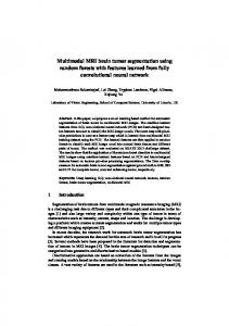
Fig. 1.1 Example of one of 40 patients in our high-grade glioma database, with tissues labeled as active cells (red), necrotic core (green), and edema (yellow). The figure shows a representative slice of the 3D image volumes.

edema (E) – as also do [2, 24]. Distinguishing between volumes of individual tissue types, especially active cells and necrotic core, is an important step for assessment of treatment response. For example, an effective drug might not change the gross tumor volume while still transforming active into necrotic cells. To detect this change, the volumes of both of these tissues must be monitored.

1.2.1 Motivation for using classification forests The efficiency of classification forests in dealing with high-dimensional spaces allows us to use non-local and context-aware features. These features span a much larger space than those considered by previous learning-based works on tumor segmentation, which use features which represent spatial points in the patient only very locally [2, 9, 18, 24, 25]. Context-aware features have two potential advantages. First, they enable the method to classify labels which cannot be distinguished in a lower-dimensional feature space. Second, our experiments suggest that learning based on context-aware features has an inherent regularizing effect on the results, which is enhanced in our approach through the additional use of initial probabilities. The inherent multi-label ability of classification forests is in contrast to most classifiers previously employed for tumor segmentation. Work which classifies multiple labels often uses SVMs [2, 24], which are inherently binary classifiers. In order to classify different tissues, they are applied hierarchically [2], or in the one-versus-all manner [24]. For these approaches, several classes have to be grouped together, and this step can make the distribution of the aggregate group more complex than the distribution of each individual class. For example, the intensity distribution of a tumor consisting of AC and NC tissues, which have very different representations in the multi-channel data (cf. Figure 1.1), is likely to be more complex than the distributions of the single classes. We circumvent this potential problem by classifying all tissues simultaneously, which requires us only to handle distributions of individual classes.

1 Segmentation of Brain Lesions from multi-channel MRI

5

Estimation of initial probabilities: T1-gad

T2

T1

FLAIR

DTI-q

posteriors based on tissue-specific GMMs in the intensity space GMM-B

GMM-AC

GMM-NC

GMM-E

DTI-p

(A) input data: MRI + DTI

pB

pAC

pNC

pE

(B) initial tissue probabilities

Classification Forest • spatially non-local, context-aware features • simultaneous multi-label classification

(C) segmentation

Fig. 1.2 Schematic Method Overview: Based on the input data (A), we first roughly estimate the initial probabilities for the single tissues (B), based on the local intensity information alone. In a second step, we combine the initial probabilities (B) with the input data from (A), resulting in a higher-dimensional multi-channel input for the classification forest. Through a simultaneous multi-label classification, based on non-local and context-aware features as well as initial tissue probabilities, the forest yields high-quality segmentation results (C).

1.2.2 Method: Classification forests with initial probabilities Our approach is based on classification forests as presented in Chapter ??. Previously, several works have applied discriminative learning techniques to tumor segmentation [2, 3, 7, 18, 24, 25]. Mostly, a learning method using comparably local features is combined with a regularization step, for example by modeling the boundary [8, 12], or by applying a variant of a random field spatial prior (MRF/CRF) [3, 7, 25]. The schematic overview of our approach is given in Figure 1.2. Besides using application-specific feature types to represent the input data, we adapt the standard classification forest by providing it with rough initial class probabilities as input, additionally to the raw input data. In its effect, this step is similar to the idea of auto-context from [23] and Chapter ??. In contrast to auto-context, we do not use the same type of classifier for the initial probabilities and the actual classification. Instead, for the estimation of initial probabilities, we use posterior probabilities based on intensity-based Gaussian Mixture models (GMM) for the single tissues. In comparison to computing the initial probabilities by classification forests, the GMMbased modeling has the advantage of a faster training, at the cost of a lower quality of the probability estimates (cf. Figure 1.5). We describe the estimation of the initial probabilities in Section 1.2.2.1. The advantage of an auto-context-type approach is that is has an applicationspecific regularizing effect, which is learned based on the input data. With such a regularization approach, we achieve high-quality results without using an explicit regularization model. This not only results in a more application-specific inherent

6

Geremia et al.

regularization, but due to the omission of an explicit regularization module, our approach has a low model complexity. Besides the use of initial tissues probabilities, the second important characteristic of our approach is that we use spatially non-local and context-aware features, with their advantages as discussed above. We describe the types of the the context-aware features that we use in Section 1.2.2.2. As described in the introduction, we classify the four classes C = {B, AC, NC, E} for background (B), active cells (AC), necrotic core (NC), and edema (E). Based on the tissue-specific segmentation results, we define the gross tumor as GT=AC∪NC. The MR data I = (IT1-gad , IT1 , IT2 , IFLAIR , IDTI-q , IDTI-p ) serves as input data, while the learning is based on expert voxel-wise manual annotations of the training data set.

1.2.2.1 Estimating initial probabilities As the first step of our approach, we estimate the initial class probabilities for a given patient as posterior probabilities based on the likelihoods obtained by training a set of GMMs on the training data. For each class c ∈ C, we train a single GMM, which captures the likelihood p(I|c) of the multi-dimensional intensity for this class. For a given testing data set I, the GMM-based posterior probability pcGMM for the class c is estimated for each point p∈R3 by pGMM (c|p) =

p(I(p)|c) pc , ∑c j p(I(p)|c j ) pc j

(1.1)

with pc denoting the prior probability for the class c, based on its relative frequency. We can now use the probabilities pcGMM (p)= pGMM (c|p) directly as input for the decision forests, in addition to the multi-channel MR data I. So now, our data for one patient becomes GMM GMM C=(IT1-gad , IT1 , IT2 , IFLAIR , IDTI-q , IDTI-p , pAC , pNC , pEGMM , pBGMM ) .

(1.2)

For simplicity, we will denote single channels by C j . Please note that we can use the GMM-based probabilities for maximum a posteriori classification by cˆ = arg maxc pGMM (c|p). We will use this for a base line comparison in Section 1.2.3.

1.2.2.2 Spatially non-local and context-aware feature types We employ three features types, which are intensity-based and parameterized. These features describe a point to be labeled based on its non-local neighborhood, which type makes them context-aware. We denote the parameterized feature types by xparams . During training, the type and parameters for the features are randomly drawn at evtype ery node. Every instantiated and selected feature xparams with its unique parameters

1 Segmentation of Brain Lesions from multi-channel MRI

7

Fig. 1.3 Examples of results on 8 patients. Obtained by a forest with GMM, MR, and DTI input, with training on 30 patients. The high accuracy of our results is quantitatively confirmed in Figs. 1.4 (AC=red, NC=green, E=yellow). Again, only representative slices of the 3D data set are shown.

corresponds to one dimension of the feature space F with dimension d 0 . Our feature space is much higher-dimensional than those used in previous work. We use the following notation: p is a spatial location to be assigned a class label, and C j is an input channel. Rl (p) denotes a p-centered and axis aligned 3D box region in C j with edge lengths l = (lx , ly , lz ), and u∈R3 is an offset vector. • Feature Type 1 - Intensity difference: This feature type measures the intensity difference between p in a channel C j1 and an offset point p + u in a channel C j2 probe

x j1 , j2 ,u (p,C) = C j1 (p) −C j2 (p + u) .

(1.3)

• Feature Type 2 - Mean intensity difference: This feature type measures the difference between intensity means of a box around p in C j1 , and a box around an offset point p + u in the (potentially different) channel C j2 xbox j1 , j2 ,l1 ,l2 ,u (p,C) =

1 1 ∑ C j1 (p0 ) − |Rl | 0 ∑ C j2 (p0 ) . |Rl1 | p0 ∈R 2 p ∈R (p+u) (p) l1

(1.4)

l2

• Feature Type 3 - Intensity range along ray: This feature type captures the intensity range along a 3D line between p and p+u in one channel. This type is designed with the intuition that structure changes can yield a large intensity change, e.g. NC being dark and AC bright in T1-gad. ray

x j,u (p,C) = max(C j (p + λ u)) − min(C j (p + λ u)) with λ ∈ [0, 1] . λ

λ

(1.5)

8

Geremia et al.

1.2.3 Evaluation We evaluate our approach on a set of multi-channel 3D MR data for 40 patients suffering from high-grade gliomas. All data is acquired prior to treatment on the same MR scanner. For all 40 patients, a manual segmentation of the three classes of AC, NC, and E is obtained in 3D with an interactive segmentation tool. We try to keep the amount of data pre-processing at a minimum. We perform skull stripping of MR channels [20], and for each patient we perform an affine intra-patient registration of all channels to the T1-gad image. We also avoid a full bias-field correction, and only align the mean intensities of the images within each channel by a global multiplicative factor. All these steps are fully automatic. The evaluation reports the Dice score between the manual segmentations and the results. Besides the the tissue-specific segmentation results, we also evaluate the segmentation quality for the gross tumor (GT) by defining it as GT=AC∪NC.

1.2.3.1 Experiments We perform an extensive series of cross-validation experiments to evaluate our method. For this, the 40 patients are randomly split into non-overlapping training and testing data sets. To investigate the influence of the size of the training set and generalization properties of our method, we perform experiments with following training/testing sizes: 10/30, 20/20, 30/10. For each of the three ratios, we perform 10 tests, by randomly generating 10 different training/testing splits. To demonstrate the influence of the single components of the method, we also perform tests on forests without GMMs, and compare to the results of GMM only. Finally, we investigate the influence of using DTI, by performing all experiments also with MR input only. Overall, this results in 30 random training sets, and 600 tests for each of the 6 approaches. The evaluation is performed with all images sampled to isotropic spatial resolution of 2mm, and forests with T =40 trees of depth D=20. With these settings, the training of one tree takes 10-25 min, and testing 2-3 min, depending on the size of training set and the number of channels. The algorithm and feature design were done on an independent 20/20-fold. Figure 1.3 shows a visual example of the results, while the quantitative evaluation and more details are given in Figure 1.4. We observe an improvement of the segmentation accuracy by the proposed method (Forest(GMM,MR,DTI)) compared to the other tested configurations. Comparison to quantitative results of other approaches is difficult for a number of reasons, most prominently the different input data. To provide some indicative context, we cite results of a recent work from [2]. There, the mean and standard deviation for a leave-one-out cross-validation on 10 glioma patients, based on multichannel MR are as follows: GT: 77±9, AC: 64±13, NC: 45±23, E: 60±16. Our results compare favorably. For our 30/10-tests we get: GT: 90±9, AC: 85±9, NC: 75±16, E: 80±18, and for the more challenging 10/30-tests (less training data), we get GT: 89±9, AC: 84±9, NC: 70±19, E: 72±23.

1 Segmentation of Brain Lesions from multi-channel MRI

DICE mean

100%

GMM(MR)

GMM(MR,DTI)

Forest (MR)

Forest (MR,DTI)

9 Forest (GMM,MR) Forest (GMM,MR,DTI)

90% 80% 70% Gross Tumor Active Cells Necrotic Core Edema

60% 50% 10/30 20/20 30/10

10/30 20/20 30/10

10/30 20/20 30/10

10/30 20/20 30/10

10/30 20/20 30/10

10/30 20/20 30/10

10/30 20/20 30/10

10/30 20/20 30/10

10/30 20/20 30/10

10/30 20/20 30/10

10/30 20/20 30/10

10/30 20/20 30/10

Std. dev.

30% 20% 10% 0%

Fig. 1.4 Average mean and standard deviations of DICE scores, for experiments on 10 random folds, with the training/testing data set sizes of 10/30, 20/20, and 30/10. From left to right, the approaches yield higher mean scores, with lower standard deviations. Our approach (rightmost) shows increased robustness to amount of training data, indicating better generalization. Gross Tumor

Active Cells

Necrotic Core

Edema

tree depth D

20 18

16 14 12 15 20 25 30 35 40 number of trees T

15 20 25 30 35 40 number of trees T

15 20 25 30 35 40 number of trees T

15 20 25 30 35 40 number of trees T

Fig. 1.5 Sensitivity to parameters is tested by varying the number of trees T = [15, 40] and the tree depth D = [12, 20]. The figure shows mean Dice scores for ten random 30/10-cross-validation tests. We observe robustness, in particular the number of trees.

Sensitivity to variation of parameters is tested by varying T ∈[15, 40] and D∈ [12, 20], for the ten 30/10-tests. The results are summarized in Figure 1.5. We observe robustness to the selection of these values, especially T .

10

Geremia et al.

1.3 Classification forests for segmentation of MS lesions In this section, we present the application of classification forests to the challenging task of segmentation of multiple sclerosis lesions.2 Multiple Sclerosis (MS) is a chronic, inflammatory and demyelinating disease that primarily affects the white matter of the central nervous system [11]. Automatic detection and segmentation of MS lesions can help diagnosis and patient follow-up. It offers an attractive alternative to manual segmentation which remains a timeconsuming task and suffers from intra- and inter-expert variability. However, MS lesions show a high variability in appearance and shape which makes automatic segmentation a challenging task. In particular, MS lesions lack common intensity and texture characteristics, their shapes are variable and their location within the white matter varies across patients. Our segmentation problem can be formalized as a binary classification of voxel samples into either background or lesions. Taking advantage of context-aware features in the classification task is key to detect the appearance differences of MS lesions with respect to healthy brain tissue. Subsequently, we use the classification forest technique for MS lesion segmentation. We exploit a specific discriminative symmetry feature which stems from the assumption that the healthy brain is approximately symmetric with respect to the mid-sagittal plane and that MS lesions tend to develop in asymmetric ways. We then show how the forest combines the most discriminative channels for the task of MS lesion segmentation.

1.3.1 Data The MICCAI 2008 Grand Challenge (MSGC) [22] makes publicly available two datasets through their website: a public dataset of labeled MR images which can be used to train a segmentation algorithm; and a private dataset of unlabeled cases on which the algorithm should be tested. The public dataset contains 20 cases which are labeled by a medical expert rater. The private dataset contains 25 cases, each annotated by three expert raters. For each case, 3 MR volumes are provided: a T1weighted image, a T2-weighted image and a FLAIR image. We sub-sample and crop the images so that they all have the same size, 159 × 207 × 79 voxels, and the same resolution, 1 × 1 × 2 mm3 . RF acquisition field inhomogeneities are corrected [15] and inter-subject intensity variations are normalized [17]. The images are then aligned on the mid-sagittal plane [16]. A spatial prior is added by registering the MNI atlas [4] to the anatomical images, each voxel of the atlas providing the probability of belonging to the white matter (PWM ), the grey matter (PGM ) and the cerebrospinal fluid (PCSF ). Please see also Figure 1.6. Both anatomical images and spatial priors will be treated under the unified term channel, and denoted C ∈ (IT1 , IT2 , IFLAIR , PWM , PGM , PCSF ). 2

More details can be found in [5].

1 Segmentation of Brain Lesions from multi-channel MRI IT1

IT2

IFLAIR

11 GT

PWM

Fig. 1.6 Sample case from the public Grand Challenge dataset. From left to right: preprocessed T1-weighted (IT1 ), T2-weighted (IT2 ) and FLAIR MR images (IFLAIR ), the associated ground truth GT and the registered white matter atlas (PWM ).

1.3.2 Feature types For the segmentation of MS lesions, we compute three types of intensity-based features. The actual feature types differ from the ones used for brain tumors in Section 1.2.2.2 in order to match the specifics of the MS lesion segmentation. However, it is interesting to note that the feature types for both tasks are similar in nature, and most importantly, both use the idea of spatial context-awareness. Of the following feature types, the first one is local, measuring only the local intensity in one single channel, while the other two are non-local and context-aware. • Feature type 1 - Local intensity: This local feature type measures the intensity in channel C at the location p, where C is either an MR image, or a prior channel xloc j (p) = C j (p) .

(1.6)

• Feature type 2 - Context-rich: This non-local feature type compares the intensity at the voxel of interest p with mean intensities of distant regions, in possibly different channels. More specifically, it compares the local voxel value in channel C1 with the mean value in channel C2 over two 3D boxes R1 and R2 within an extended neighborhood. Here, Ri stands for Rli (p + ui ), that is, a box with side lengths li , centered around an offset point p + ui . The feature type thus reads xcont j1 , j2 ,R1 ,R2 (p) = C j1 (p) −

1 1 C j2 (p0 ) − C j2 (p0 ) , ∑ |R1 | p0 ∈R |R2 | p0∑ ∈R 1

(1.7)

2

where C1 and C2 can be both, intensity or prior channels. The regions R1 and R2 are sampled randomly in a large neighborhood of the voxel v (cf. Figure 1.7). The sum over these regions is efficiently computed using integral volume processing [19]. • Feature type 3 - Symmetry: The second context-aware feature compares the voxel of interest at p with its symmetric counterpart with respect to the mid-

12

Geremia et al.

𝑅1 (b)

𝑆(𝑝)

𝑝

(f)

𝑅2

(g) (c)

(a)

(d)

(h)

(e)

(i)

Fig. 1.7 2D illustration of contextaware features. (a) A context-rich feature with two regions R1 and R2 (blue boxes) offset relatively to p (small red square). (b-d) Three examples of randomly sampled features in an extended neighborhood. (e) The symmetric feature with respect to the mid-sagittal plane. (f) The hard symmetric constraint. (g-i) The soft symmetry feature considering neighboring voxels in a sphere of increasing radius.

sagittal plane, noted S(p) sym

x j (p) = C j (p) −C j ◦ S(p) ,

(1.8)

where C j is restricted to be an intensity channel. Instead of comparing with the exact symmetric S(p) of the voxel, we consider, respectively, its 6, 26 and 32 neighbors in a sphere S (cf. Figure 1.7), centered on S(p). We obtain a softer version of the symmetric feature which which loosens the hard symmetric constrain and reads sym

{C(p) −C(p0 )} . xC,S (p) = min 0 p ∈S

(1.9)

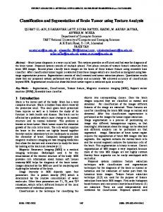
1.3.3 Experiments We train a classification forest on the whole public dataset from the MS Lesion Challenge, i.e. 20 labeled cases. Forest parameters are fixed to the following values: number of random regions |T | ' 950, number of trees T = 30, tree depth D = 20, lower bound for the information gain Imin = 10−5 , and the posterior threshold τposterior = 0.5. Considerations that lead to these parameter values are detailed in Section 1.3.4.2. The MSCG website carried out a complementary and independent evaluation of our algorithm on the previously unseen private dataset. The results, reported in Table 1.1, confirm a significant improvement over [21] which won won the MICCAI MS Segmentation Challenge 2008. The presented approach achieves, on average, a slightly higher true positive rate (TPR), which is beneficial, and a comparable false positive rate (FPR), but with lower volume difference (VD) and surface distance (SD) values (see Table 1.1). Pair-sample p-values were computed for the t-test on the private dataset. Results show significant improvement over the method presented in [21] on SD, p = 4.2 · 10−6 and p = 6.1 · 10−3 for CHB and UNC raters respectively.

1 Segmentation of Brain Lesions from multi-channel MRI Rater Metric [%] Souplet et al. [21] VD 86.48 ± 104.9 SD 8.20 ± 10.89 CHB TPR 57.45 ± 23.22 FPR 68.97 ± 19.38 VD 55.76 ± 31.81 SD 7.4 ± 8.28 UNC TPR 49.34 ± 15.77 FPR 76.18 ± 17.07

Class. Forest 52.94 ± 28.63 5.27 ± 9.54 58.08 ± 20.03 70.01 ± 16.32 50.56 ± 41.41 5.6 ± 6.67 51.35 ± 19.98 76.81 ± 11.70

13 RI [%] p-value −38.7 0.094 −35.7 4.2 · 10−6 +1.0 0.90 +1.5 0.70 −9.4 0.66 −24.3 6.1 · 10−3 +3.9 0.54 +0.1 0.83

Table 1.1 Average results computed by the MSGC on the private dataset and compared to the method presented in [21]. The relative mean improvement over the algorithm from [21] on the private dataset is defined as RI = (scoreRF − scoreSouplet )/scoreSouplet , as well as the p-value. The independent quantitative evaluation confirms an improvement over [21], with significant improvements in boldface. Our approach achieves a slightly higher true positive rate (TPR) and a comparable false positive rate (FPR), but with much lower volume difference (VD) and surface distance (SD) values.

1.3.4 Discussion 1.3.4.1 Interpretation of segmentation results Although segmentation results include most MS lesions delineated by the expert (see Figure 1.8), we observe that some MS lesions are missing. Missed MS lesions are located in specific locations which are not represented in the training data, e.g. in the corpus callosum (see Figure 1.8, slice 38). This is a limitation of the supervised approach. In this very case, however, the posterior map highlights the missed lesion in the corpus callosum as belonging to the lesion class with high uncertainty. Low confidence (or high uncertainty) reflects the incorrect spatial prior inferred from an incomplete training set. Indeed, in the training set, there are no examples of MS lesions appearing in the corpus callosum. On the contrary, the classification forest is able to detect suspicious regions with high certainty. Suspicious regions are visually very similar to MS lesions and widely represented in the training data, but they are not delineated by the expert, e.g. the left frontal lobe lesion again in Figure 1.8, slice 38. The appearance model and spatial prior implicitly learned from the training data points out that hyper-intense regions in the FLAIR MR sequence which lie in the white matter can be considered as MS lesions with high confidence.

1.3.4.2 Influence of forest parameters This section aims at understanding the effect of the number of trees T and their depth D on the quality of segmentation results. A 3-fold cross-validation on the public dataset is carried out for each parameter combination. Segmentation results are evaluated for each combination using two different metrics: the area under the receiver operating characteristic (ROC) curve

14

Geremia et al. IFLAIR and GT

Posterior Plesion

IFLAIR and Seg

axial slice 42

axial slice 38

IT1 and GT

Fig. 1.8 Segmenting Case CHB05 from the public MSGC dataset. From left to right: preprocessed T1-weighted (IT1 ), T2-weighted (IT2 ) and FLAIR MR images (IFLAIR ) overlayed with the associated ground truth GT, the posterior map Plesion displayed using an inverted grey scale and the FLAIR sequence overlayed with the segmentation Seg = (Plesion > τposterior ) with τposterior = 0.5. Segmentation results show that most of lesions are detected. Although some lesions are not detected, e.g. a lesion in the corpus calossum in slice 38, they appear enhanced in the posterior map. Moreover the segmentations of slices 38 and 42 show peri-ventricular regions, visually very similar to MS lesions, but not delineated in the ground truth.

and the area under the precision-recall curve. The ROC curve plots the true positive rate (TPR) vs. the false positive rate (FPR) scores computed on the test data for every value of τposterior ∈ [0, 1]. The precision-recall curve plots the positive predictive value (PPV) vs. TPR scores computed on the test data for every value of τposterior ∈ [0, 1].3 The results are reported in Figure 1.9. This analysis was carried out a posteriori using out-of-bag samples. We observe that 1) for a fixed depth, increasing the number of trees leads to better generalization; 2) for a fixed number of trees, low depth values lead to underfitting while high depth values lead to overfitting; 3) overfitting is reduced by increasing the number of trees. Forest parameters were selected in a safety-area with respect to under- and overfitting. The safety-area corresponds to a sufficiently flat region in the evolution of the areas under the ROC and precision-recall curves. We also observe that the performance of the classifier stabilizes for sufficiently large forests. 3

With TP, FP, TN, and FN denoting the number of true/false positive/negatives respectively, we have TPR= TP/(TP + FN), FPR= FP/(FP + TN), and PPV= TP/(TP + FP).

1 Segmentation of Brain Lesions from multi-channel MRI

15

Fig. 1.9 Influence of forest parameters on segmentation results. Both curves were plotted using mean results from a 3-fold cross validation on the public dataset. Left: the figure shows the influence of forest parameters on the area under the precision-recall curve. Right: the figure shows the influence of forest parameters on the area under the ROC curve. The ideal classifier would ensure area under the curve to be equal to 1 for both curves. We observe that 1) for a fixed depth, increasing the number of trees leads to better generalization; 2) for a fixed number of trees, low depth values lead to underfitting while high values lead to overfitting; 3) overfitting is reduced by increasing the number of trees.

1.3.4.3 Analysis of the relevance of feature types and channels Unlike other classifiers, classification forests provide an elegant way of ranking the employed features according to their discriminative power. In this section, we aim at better understanding which are the most discriminative feature types (local, contextrich or symmetric) and input channels for the task of MS lesion segmentation. As a first step of the analysis, we compute the statistics of how often the single feature types are selected, without taking into account the depth at which the features are chosen. We observe that local features were selected in 24% of the nodes, context-rich features were selected in 71% of the nodes whereas symmetry features were selected in 5% of the nodes. In the second step of the analysis, we focus on the depth at which a given feature was selected. We find that for every tree in the forest, the root node always applies a local test on the FLAIR sequence. This means that out of all available features types, loc with all randomly drawn parameters, xFLAIR was found to be the most discriminacont tive. At the second level of the tree, a context-rich feature on spatial priors (xWM,GM ) appears to be the most discriminative over all trees in the forest. The major effect of this feature is to discard all voxels which do not belong to the white matter. The optimal decision sequence found while training the forest can thus be thought of as a threshold on the FLAIR MR sequence followed by an intersection with the white matter mask. Interestingly, this sequence matches the first and second step of the pipeline proposed by the winner method of the MICCAI 2008 challenge [21]. Note that in our case, this sequence is automatically generated by the forest during the training process.

16

Geremia et al.

1.4 Chapter Summary and Discussion In this chapter, we have demonstrated the power of classification forests when applied to the difficult tasks of segmenting high-grade brain tumors and MS lesions. We show how classification forests can be adapted to medical image analysis settings, such that they achieve high-quality results. Furthermore, we analyze of the influence of the forest parameters, and present an investigation of the importance of the single features and input channels. Classification forests allow us to use non-local and context-aware features, to perform simultaneous classification of the individual tissues, and to generalize well to unseen data, even with only a relatively small training set. We leverage these advantageous properties of classification forests to achieve highly accurate results in both applications. For the segmentation of brain tumors, we use classification forests as a fundamental building block and augment it by integrating the initial test-specific probabilities for the single tissues. Since our approach has an inherent regularizing effect, which is data and application based, we can omit an explicit regularization module, which results in a system with a comparably low model complexity. For the segmentation of MS lesions, we employ three types of features based on multi-channel intensity, and tissue priors. These features result in a context-aware classification forest, which improves the results on one of the state of the art algorithms on the public MS challenge dataset. Regarding the input channels, in the MS lesion example, we employ prior tissue probabilities as input, additionally to the specific patient test data. In the tumor segmentation example, we have seen that using tissue-specific initial probabilities as additional input can have a beneficial and regularizing effect. The choice of feature types depends heavily on the application. However, this step can be decoupled from the core forest functionality which makes the approach very flexible. While the particular choice of the feature types varies in our two examples, the chosen intensity-based features are similar in nature. They are intensity-based and efficient to compute, and demonstrate convincingly the potential of context-aware features in medical image analysis applications.

References

1. G. H. Barnett, editor. High-Grade Gliomas. Springer, 2007. 2. S. Bauer, L.-P. Nolte, and M. Reyes. Fully automatic segmentation of brain tumor images using support vector machine classification in combination with hierarchical conditional random field regularization. In Gabor Fichtinger, Anne Martel, and Terry Peters, editors, Proc. Medical Image Computing and Computer Assisted Intervention (MICCAI), volume 6893 of LNCS, pages 354–361. Springer Berlin / Heidelberg, 2011. 3. J. J. Corso, E. Sharon, S. Dube, S. El-saden, U. Sinha, and A. Yuille. Efficient multilevel brain tumor segmentation with integrated bayesian model classification. Trans. Medical Imaging (TMI), 27(5), 2008. 4. A. C. Evans, D. L. Collins, S. R. Mills, E. D. Brown, R. L. Kelly, and T. M. Peters. 3D statistical neuroanatomical models from 305 MRI volumes. In IEEE-Nuclear Science Symposium and Medical Imaging Conference, pages 1813–1817, 1993. 5. E. Geremia, O. Clatz, B. H. Menze, E. Konukoglu, A. Criminisi, and N. Ayache. Spatial decision forests for MS lesion segmentation in multi-channel magnetic resonance. Neuroimage, 2011. 6. A. Gooya, K. M. Pohl, M. Bilello, G. Biros, and C. Davatzikos. Joint segmentation and deformable registration of brain scans guided by a tumor growth model. In Proc. Medical Image Computing and Computer Assisted Intervention (MICCAI), 2011. 7. L. Gorlitz, B. H. Menze, M.-A. Weber, B. M. Kelm, and F. A. Hamprecht. Semi-supervised tumor detection in magnetic resonance spectroscopic images using discriminative random fields. In Proc. of DAGM, 2007. 8. S. Ho, E. Bullitt, and G. Gerig. Level-set evolution with region competition: automatic 3-D segmentation of brain tumors. In Proc. Int. Conf. on Pattern Recognition (ICPR), 2002. 9. C.H. Lee, S. Wang, A. Murtha, M. Brown, and R. Greiner. Segmenting brain tumors using pseudo-conditional random fields. In MICCAI, 2008. 10. B. H. Menze, K. V. Leemput, D. Lashkari, M.-A. Weber, N. Ayache, and P. Golland. A generative model for brain tumor segmentation in multi-modal images. In Proc. Medical Image Computing and Computer Assisted Intervention (MICCAI), 2010. 11. Calabresi P. Multiple sclerosis and demyelinating conditions of the central nervous system. In Cecil Medicine. Saunders Elsevier, 2007. 12. K. Popuri, D. Cobzas, A. Murtha, and M. J¨agersand. 3D variational brain tumor segmentation using dirichlet priors on a clustered feature set. International Journal of Computer Assisted Radiology and Surgery, 2011. 13. M. Prastawa, E. Bullitt, S. Ho, and G. Gerig. A brain tumor segmentation framework based on outlier detection. Medical Image Analysis (MedIA), 2004. 14. S. J. Price, A. Pe˜na, N. G. Burnet, R. Jena, H. A. L. Green, T. A. Carpenter, J. D. Pickard, and J. H. Gillard. Tissue signature characterisation of diffusion tensor abnormalities in cerebral gliomas. European Radiology, 14:1909–1917, 2004. 10.1007/s00330-004-2381-6.

17

18

References

15. S. Prima, N. Ayache, T. Barrick, and N. Roberts. Maximum likelihood estimation of the bias field in MR brain images: Investigating different modelings of the imaging process. In Proc. Medical Image Computing and Computer Assisted Intervention (MICCAI), LNCS 2208, pages 811–819. Springer, 2001. 16. S. Prima, S. Ourselin, and N. Ayache. Computation of the mid-sagittal plane in 3D brain images. Trans. Medical Imaging (TMI), 21(2):122–138, 2002. 17. D. Rey. D´etection et quantification de processus e´ volutifs dans des images m´edicales tridimensionnelles : application a` la scl´erose en plaques. Th`ese de sciences, Universit´e de Nice Sophia-Antipolis, October 2002. (in French). 18. M. Schmidt, I. Levner, R. Greiner, A. Murtha, and A. Bistriz. Segmenting brain tumors using alignment-based features. In ICMLA, 2005. 19. J. Shotton, J. M. Winn, C. Rother, and A. Criminisi. TextonBoost for image understanding: Multi-class object recognition and segmentation by jointly modeling texture, layout, and context. Int. Journal on Computer Vision (IJCV), 81(1), 2009. 20. S. M. Smith. Fast robust automated brain extraction. Human Brain Mapping, 2002. 21. J.-C. Souplet, C. Lebrun, N. Ayache, and G. Malandain. An automatic segmentation of T2FLAIR multiple sclerosis lesions. In The MIDAS Journal - MS Lesion Segmentation (MICCAI 2008 Workshop), 2008. 22. M. Styner, J. Lee, B. Chin, M. S. Chin, O. Commowick, H. Tran, S. Markovic-Plese, V. Jewells, and S. K. Warfield. 3D segmentation in the clinic: A grand challenge II: MS lesion segmentation. In MIDAS Journal, pages 1–5, Sep 2008. 23. Z. Tu and X. Bai. Auto-context and its application to high-level vision tasks and 3D brain image segmentation. IEEE Trans. on Pattern Analysis and Machine Intelligence (PAMI), 32(10):1744–1757, 2010. 24. R. Verma, E. I. Zacharaki, Y. Ou, H. Cai, S. Chawla, A.-K. Lee, E.R. Melhem, R. Wolf, and C. Davatzikos. Multi-parametric tissue characterization of brain neoplasm and their recurrence using pattern classification of MR images. Academic Radiology, 15(8):966–977, 2008. 25. M. Wels, G. Carneiro, A. Aplas, M. Huber, D. Comaniciu, and J. Hornegger. A discriminative model-constrained graph-cuts approach to fully automated pediatric brain tumor segmentation in 3D MRI. In Proc. Medical Image Computing and Computer Assisted Intervention (MICCAI), 2008. 26. P. Y. Wen, D. R. Macdonald, D. A. Reardon, A. G. Cloughesy, T. F.and Sorensen, E. Galanis, J. Degroot, W. Wick, M. R. Gilbert, A. B. Lassman, C. Tsien, T. Mikkelsen, E. T. Wong, M. C. Chamberlain, R. Stupp, K. R. Lamborn, M. A. Vogelbaum, M. J. van den Bent, and S. M. Chang. Updated response assessment criteria for high-grade gliomas: response assessment in neuro-oncology working group. Am. J. Neuroradiol., 2010. 27. D. Zikic, B. Glocker, E. Konukoglu, A. Criminisi, C. Demiralp, J. Shotton, O. M. Thomas, T. Das, R. Jena, and Price S. J. Decision forests for tissue-specific segmentation of high-grade gliomas in multi-channel mr. In Proc. Medical Image Computing and Computer Assisted Intervention (MICCAI), 2012.