Supervised Brain Segmentation and Classification in Diagnostic of ...

Supervised Brain Segmentation and Classification in Diagnostic of Attention-Deficit/Hyperactivity Disorder Laura Igual1,2 (Invited Speaker)

Joan Carles Soliva3,4 Antonio Hern´andez-Vela1,2 Oscar Vilarroya3,4 Petia Radeva1,2

Sergio Escalera1,2

1

Department of Applied Mathematics and Analysis, Universitat de Barcelona, Spain Computer Vision Center of Barcelona, Universitat Aut`onoma de Barcelona, Spain Unitat de Recerca en Neuroci`encia Cognitiva, Department of Psychiatry, Universitat Aut`onoma de Barcelona, Spain 4 Hospital del Mar Research Institute (IMIM), Spain 2

3

INVITED PAPER

Abstract This paper presents an automatic method for external and internal segmentation of the caudate nucleus in Magnetic Resonance Images (MRI) based on statistical and structural machine learning approaches. This method is applied in Attention-Deficit/Hyperactivity Disorder (ADHD) diagnosis. The external segmentation method adapts the Graph Cut energy-minimization model to make it suitable for segmenting small, low-contrast structures, such as the caudate nucleus. In particular, new energy function data and boundary potentials are defined and a supervised energy term based on contextual brain structures is added. Furthermore, the internal segmentation method learns a classifier based on shape features of the Region of Interest (ROI) in MRI slices. The results show accurate external and internal caudate segmentation in a real data set and similar performance of ADHD diagnostic test to manual annotation. Keywords: Automatic Segmentation, Machine Learning, Graph Cut Framework, Brain Caudate Nucleus, ADHD Diagnostic

I. INTRODUCTION Significant effort has been put into automated segmentation of different structures in brain Magnetic Resonance Images (MRI) (see reviews [1], [2]). A good example of these efforts can be found in the Caudate Segmentation Evaluation challenge (CAUSE07) [3]. The most popular segmentation methods adopt the atlas-based approaches, which use data obtained from different subjects to construct a common anatomy for the brain image and apply it to further segmentations. However, the target object is not necessarily correctly represented by the atlas shapes. In this case, a more flexible and adaptive technique can be useful in order to ensure accurate segmentation results. In this sense, machine learning can be applied to learn useful information and improve segmentation approaches.

Figure 1.

Overview of the diagnostic test pipeline.

The approach applied in this paper combines the power of atlas-based segmentation with a new supervised energybased scheme based on the Graph Cut (GC) framework to obtain a globally optimal segmentation of the caudate structure in MRI [4]. GC theory has been used in many computer vision problems [5], such as binary segmentation [6], [7]. The original GC definition is limited to image information, and can fail when the brain structure in MRI is subtle and contrast is low. In order to overcome this problem, a variation of the classical GC model is defined adding supervised contextual

information. Previously-learned shape relations are exploited and moreover, boundary detection is reinforced using a new multi-scale edgeness measure. In [8], a manual strategy for internal caudate segmentation was proposed based on a simple geometric criterion. In this work, an automatic internal segmentation to separate caudate head and body parts is used based on learning a classifier based on shape features of the Region of Interest (ROI) [9]. Moreover, an automatic diagnostic test is evaluated, following the manual test proposed in [8]. Figure 1 shows the overview of the the diagnostic test method used in this paper. The obtained results by the fully-automatic method on real data are similar to the manual ones provided in [8]. The rest of the paper is organized as follows: Section II and Section III present the external and internal segmentation algorithms, respectively. Section IV reports and discuss the results of experiments on caudate nucleus segmentation, as well as ADHD diagnosis. Finally, Section V concludes the paper. II. E XTERNAL C AUDATE S EGMENTATION Graph-Cut Framework. Let us define X = (x1 , ..., xp , ..., x|P| ) as the set of pixels for a given grayscale image I; P = (1, ..., p, ..., |P|) as the set of indexes for I; N as the set of unordered pairs {p, q} of neighboring pixels of P under a 4-(8-) neighborhood system, and L = (L1 , ..., Lp , ..., L|P| ) as a binary vector whose components Lp specify assignments to pixels p ∈ P. Each Lp can be either ”foreground” or ”background”, or equivalently ”cau” or ”back” for our problem (abbreviations for caudate and background), indicating whether pixel p belongs to the caudate or background, respectively. Thus, the array L defines a segmentation of image I. The GC formulation defines the cost function E(L) which describes soft constraints imposed on boundary and region properties of L: E(L) = U (L) + δB(L),

(1)

where U (L) is the unary term (or region properties term), ∑ U (L) = Up (Lp ), p∈P

and B(L) is the boundary property term, ∑ B(L) = B{p,q} Ω(Lp , Lq ), {p,q}∈N

where,

{ 1, if Lp ̸= Lq Ω(Lp , Lq ) = 0, otherwise.

The goal of GC is to compute the global minimum of Eq. (1) from all segmentations L satisfying the hard constraints ∀p ∈ C, Lp = ”cau”, ∀p ∈ B, Lp = ”back”, where C ⊂ P, B ⊂ P, C ∩ B = ∅ denote the subsets of caudate and background seeds, respectively. Final segmentation is

computed over a defined graph using the min-cut algorithm to minimize E(L). Seed Initialization. In order to achieve a fully automatic method, the result of an atlas-based method, mainly based in [10] is used to define an initial segmentation. Caudate and background seeds are defined by performing morphological operations on the ROI obtained R0 in the atlas-based mask, as follows: caudate seeds, C = Erodeke (R0 ), where Erodeke denotes an erosion with a structural element of ke pixels; and background seeds, B = P \ Dilatekd (R0 ), where Dilatekd denotes a dilatation with a structural element of kd pixels. Unary Energy Term. The unary term is defined as the addition of two parts (unsupervised and supervised terms) as follows: Up (”cau”) = U Up (”cau”) + SUp (”cau”), Up (”back”) = U Up (”back”) + SUp (”back”). The unsupervised unary term is defined using caudate and background models based on graylevel information pertaining to the seeds. The unary potentials at each pixel p is initialized as: U Up (”cau”) = − ln(Pu (Lp = ”cau”)), U Up (”back”) = − ln(Pu (Lp = ”back”)). The probability Pu (Lp = ”cau”) is computed using the histogram of graylevels of caudate seeds and the probability Pu (Lp = ”back”) = 1 − Pu (Lp = ”cau”), since background seeds contain different tissues and it is difficult to extract a model directly from them. The unsupervised unary term estimates image-dependent caudate pixel probabilities based on caudate seeds. However, given the noisy information of MRI images and the small number of caudate seed pixels, a high generalization based on this term is not always guaranteed. In order to define the supervised unary term, a binary classifier is trained using a set of MRI slices as a training set. In particular, a pixel descriptor is extracted using a correlogram structure. The correlogram structure captures contextual intensity relations from circular bins around the pixel analyzed [11]. Given a pixel p, a correlogram Cc×r is defined, where c and r define the number of circles and radius of the structure. Then, each bin b from the set of n bins, with n = c · r, is defined as the area delimited by two consecutive circles of the given radius. Given the pixel p and its correlogram structure p Cc×r , its supervised caudate descriptor is defined as: dp = {∂1 , .., ∂k , .., ∂n·(n−1)/2 }, where ∂k is the signed substraction of graylevel information within a pair of bins in Cc×r . In this sense, the descriptor contains the n · (n − 1)/2 graylevel derivatives of all pairs of bins within Cc×r , which captures all spatial relations of graylevel intensities in the neighborhood of p.

The descriptors for a subset of pixels on C and B are extracted from the training set data. Given the set of descriptors, a linear SVM classifier is trained in order to predict caudate confidence on image pixels from new test data. In our case, the output confidence of the classifier is used as a measure of the ”probability” of a pixel belonging to the caudate. Then, the supervised unary potentials at each pixel p are: SUp (”cau”) = − ln(Ps (Lp = ”cau”)), SUp (”back”) = − ln(Ps (Lp = ”back”)). The probability of a pixel being marked as ”cau” is computed using the confidence of the SVM classifier over its correlogram descriptor Ps (Lp = ”cau”) = SVM(p). The probability of a pixel being marked as ”back” is computed as the negative of the output margin of the classifier Ps (Lp = ”back”) = −SVM(p). Boundary Energy Term. The boundary potential is defined as the following convex linear combination: B{p,q} = J(αN{p,q} + (1 − α)O{p,q} ). Terms N{p,q} and O{p,q} are defined using first and second intensity derivatives of the image to represent the intensity and geometric information, as follows: ( ) 1 (Ip − Iq )2 N{p,q} = exp − , ||xp − xq ||2 2σ 2 ( 2 ) θ{p,q} 1 O{p,q} = exp − . (2) ||xp − xq ||2 2β 2 The term θ{p,q} denotes the angle between two unitary vectors codifying the directions of minimum gradient variation in pixel p and q based on the Hessian eigenvectors. Moreover, given the high variability in contrast between the caudate and background in different parts of the images, the boundary term is weighted using an image-dependent multi-scale edgeness ∗ ). See [4] for more details. measure, J = (J1∗ , ..., Jp∗ , ..., J|P| Finally, by applying the min-cut algorithm over the defined energy function and image graph, the final caudate segmentation is obtained. III. I NTERNAL C AUDATE S EGMENTATION Given the external segmentation of the caudate nuclei in the MRI slices, the images corresponding to caudate head and body can be identified. Prior information of caudate shape in axial view of MRI volumes asserts that caudate head structure tends to be wider, while the body one tends to be elongate [12]. Moreover, first caudate slices in the axial projection of the MRI correspond to the head and the last ones to the body. An example of head and body caudate regions are shown in Figure 2. In order to perform the caudate head and body separation, the proposed method is based on the extraction of an extended set of caudate region features and the classification using

Figure 2. Example of caudate head image (left), and caudate body image (right), with caudate nuclei marked in red and green, respectively.

SVM. The set of features is composed by: ROI area, ratio between height and width of the ROI, height, width and area of the bounding box containing the ROI, extent (ratio of pixels in the ROI and pixels in the total bounding box), major and minor axis length of the ellipse that has the same normalized second central moments as the ROI, orientation of the ellipse, eccentricity (ratio of the distance between the foci of the ellipse and its major axis length), perimeters ratio (relation between the perimeter of the circle with the same area as the ROI, and the perimeter of the ROI), and x and y coordinates of the centroid. Once the set of features of the caudate regions are computed, SVM classifier is used to classify head and body caudate regions. In order to correct possible isolated misclassifications from SVM classifiers, contiguous slices are analyzed and postfiltered using the Decision Stump (DS) weak classifier. The DS technique is a machine learning model that consists of onelevel decision tree. A DS makes a polarity prediction based on the value of just a single input feature. DS is often used as a weak classifier in machine learning ensemble techniques. Here, DS is used to find a unique separation between caudate head and body areas. The procedure used is as follows, the error weight for each class is set to: ωe (Head) =

1 , #Head images

ωe (Body) =

1 . #Body images

A loss function describing the importance in the order of appearance of head and body images is defined for each case. The loss function Fx for head and body are linear and cubic to penalize the apparition of body regions in the first positions. Previous analysis says that 60% to 70% of the total of caudate slices belongs to caudate head. Once the weight and loss function are defined, the system searches for the optimal division between caudate head and body sections in terms of error, computing it as ωe · Fx . The position giving the smallest error will be selected as the separation position and the images will be consequently relabeled. After applying DS, most of the cases where there are images classified as head in the middle of a body section or vice versa disappear, and the global classification is, consequently, improved.

IV. E XPERIMENTS The experiments are devoted to evaluate the automatic external and internal caudate nucleus segmentation, as well as the ADHD diagnostic test.

2

1

0

A. Data and Validation Measures The study population includes 39 children with ADHD according to DSM-IV (referred from the Unit of Child Psychiatry at Hospital Vall Hebron in Barcelona) and 39 control subjects. Children with ADHD received a consensus diagnosis by an expert team (see [13] for a detailed explanation). For all subjects in the population MRI 1.5-T system volumes were used. MRI volumes were analyzed by its axial projection, which consists on 60 image planes with a resolution of 256 × 256 pixels. The volume of each voxel is 0.94 × 0.94 × 2 mm3 . Ground truth was build by means of an expert team as is described in [4] and [9].

−1

−2

−3

Relative absolute volume difference, in percent, VOLR − VOLG · 100, VD = VOLG where VOLR and VOLG correspond to the total volume of the R and G segmentations, respectively. Average symmetric surface distance, in millimeters, (N ) M ∑ ∑ d(BSi , BR )2 + d(BS , BRi )2 i=1 AD = i=1 , |BS | · |BR | where BS and BR correspond to the set of border voxels in R and G, respectively, and d(·, ·) returns the minimum Euclidean distance between two sets of voxels. Root Mean Square (RMS) symmetric surface distance, in millimeters, √ RMSD = AD. Maximum symmetric surface distance, in millimeters, ( ) MD = max d(BSi , BR ), d(BS , BRj ) . i,j

For evaluation of the internal segmentation, the following three validation measures based on True Positive (TP), False Positive (FP), True Negative (TN) and False Negative (FN) were computed: Sensitivity =

TP , TP + FN

SIE

VOE

VD

AD

RMSD

MD

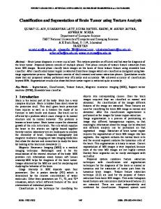
Figure 3. Quantitative results of AB and CaudateCut methods applied to URNC databases. Validation measures are, SIE: volumetric similarity index error (in %); VOE: volumetric overlap error (in %); VD: relative absolute volume difference (in %); AD: average symmetric surface distance (in mm); RMSD: root mean square symmetric surface distance (in mm); MD: maximum symmetric surface distance (in mm).

For evaluation of the external segmentation, different volumetric measures were considered: Volumetric similarity index (or mean overlap), in percent, R∩G · 100. SI = 2 R + G Volumetric union overlap, in percent, R ∩ G · 100. VO = R ∪ G

AB CaudateCut

Specificity = Accuracy =

TN , TN + FP

TP + TN . TP + TN + FP + FN

In this validation, 1039 caudate images from the 78 subjects were available, head corresponds to positive and body to negative. In the diagnostic test validation, ADHD patients corresponds to positive and control subjects to negative. B. Results The results are divided into three parts corresponding to a) the evaluation of the external segmentation method, denoted CaudateCut, and its comparison with an Atlas-based method (AB), b) the evaluation of the internal segmentation method, and c) the evaluation of the automatic ADHD diagnostic test, and its comparison with the manual test. External Segmentation. The performance of the CaudateCut, AMAS, and AB methods is compared. Figure 3 shows the results obtained in the experiments on both URNC and IBSR datasets for the six validation measures. SIE, VOE, and VD are measured in %, AD, RMSD, and MD are measured in mm, and all the measures are displayed in base 10 logarithm. For all validation measures, CaudateCut produced better results than both AB for URNC database. With regard to the volumetric measures, CaudateCut achieved good mean rates of 19.25% for SIE (equivalently, 80.75% SI), 31.98% for VOE (equivalently, 68.02% VO), and 16.22 for VD. Voxel by voxel mean measures are also acceptable, with 0.0024mm for AD, 0.0733mm for RMSD, and 35.70mm for MD. The large MD values are due to the recurrent errors present in the internal boundaries of the caudate defined between caudate head and body. It is important to note that CaudateCut showed robustness to AB results. Figure 4 shows qualitative CaudateCut

TABLE II S TATISTICAL ANALYSIS : MEAN OF THE RATIO R CBV/ B CBV AND STANDARD DEVIATION (σ) FOR CONTROL AND ADHD GROUPS , DIFFERENCE OF MEANS OF THE GROUPS , T- VALUE OF THE T- TEST ( WITH 0.05%), P - VALUE AND CONFIDENCE INTERVAL . Control ADHD

Mean 0.53 0.48

σ 0.06 0.05

Mean Diff.

t

p

0.05

2.4086

0.0092

TABLE III C OMPARISON OF MANUAL AND AUTOMATIC ADHD DIAGNOSTIC TEST. S ENSITIVITY, SPECIFICITY, A REA U NDER C URVE (AUC), AND O PTIMAL C UT-O FF VALUE (OCOV) ON THE TRAINING SET FOR MANUAL AND AUTOMATIC OF EXTERNAL AND INTERNAL SEGMENTATIONS . AUTO / AUTO STANDS FOR C AUDATE C UT AND SVM L INEAR +DS, RESPECTIVELY.

Figure 4. Example of CaudateCut results. GT is shown in green and CaudateCut segmentation in red.

results for the MRI slices of a control subject. In most of the slices, the CaudateCut segmentation result (red line) is highly comparable to the GT (green line). However, segmentation differences occur in the first and last caudate frames, where some voxels are classified as caudate by CaudateCut, but not by the GT (false positives). The inherent ambiguity of the caudate boundaries makes the expert’s task of manually defining the caudate start and end slices arduous. This introduces variability and produces errors in MRI atlas information corresponding to the end slices. It is difficult for CaudateCut to rectify this kind of error. The AB method introduces fake seeds in these positions and CaudateCut propagates these errors, since it can not remove the seeds. In the second column of the second row, some voxels are not classified as caudate, while they should be, according to GT (false negatives). This particular sample slice corresponds to the transition between caudate head and body, where the caudate shape changes abruptly from the rounded head to the elongated body [8]. Internal Segmentation. In order to evaluate the proposed methods we performed a leave-one-out validation strategy on the whole set of 1039 images. The performance of the method is shown in Table I, where the accuracy, sensitivity, and specificity of linear SVM with DS are shown. As it can be seen, results are accurate enought. ADHD Diagnostic Test. The objective of the diagnostic test is to discriminate between MRI volumes corresponding to ADHD and healthy subjects. In [8], authors present a diagnostic test to assist in the diagnosis of ADHD in children based on the ratio rCBV/bCBV. Using the Receiver Operating Characteristic (ROC) curve analysis on the defined ratio, the Optimal Cut-Off Value (OCOV) is estimated as the optimal raTABLE I R ESULTS OBTAINED FOR THE INTERNAL CAUDATE SEGMENTATION USING THE LEAVE - ONE - OUT VALIDATION STRATEGY. Accuracy 92.38%

Sensitivity 92.27%

Specificity 92.50%

Ext. seg./Int. seg. Manual/Manual [8] Manual/Manual Auto / Auto

Sensitivity 60% 55% 68.42%

Specificity 95% 85% 89.47%

AUC 0.84 0.73 0.75

OCOV 0.4818 0.483 0.491

tio for which the specificity is greater or equal than a threshold Thspec , which can be applied to classify new subjects. First, to analyze the significance of the ratio (rCBV/bCBV) in discriminating ADHD and control groups, we performed a Student’s t-test (with a threshold of p < 0.05). Table II summarizes the obtained statistics. In particular, mean ratio values, their standards deviation, the difference of means between the two groups and the results of the t-test are included. The result of the t-test was positive, confirming the statistical significance of the ratio measure. Second, in order to compare the proposed automatic strategy with the manual one we followed the validation steps indicated in [8]. In particular, we divided the set of 78 subjects in two subsets, one used for training and another for testing. We performed a ROC curve analysis using the training set to learn the OCOV as the optimal ratio threshold where the specificity was greater or equal than 85%. Table III shows the discriminative power of the system to differentiate between control and ADHD subjects. First row includes the results obtained in [8]. Second row correspond to the ”replica” of these results using the manual external and internal segmentation on the test set randomly defined by us. Finally, third row includes the results for the fully-automatic system, composed by the automatic external segmentation with CaudateCut and the automatic internal segmentation with linear SVM and DS. This fully-automatic system is giving results comparable with manual results, and can detect 68.42% of ADHD children correctly with only 11% of incorrect diagnostics on healthy subjects. Finally, we used a leave-one-out validation strategy on the set of 78 subjects to completely evaluate the proposed diagnostic test in the whole data set. In each test, we used ROC curve analysis to learn the OCOV as the optimal volume ratio threshold (specificity ≥ 85%). Table IV contains the mean sensitivity, specificity and OCOV of the leave-oneout validation. This fully-automatic system shows acceptable

TABLE IV R ESULTS OBTAINED FOR THE DIAGNOSTIC TEST USING LEAVE - ONE - OUT VALIDATION STRATEGY. Sensitivity 48.72%

Specificity 84.62%

THE

OCOV 0.4828

results to assist the diagnostic of ADHD. V. C ONCLUSION Inspired in a previously presented manual study stating that the ratio between rCBV and bCBV was statistically different in ADHD and control groups, we apply an automatic approach for external and internal caudate segmentation, followed by the brain classification in ADHD or control cases. The proposed external caudate segmentation combines the power of an atlas-based strategy and the adaptiveness of the defined energy function within the GC energy-minimization framework, in order to segment the small and low-contrast caudate structure. We defined the new energy function with data potentials by using intensity and geometry information, and also information of supervised learned local brain structures. Boundary potentials are also improved using a new multi-scale edgeness measure. The internal caudate segmentation classifies head and body regions based on shape features and a machine learning approach. The automatic segmentation method was completely validated on a datasets showing accurate performance. Finally, the automatic segmentation approach was applied in the ADHD diagnostic test, obtaining results comparable to manual test. Future lines of research include the use of multiplehypotheses for the GC initialization in order to increase the robustness to possible errors and the incorporation of 3D information in the caudate segmentation. From the clinical point of view, new features based on the caudate appearance can be added to analyze ADHD abnormalities in an automatic way. VI. Acknowledgements This work was supported in part by the projects: TIN200914404-C02, CONSOLIDER-INGENIO CSD 2007-00018, and MICINN SAF2009 -10901.

R EFERENCES [1] Balafar M, Ramli A, Saripan M, Mashohor S: Review of brain MRI image segmentation methods. Artificial Intelligence Review 2010, 33:261–274. [2] Duncan JS, Member S, Ayache N: Medical image analysis: progress over two decades and the challenges ahead. IEEE Transactions on Pattern Analysis and Machine Intelligence 2000, 22:85–106. [3] Ginneken BV, Heimann T, Styner M: 3D segmentation in the clinic: A grand challenge. In In: MICCAI Workshop on 3D Segmentation in the Clinic: A Grand Challenge. 2007. [4] Igual L, Soliva JC, Hernandez-Vela A, Escalera S, Jimenez X, Vilarroya O, Radeva P: A Fully-Automatic Caudate Nucleus Segmentation of Brain MRI: Application in Pediatric Attentiondeficit/Hyperactivity Disorder Volumetric Analysis BioMedical Engineering Online 2012. [5] Kolmogorov V, Zabih R: What energy functions can be minimized via graph cuts. PAMI 2004, 26:65–81. [6] Boykov Y, Funka-Lea G: Graph Cuts and Efficient N-D Image Segmentation. IJCV 2006, 70(2):109–131. [7] Boykov Y, Kolmogorov V: An Experimental Comparison of MinCut/Max-Flow Algorithms for Energy Minimization in Vision. IEEE Transactions on Pattern Analysis and Machine Intelligence 2001, 26:359–374. [8] Soliva JC, Fauquet J, Bielsa A, Rovira M, Carmona S, RamosQuiroga JA, Hilferty J, Bulbena A, Casas M, Vilarroya O: Quantitative MR analysis of caudate abnormalities in pediatric ADHD: Proposal for a diagnostic test. Psychiatry Research: Neuroimaging 2010, 182(3):238 – 243. [9] Igual L, Soliva JC, Gimeno AR, Escalera S, Vilarroya O, Radeva P: Automatic Internal Segmentation of Caudate Nucleus for Diagnosis of Attention-Deficit/Hyperactivity Disorder. In Proceedings of the International Conference on Image Analysis and Recognition, Lecture Notes in Computer Science, Springer-Verlag 2012. [10] Collins DL, Zijdenbos AP, Baar´e WFC, Evans AC: Animal+insect: Improved cortical structure segmentation. In IPMI, Springer 1999:210–223. [11] Escalera S, Forn´es A, Pujol O, Llad´os J, Radeva P: Circular Blurred Shape Model for Multiclass Symbol Recognition. IEEE Transactions on Systems, Man, and Cybernetics 2010. [12] Tremols V, Bielsa A, Soliva JC, Raheb C, Carmona S, Tomas J, Gispert JD, Rovira M, Fauquet J, Tobe˜na A, Bulbena A, Vilarroya O: Differential abnormalities of the head and body of the caudate nucleus in attention deficit-hyperactivity disorder. Psychiatry Res 2008, 163(3):270–8. [13] Carmona S, Vilarroya O, Bielsa A, Tr`emols V, Soliva JC, Rovira M, Tom`as J, Raheb C, Gispert J, Batlle S, Bulbena A: Global and regional gray matter reductions in ADHD: A voxel-based morphometric study. Neuroscience Letters 2005, 389(2):88–93.