We de ne the Grey Level Co-occurrence Function. (GLCF) g ; : 0;1;2;:::;n ?1]. 0;1;2;:::;n ?1] !Ras: g ;( ; ) = 1 ..... 21] A. Witkin, D. Terzopoulos and M. Kass, \Signal.
Draft Only 1
CLASSIFICATION IN SCALE-SPACE: APPLICATIONS TO TEXTURE ANALYSISy Paul Jackway�
In this paper we propose a technique for classifying images by modeling features extracted at di�erent scales. Speci cally, we use texture measures derived from Pap Smear cell nuclei images using a Grey Level Co-occurrence Matrix (GLCM). For a texture feature extracted from the GLCM at a number of distances we hypothesise that by modeling the feature as a continuous function of scale we can obtain information as to the shape of this function and hence improve its discriminatory power. This hypothesis is compared to the traditional method of selecting a given number of the best single distance measures. It is found, on the limited data set available, that the classi cation accuracy can be improved by modeling the texture features in this way. Index Terms | Multi-scale Approaches, Pattern Recognition, Texture Analysis.
1 Introduction
S
Brian Lovell�
Dept. of Electrical and Computer Engineering, University of Queensland, Brisbane 4072, AUSTRALIA This project is supported by the Cooperative Research Centre for Sensor Signal and Information Processing �
y
Andrew Bradley�
cale is of vital importance in the analysis and understanding of signals. The adage \You can't see the woods for the trees" is a classic example of a problem of scale. A forest can only be recognised as such within a particular range of distances (scales). If you are too close, the forest appears as a single branch, piece of bark or collection of molecules. From a distance of hundreds of kilometers the forest just becomes a small part of the shape and texture of the landscape. The idea that all the information in a signal is not contained at only one scale is of crucial importance. It has been shown that to fully analyse the structure of the signal it is necessary to relate information from a number of di�erent scales. A method of combining this information, proposed by Witkin [22], is to treat scale as a continuous variable rather than a parameter. Signal features measured at different scales can then be related if they lie on the same feature path in \scale-space". In the computer vision community, a variety of image structures have
been analysed at di�erent scales by using this multiscale representation [14]. A classic example of this scale-space analysis is in signal matching [21]. In this paper we have applied this same principle to the investigation of measures of image texture at varying scales. Most measures of texture being determined at a number of scales or distances [5,13]. We propose a method to incorporate the information from all these scales in a meaningful way, hence signi cantly reducing the dimensionality of the data, whilst maintaining as much useful information as possible.
2 Grey Level Co-occurrence Matrix Texture Measures
Grey Level Co-occurrence Matrix (GLCM) as T heproposed by Julesz [11] and later by Haralick et
al [7], has been shown to be a powerful technique for
measuring texture [1,6]. It is a second-order method that characterizes the probability that, given an image f : D � Z2 ! [0; 1; 2; : : :; n ? 1], the grey levels k = f (i; j ), and l = f (i0 ; j 0) co-occur. We de ne the distance between (i; j ) and (i0; j 0) as d = d ((i; j ); (i0; j 0)), which expressed in polar coordinates is r = jdj and � = 6 d. The GLCM is then Cr;� where each element c(k; l) is given by:
c(k; l) = Pr f (i0; j 0) = l j f (i; j ) = k : �
�
(1)
The GLCM, Cr;� , is constructed by rst quantising the image, f , into a \manageable" number of grey levels1 [0; 1; 2; : : :; n ? 1], and then, for every pixel (i; j ), examining the pixel (i0; j 0) for speci ed values of r and �. The GLCM, Cr;� , is then of size n � n, with entries, c(k; l), incremented every time the grey levels k and l co-occur. Probability estimates are obtained by dividing each entry in Cr;� by 1
In our case 16 [18].
the sum of all the entries. GLCM's are constructed at a number of distances, r, (scales) [1; 2; 3; : : :; m], and angles, �, [0� ; 45�; 90�; 135�] in the image. Note: the GLCM is constructed to be symmetric so that T Cr;� +Cr;� T Cr;� = , i.e., Cr;0� = Cr;180� Cr;T45� = 2 T Cr;225� , Cr;90� = Cr;270� , and Cr;T135� = Cr;315� . Once the GLCM, Cr;� , has been constructed, its \content" is characterized using descriptors that extract features from Cr;� . For example, a descriptor that has a relatively high value when the values of Cr;� are near the main diagonal, is the Inverse Difference Moment (Local Homogeneity):
IDMr;� =
XX
k
l
c(k; l) ; (1 + (k ? l)2)
(2)
while a descriptor such as Entropy measures randomness, reaching its highest value when the elements of Cr;� are equal:
Entr;� = ?
XX
k
l
c(k; l) ln c(k; l):
(3)
A number of other such features have been proposed [7,15], and are given for the continuous case in section 3. The conventional method of texture analysis using the GLCM is to treat these features, extracted at di�erent distances (scales), as independent features. Selecting a small subset of scales (often a single scale) that gives the highest discriminatory power [23]. We propose to treat these measurements of texture at each scale as sample points of a continuous function through scale-space. This function can then be reconstructed by interpolating the sample points of the functions extracted from the GLCM. This allows a whole new range of classical mathematical techniques for comparing functions to be used in the analysis and classi cation of textures.
3 Texture as a Function of Scale
Assume we have an image f : D � R2 ! [0; 1; 2; : : :; n ? 1], with the domain D bounded and of area ZZ A(D) = dxdy: (4) D
Since this image is de ned on a continuous domain, we need to reformulate the theory of Grey Level Co-occurrence Matrices (GLCM) for the continuous case. To unify our work with scale-space theory, we will use the notation � (scale) instead of r (distance) to denote pixel displacement.
Draft Only 2
We de ne the Grey Level Co-occurrence Function (GLCF) g�;� : [0; 1; 2; : : :; n ? 1] � [0; 1; 2; : : :; n ? 1] ! R as: g�;� (�; ) = A(1D) � ZZ � � I f (x; y) = �; f (x0; y 0) = dxdy; D (5) where, x0 = x + � cos �; (6) 0 y = y + � sin �; (7) and the indicator function, � � I f (x;�y) = �; f (x0; y 0) = 0 0 = 1 if (f (x; y ) = �) and (f (x ; y ) = ); 0 otherwise. (8) In other words, the GLCF estimates the probability that a pair of grey levels [�; ] will be found at a displacement [� cos �; � sin �] apart. Scale dependent texture features T (� ) are extracted by applying some functional to the GLCF. If this functional integrates g�� (�; ) over �; and �, then the texture feature of interest can be expressed as a function of scale. We write: T (�) = [g�;� (�; )] : (9) The following scale dependent functionals are continuous versions of commonly used [1,7,15] discrete textural feature measures: Energy:
En(�) =
Z ZZ
�
D
2 (�; ) d�d d� g�;�
(10)
Inverse Di�erence Moment (Local Homogeneity):
IDM (�) = Entropy:
Ent� = ? Correlation:
1 1 + ( � ? )2 g�;� (�; ) d�d d�: D (11)
Z ZZ
� Z ZZ
�
D
g�;� (�; ) ln g�;� (�; ) d�d d�: (12)
Corr� = Z ZZ
�
(� ? �� )( ? � )g�;� (�; ) d� d d�: �� � D (13)
Draft Only 3
1 ah(a) da; ?1
(14)
1 (a ? �)2 h(a) da: ?1
(15)
�= and variance:
�2 = Inertia:
In� =
Z ZZ
�
D
Z
Z
(� ? )2 g�;� (�; ) d�d d�
Cluster Shade:
3.1 Classi cation of Texture Functions
Z ZZ
Cs� =
�
(16)
D
((� ? �� ) + ( ? � ))3�
g�;� (�; ) d�d d�:
(17)
Cluster Prominence:
Cp� =
Z ZZ
�
D
((� ? �� ) + ( ? � ))4�
g�;� (�; ) d�d d�:
(18)
Note: Rotational invariance is obtained by integrating with respect to �, this can be done either before or after we integrate with respect to D. In the discrete case it is common [1,8] to average the GLCM matrices generated for each angle and then calculate the texture features from this one matrix. In a continuous version of this approach Energy would then be written as:
En� =
ZZ
Z
D �
as a continuous variable, and � to be calculated at angles other than 0�, 45�, 90�, and 135�. The number of samples needed to accurately t a function depends on the type of texture we are measuring. With the method we have chosen the nest resolution available is at a distance of one pixel, while the coarsest resolution would either be the largest distance in the image or the largest spatial texture of interest. These have been called the inner and outer scales [12], and are usually determined by the format of the original image.
g2
�;� (�; ) d�d�d :
We propose to use the actual shape of these scalespace texture functions to discriminate between different classes of images. In this way all of the available information is used to generate a model of the feature. The parameters of these models can then used as \high order" features in the classi cation scheme. This means that classi cation of new examples is done in parameter-space. An advantage of tting continuous functions is that we can also classify by integrating the area between the curves of a new example and the prototype normal and abnormal curves. We could then weight this area as a function of the variance (Mahalanobis distance) of the prototype curves, and then estimate the class of the new example as the class of the nearest prototype.
3.2 An Example 4
3
(19)
We have chosen to calculate the texture features for each angle and then average the feature values [18]. This reduces the averaging e�ect for features raised to powers greater than unity, e.g., equations 10, 17, and 18. This may be important if at one angle these texture features, have a much higher value than at all the other angles. Averaging with respect to � before calculating the function at that scale will reduce this e�ect. In this paper we approximate these scale dependent functionals by tting continuous functions to the discrete measurements extracted from the GLCM. However, we could have also tted a continuous function to the image, allowing direct calculation of the GLCF. This would also allow scale to be extracted
2
1 y(Scale)
where, mean:
0
−1
−2
−3
−4 0
2
4
6
8 Scale
10
12
14
16
Figure 1: Examples of two classes of line Purely for the purpose of illustration, we shall imagine that the functions of the form shown in gure 1 are measures of image texture at varying scale. Examples of one class being shown with solid lines while
examples from the other class are shown with dotted lines. 30 examples of each class were generated using y = mi x + ci + ", where " � N (� = 0; � 2 = 1), x = [1; 2; 3; : : :; 16], for one class mi = 0:1, ci = 0:8 and for the other mi = ?0:1, ci = ?0:8. There is a large amount of intraclass variation on these functions which makes discrimination at any one scale very di�cult. However, if a linear model is assumed and an equation of the form:
y = mx + c (20) is tted in a least mean squares sense to each example, we can then parameterize each example with only two features: the gradient m and the intercept c of the tted line.
Comparing gures 3 and 2 we can see that the samples are more clustered and separated in parameter-space rather than in the reduced distancespace. Therefore, improved classi cation accuracy would achieved using the model parameters rather than the two \best" scales. It should be noted that at least four scales are required to separate these two classes of functions with 100% accuracy on new, unseen data, and that, in this case, good (over 97%) classi cation accuracy would be achieved using only the gradient or the intercept parameters. In the above example, the two \best" scales were found using a branch and bound algorithm with the Bhattacharyya distance measure for determining feature separation [2,16].
4 Texture Analysis of Cervical Cell Nuclei
2.5 2 1.5
set was as detailed by Walker et al [18], T heanddataconsists of 61 segmented cell nuclei, there
1
Distance 14
Draft Only 4
0.5 0 −0.5 −1 −1.5 −2 −2.5 −3
−2
−1
0 Distance 2
1
2
3
Figure 2: Scatter plot for the two \best" scales Figure 2 shows a scatter plot for the 30 examples of each class, by selecting the two most discriminatory, or \best," scales. Figure 3 shows a scatter plot for the two parameters of the tted model, the gradient and the intercept.
being 30 normal and 31 abnormal cells. A classi cation accuracy of 96.7% has been reported for the best two features using a hyper-quadric decision surface, using three fold cross-validation2 [18]. The 7 features extracted from the GLCM were measured at distances 1 to 15 at odd intervals only, this gives a total of 8 distance measures. The \best" two features were selected using simultaneous forward selection of n, backward elimination of m, and were found to be Inertia and Inverse Distance Moment (IDM), both at a distance of 3. Normal Cell
Abnormal Cell
Normal Cell
Abnormal Cell
2 1.5 1
Intercept
0.5 0 −0.5 −1 −1.5 −2 −2.5 −0.25
−0.2
−0.15
−0.1
−0.05
0 0.05 Gradient
0.1
0.15
0.2
0.25
Figure 3: Scatter plot of the tted parameters
Figure 4: Examples of segmented normal and abnormal cervical cell nuclei Due to the di�erences in methodology this result should not be directly compared with the results shown in table 2. 2
Figure 4 shows examples of the texture in typical normal and abnormal cervical cell nuclei. It can be appreciated from this gure that it is rather di�cult for the untrained observer to distinguish between the two di�erent cell types. For the purpose of this study it was decided to rst classify the cells using only one of the 7 available texture features at a time, i.e., we would train and classify on just one (say, IDM) of the features at all the available distances. We compare classi cation accuracy for a model, with N parameters, tted to each texture feature, and for the best N distance measures (scales) for that feature. In this way it is possible to determine which method best extracts the useful information from the texture features. Then, we select the best N parameters from the best models tted to each texture feature and again classify the cervical cell data. This is compared to the conventional method of choosing N distances from all those available.
5 Results No. Features N Energy
1
2
3
4
N Scales N Parameters
70% 70% 70% 70% 68% 57% 53% 68%
N Scales
N Parameters
77% 85% 86% 85% 58% 77% 80% 90%
N Scales N Parameters
67% 83% 88% 88% 72% 75% 92% 85%
N Scales N Parameters
85% 81% 83% 81% 72% 75% 84% 70%
N Scales
N Parameters
90% 92% 91% 88% 84% 90% 90% 82%
N Scales N Parameters
70% 65% 63% 67% 54% 60% 73% 69%
IDM
Entropy
Correlation Inertia
Cluster Shade Cluster Prom
N Scales 62% 85% 81% 81% N Parameters 68% 72% 77% 90% Table 1: Comparison of classi cation accuracies for selecting the best N scales and tting a model with N Parameters Table 1 shows estimates of the true accuracy for each of the features selected and model tted. Polynomials have been tted so a 2 parameter model is a straight line, 3 parameters a quadratic and 4 a cu-
Draft Only 5
bic. A 1 parameter model in this case was chosen to be either the gradient or the intercept from the straight line model depending on which gave the highest discrimination. No. Features Best Scales Best Model
1 2 3 4 5 90% 92% 88% 87% 88% 83% 90% 94% 94% 94%
Table 2: Comparison of classi cation accuracies for the best N features Table 2 shows estimates of the true accuracy selecting N features from the original 56 distance measures3, and selecting N of the generated parameters from only the best model for each feature, i.e., from 21 parameter features. All features were rst normalised to be in the range [0,1] and then selected using a Sequential Forward Search with the Bhattacharyya distance measure for determining feature separation [2,16]. Note: The best two features were the same as used in [18]. Branch and bound analysis was not used because of its computational complexity when selecting 5 features from 56, it also gives no ranking of the features. The error estimate was obtained from a leaveone-out [19] random sub-sampling using K-Nearest Neighbours (with K=1). This strategy is computationally intensive, but is generally considered to be one of the most reliable estimators of true error rate.
6 Discussion
models to each of the 7 texture features F itting reduced the dimensionality of the original data
set from 56 to 21. This is a signi cant reduction in dimensionality and reduces the computational complexity of further feature selection. Karhunen-Lo�eve analysis has also been suggested for dimensionality reduction of texture features [17]. However, in initial trials we found the technique performed poorly in this case, and, so far, has not been investigated further. The classi cation accuracy was better for the tted models for 4 of the 7 texture features. This is despite the fact that the shapes of the texture functions are not that di�erent between normal and abnormal cells. This would indicate that even though the functionals used are perhaps not ideally suited, the technique still performs well. Figure 5 shows the shape of the texture function, Inertia, extracted from the cervical cell nuclei. For the 3
7 features each at 8 distances.
Draft Only 6
Inertia 25
20
15
10
5
0 0
5
10
15
Distance
Figure 5: Plots of the means and standard deviations of the Inertia texture measure for normal and abnormal cells normal cells the mean and standard deviations are shown by solid and dotted lines respectively, while for the abnormal cells, the mean and standard deviations are shown by dashed and dash-dotted lines respectively. In general the classi cation accuracy of each texture feature increased when we considered more than one scale. This con rms a result found by Conners and Harlow [1] and Weszka et al [20], and reiterates the fact that all the information in the signal is not contained at just one scale. The overall accuracy also increased when combining di�erent texture features together, a similar result was found by Gotlieb and Kreyszig for their atomic and composite classi ers [6]. When using all the texture features, the proposed technique did not perform as well as the conventional method for low dimensionality (2 and below), but did better when more features were added (dimensionality 3 and above). This is probably due to the fact that there is one distance of one texture feature4 that separates this data set well (with 90% accuracy). It is suspected that this will not be such a dominant feature on a larger data set. The highest classi cation accuracy of 94% was obtained using the proposed technique, and was found to be for 3, 4 or 5 parameters selected from the best texture feature models. However, if you consider that the di�erence between 92% and 94% accuracy on a data set of 61 examples is only 1 case, we infer that the results are comparable. It is hypothesised that the proposed method ex4
Inertia
at a distance of 3.
tracts the maximum amount of useful information from the features whilst signi cantly reducing their dimensionality. Higher order models will of course be able to t more complex scale-space functions, but at the expense of having a larger number of parameters and therefore increased dimensionality. If there is only one scale in the function that has any discriminatory power5, then this model based technique would probably not perform any better than the conventional method of picking this one \best" scale, though, this pathological worst case, is unlikely to appear very often in practice. If we used every distance measured for a feature and classi ed the data using distance measures weighted by the variance at each point, we would have included all of the available information. However, no reduction in dimensionality has been achieved and so a vast number of examples may be required to accurately separate the classes and give good performance on new, unseen, data. This problem is known as the \curse of dimensionality" [3] where an extremely large number of examples are required to accurately train the classi cation scheme. There may also be scales where there is no discriminatory power at all, and so including information from that scale in the analysis may well add noise and degrade performance. Scale should really be treated in a logarithmic manner, in this way changes in the texture function between, say scales 1 and 2 should be just as signi cant as changes in scale between 8 and 16. This was not done in this study as the data had already been collected at integer scales, but models should perhaps be tted to a logarithmic scale in future research. Another advantage of the model tting technique is that the features can be measured at as many distances or scales as you desire. The more samples of the continuous function the better, with the conventional method however, this would add to the dimensionality of the problem and make feature selection more computationally expensive. In this paper, only polynomial models have been discussed, there is of course a multitude of models and methods that could be used, such as autoregressive models, cubic splines, likelihood ratio tests etc. Classi cation in scale-space has only been applied to GLCM texture features in this paper, there are also a number of other scale dependent functionals that this technique can be applied to, Or, as in this case, one scale of one function that has a high (90%) level of discrimination. 5
Draft Only 7
e.g., features extracted from a morphological scale- [4] J. M. Gauch, \Multiscale image segmentation using
space [9], or a multi-scale gradient watershed regions [4,10].
7 Conclusions
W
[5] [6]
e have formulated a technique for classifying texture as a continuous function of scale. We have empirically shown the technique to perform as [7] well as (if not better than) the conventional method on textures derived from cervical cell nuclei. In addition, we have highlighted the following advantages of the proposed technique: [8]
� It uses information from a number of scales by
modeling the shape of the texture functions in [9] scale-space. � It reduces the dimensionality of the data, pro- [10] ducing \high order" features. � Dimensionality is not increased by taking more [11] distance measures. Caution should be used when drawing conclusions [12] from such a small data set, but the results are encouraging and provide a good foundation for further [13] research in this area.
8 Acknowledgements
[14]
he authors are grateful to P. Shield and G. Per- [15] T kins of the Royal Women's Hospital in Brisbane, for providing the slides and classifying the cell images used in this study. The software used for feature selection and K-Nearest Neighbour error estim- [16] ate was part of the tooldiag software package [16] and is based on material in Pattern Recognition: A Statistical Approach [2]. This project is supported by the Cooperative Research Centre for Sensor Sig- [17] nal and Information Processing.
9 References [1] R. W. Conners and C. A. Harlow, \A theoretical comparison of texture algorithms," IEEE Trans Pattern Anal Machine Intell, PAMI-2, no. 3, pp. 204{222, 1980. [2] P. A. Devijver and J. Kittler, in Pattern Recognition: A statistical approach. London: Prentice Hall, 1982. [3] R. O. Duda and P. E. Heart, in Pattern classi cation and scene analysis. New York: Wiley-interscience, 1973.
[18]
gradient watershed regions," University of Kansas, Lawrence, Unpublished report: Dept. Electrical Engineering and Computer Science, 1994. R. C. Gonzalez and R. E. Woods, Digital Image processing. Reading, Mass., Addison-Wesley, 1992. C. C. Gotlieb and H. E. Kreyszig, \Texture descriptors based on co-occurrence matrices," Computer Vision, Graphics, and Image Processing, 51, pp. 70{86, 1990. R. M. Haralick, K. S. Shanmugham and I. Dinstein, \Texture features for image classi cation," IEEE Trans Syst Man Cybern, SMC-3, no. 6, pp. 610{621, 1973. R. M. Haralick, \Statistical and structural approaches to texture," in Proceedings of the IEEE, vol. 67, no. 5. pp. 786{804, 1979. P. T. Jackway, \Morphological scale-space," in Proceedings 11th IAPR International Conference on Pattern Recognition. pp. 252{255, 1992. P. T. Jackway, \Morphological multiscale gradient watershed image analysis," in Proceedings of SCIA95 9th Scandinavian Conference on Image Analysis. 1995. B. Julesz, \visual pattern discrimination," IRE Transactions on Information Theory, Vol IT 8, pp. 84{92, 1962. J. J. Koenderink, \The Structure of Images," Biological Cybernetics, vol 50, pp. 363{370, 1984. M. D. Levine, Vision in man and machine. New York, McGraw-Hill, 1985. T. Lindeberg, \Scale-space theory: A basic tool for analysing structures at di�erent scales," Journal of applied statistics, Vol 21 , no. 2, pp. 225{270, 1994. S. H. Peckinpaugh, \An improved method for computing gray-level cooccurrence matrix based texture measures," Graphical models and image processing, Vol 53, no. 6, pp. 574{580, 1991. T. W. Rauber, M. M. Barata and A. S. Steiger-Garcao, \A Toolbox for the analysis and visualisation of sensor data in supervision," Universidade Nova de Lisboa, Portugal, Intelligent Robots group Technical report, 1993. J. T. Tou and Y. S. Chang, \Picture understanding by machine via textural feature extraction," in Proceedings of IEEE conference on Pattern Recognition and image processing. pp. 392{399, 1977. R. Walker, P. Jackway, B. Lovell and D. Longsta�, \Classi cation of cervical cell nuclei using morphological segmentation and textural feature extraction," in Proceedings of the 2nd Australian and New Zealand Conference on Intelligent Information Systems. pp. 297{301, 1994.
[19] S. M. Weiss and I. Kapouleas, \An empirical comparison of pattern recognition, neural nets, and machine learning classi cation methods," in Proceedings of the eleventh international joint conference on arti cial intelligence. San Mateo: Morgan Kaufmann, pp. 781{ 787, 1990. [20] J. S. Weszka, C. R. Dyer and A. Rosenfeld, \A comparative study of texture measure for terrain classi cation," IEEE Trans Syst Man Cybern, SMC-6, no. 4, pp. 269{285, 1976. [21] A. Witkin, D. Terzopoulos and M. Kass, \Signal Matching through Scale-space," The International Journal of Computer Vision, pp. 133{144, 1987. [22] A. P. Witkin, \Scale-space ltering," in Proceedings of the International Joint Conference on Arti cial Intelligence. Palo Alto: Kaufman, pp. 1019{1022, 1983. [23] S. W. Zucker and D. Terzopoulos, \Finding structure in co-occurance matrices for texture analysis," Computer graphics and image processing, Vol 12, pp. 286{ 308, 1980.
Draft Only 8