the entire population. From each sub-population we calcu- late a test statistic which can be used to construct a single hypothesis test. To control the global type-1 ...
Classification of Non-Stationary Random Signals using Multiple Hypotheses Testing Geoff Roberts and Boualem Boashash Signal Processing Research Centre QUT GPO Box 2434 Brisbane Q. 4001 Australia ga.roberts @ qut .edu.au
Abstract
we introduce a time-varying quadratic discriminantfunction using the spectrogram. We apply the generalised sequentially rejective Bonferroni test to the multiple hypotheses that can be constructed at different points in time from this discriminant function. Other classification techniques have been suggested recently using time-frequency distributions (TFD). In [8] the authors extended the log-spectral distance to the timefrequency case and in [3] the authors proposed a technique based on the cross Wigner-Ville distribution. In the sequel we will discuss how our method deviates from the existing solutions.
In this paper we introduce a new time-jrequency based method for classifying non-stationary random signals. The method involves dividing the signal into overlapping or nonoverlapping segments considered to be subpopulations of the entire population. From each sub-population we calculate a test statistic which can be used to construct a single hypothesis test. To control the global type-1 error it is necessary to consider the hypotheses from all subpopulations simultaneously. We use the generalised sequentially rejective Bonferroni multiple hypothesis test which provides an eficient method to simultaneously test multiple hypotheses while maintaining the global type-1 errox Finally, we show the results of classifying time-dependeniAR(1) processes which have identical expected instantaneous power and power spectral densities but direrent time-frequency representations.
2. Time-frequency discrimination In this paper we developed the theory for the simplest case of classifying the signal into one of two classes. It is straightforwardto extend the results for a larger number of classes. To classify a signal into one of two classes we formulate the test
1. Introduction The problem of signal classification can be divided into three consecutive sub-problems: detection of the presence of a signal; segmentation to determine the time interval of the signal; and classification of the signal into one of a finite number of classes. In this work we will focus on classifying an observation signal into one of two classes, i.e., we assume that the signal is present and its time interval is known. The original contributionof this paper involves the extension of a frequency domain classifier for stationary signals [7] to a time-frequency classifier for non-stationary signals. The motivation for this extension is straightforward: the classical technique is only optimal (in the sense of minimising the probability of misclassifying an observation of one kind for a fixed misclassification rate of the other kind) if the signal is stationary. This leads us to consider a technique that does not require the signal to be stationary. In particular,
where SI and S2 are zero mean non-stationary Gaussian signals and U is zero mean white Gaussian noise. A discrete time-frequency distribution of a random vector = [XI,.. , ,XN]’,is defined as [2]
x
for n E [0, N - 11,where R x x (n, m) is the time-dependent covarianceof the signal. In this case we choose R x x ( n ,m) such that the resulting TFD is the spectrogram, however, in general, this discriminantfunction is applicablefor any TFD. For the case of classifying a signal into one of two classes,
432 0-8186-7576-4/96 $5.00 0 1996 IEEE
we define the time-dependent discriminant: N-1
+,n)
=
SX(.,k)
(si-l(%k)- S,l(n,k))
(2)
k=O
where: Sx(n,k) is an estimate of the TFD from x = [ X I , 2 2 , . . . ,Z N ] ‘ , a realisation of X;Sq(n,,k), q = 1,2, are estimatesof the TFDs representing the two different classes and are assumed to be non-ze:ro; and k = 0,. .,N - 1, is discrete frequency (assuming x is analytic). This timedependentdiscriminantfunction can be interpreted as an extension of the power spectrum quadratic dliscriminant function defined for stationary randlom processes in [7]. In general, existing classification algorithms form a single test statistic from a discriminant function and this is used to perform a single hypoihesis test to determine if the observation belongs to class 1 or class 2. In our case the discriminantfunction given by Eq (2) returns a value at each time. Each value is used to construct a hypothesis,which are then combined and treated simultaneously. This approach differs from previous time-frequency based methods [ 1,3,8] where the solutions all involve integration over time to form a single hypothesis which can lead, in practical situations, to misclassification.
.
Smoothing. If there are zero terms in the TFDs of the population they will dominate Eq (2). To reduce this problem, and to lower the variance of the estimates, the discriminant function can be evaluated using a smoothed TFD &(n, IC) =
c
+
W ( n m, k
+ l)Sx(n+ m, k + 1 )
however we are using the spectrogram, so we only evaluate d(x,n) at the centre of the window. We use the statistic Di = d(X:, (2i - 1)M/2) where M is the size of the subpopulation or the spectrogram window length (no overlap). If the signal is from class q then M-lDi is normal and estimates of the mean and variance are given by [7]
. hqi := .-
1
M-1
M
(scl((i- 1/2)M,k) k=O
S,l((i - l/2)M,k))Sx((i - 1/2)M,k) (4)
and M-1
6;i
=
(STl((i- 1/2)M,k)
p k=O
- Scl((i- 1/2)M),k ) 2 S x ( ( i- 1/2)M, k ) 2 ( 5 ) If the smoothed TFD from Eq (3) is used then Eq’s (4)and ( 5 ) will need to be adjusted according to the chosen window. Each local test can be constructed as testing Hi : Di N N ( m l i , cfi)againstthealternativeKi : Di N(m2i,cgi>, for i = 1,.. . ,P, and P is the number of test statistics. However, as previously discussed, we need to test all P hypotheses simultaneously. To do this we use the GSRBT as follows: 1. Calculate the p values, i.e., the probability that Di exceeds its observed value under Hi. The p values
are calculated as Pi = 1- F((di- &1i)/61i), where we assume F ( y ) is the normal cumulative distribution function since D iis asymptotically normal.
(3)
mJ
where W ( n ,k) is an appropriate window [2].
2. It is possible to customise the p values to take into
3. Multiple hypotheses Multiple comparison procedures provide a technique for simultaneously treating a collectionof separate tests derived from sub-populations, while maintaining a global level of significance. If the level of significance for each individual test is set at a, then the global level of significancemay be much higher [4]. In the time-frequency setting the signal is divided up into non-overlapping or overlapping segments. Each segment is a sub-populaition for which a test statistic can be derived and a hypothesis test can be constructed. In the following section we discuss the generalised sequentially rejective Bonferronitest which controlsthe global level of significance.
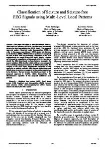
account a priori information pertinent to an application. This is achieved by using a set of positive real constants c1,.. .,c p , which have values directly proportional to the importance of the individual hypothesis. The constants can be set to attain a more powerful test. If the constants are all equal then this procedure reduces to the sequentially rejective Bonferroni test which the GSRBT is a generalisation of [5].The new p values are defined as Si= P i / c i . 3. Order the p values in ascendingorder, 5 S(2)5 .. . 5 and let c ( ~ and ) H(i)be the corresponding constants and hypotheses respectively. Also, let P ai = a/ C(j) . 4. The GSRBT, depicted in Figure 1, is performed as
follows: If S(l) > a1 then retain H ( l ) ,. . . , and stop; otherwise, reject H ( l ) and test the next hypothesis. This procedure is repeated until either all the hypotheses are rejected or a set of hypotheses is retained.
3.1. Generalised sequentially rejective Bonferroni test (GSRBT) The GSRBT was successfullyapplied to a signal processing problem in [9]. Eq (2) is defined for all time samples,
433
where U, is zero mean Gaussian with time dependent variance, ou( n ) ,The AR parameter a ( n ) gives a single pole rotating on the unit circle, i.e., a(n) = -0.99eJ2"fq(n) where
+--zGGxm Yes Reject H(
v
is the position of the pole on the unit circle for the first signal and
i i
-$&n+0.4 f i n - 0.3
Reject
05n5N/2-1 N/2 5 n 5 N - 1
(9)
is the pole position for the second signal. These signals were chosen because they have the same expected power at each time instant and the same frequency content over [0, N - 11. The S N R for the following experiments is calculated using
Accept
Figure 1. Generalised sequentially rejective Bonferroni test
5. Finally, a global decision is made based on the set 7-1 = { H ( i ) } of retained hypotheses. This decision will depend on the application. Now we will summarise the result given in [5] which proves the GSRBT maintains the the global significance level a. Consider a single hypothesis where Pr(Pi > ai) under the null hypothesis is equal to 1 - ai. It is this value ai which gives us confidence in our test. Similarly the objective of a multiple test procedure is to maintain the global level of significance over all the hypotheses. Let 1 be the set of indices of true null hypotheses, then the equivalent expression for forming a confidence interval for the GSRBT is [5]
This equation is shown to be true in [5] and therefore the global level of significance is maintained.
4. Simulations In this section we show results for the classification of two classes of first order time-varying autoregressive (TAR) signals. The classes are separable only in the time-frequency space. The TAR( 1) process is defined as:
434
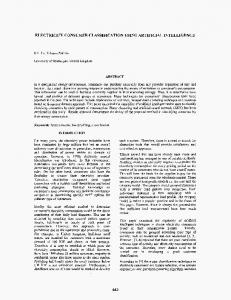
and &c are the variances of the real and imaginary parts of additive white Gaussian noise. To assess the performance of our method an Operating Characteristic (OC) curve was constructed for each class. We used 15 realisations from each class to estimate SI( n ,k) and SZ(n,k). The constants ci were set equal for these experiments. The OCs are shown in Figure 2. The matched filter and frequency spectrum method [7] naturally do not perform well for this class of signals. The template used for the matched filtering was an ensemble average calculated with 15 realisations of signals from each class. Figure 3 compares the classification performance of the multiple hypotheses method against a non-parametric time-frequency method that discriminates between classes using the distance between the log of the signal TFD and the log of the class TFDs [SI.
5. Discussion There is a number of optimisations which can be included for a particular application. The window length and the overlap used to estimate the TFDs in Eq's (2) and (3) can be optimised to reflect the degree of non-stationarity in the classes. The GSRBT can also be customised to an application. As mentioned in Section 3.1 the weights, c1,. . . ,c p , can be used to increase the power of the test and, in addition the accepted hypothesis can be combined in any arbitrary way to make a global decision. For example if two or more hypotheses are mutually exclusive, this information will influence the global decision. In Section 3.1 we assumed that the test statistics were normal, for narrowband signals this is not valid. The normal distribution is used to calculate the p values and therefore, is crucial to the performance of the test. In [7] it is shown that for narrowband signals the discriminant function in Eq (2) is
a summation of approximately chi-square random variables. This result can b e used to improve the performance of the algorithm [6]. The disadvantages with this method are twofold: firstly w e assume local stationarity to estimate the TFDs; and secondly, we assume that the signals are Gaussian. T h e method presented in [8], is non-parametric and so will be more appropriate if the Gaussian assurnption is not valid. Operating Characteristicsfor TimeAR(1) signids: SNR -1OdB , I
1
0.9 0.6
ProbaMlity of correct classification vs. SNR
Multiple Hypotheses
-
C
'50.73 0.6 E U
)
" . . l
-18
&
-16
-14
-12
-10 SNR (dB)
-8
-6
-4
class 2
Figure 3. Probability of correct classification Vs. SNR. Comparison of log TFD and multiple hypotheses methods.
".. g0.4 -9 -
Spectrum Method
5 0.3 P
0.1 o
0'
.
2 0.1
v 0.2
-
, , , 0.3 0.4 0.5 0.6 0.7 Probability of misclassilication
,
,
0.8
0.9
1
References
1
[l] S. Abeysekera and B. Boashash. Methods of signal classification using the images produced by the Wigner-Ville distributions. Pattern Recognition Letters, 12:717-729, Nov 1991. [2] B. Boashash. Time-frequency signal analyisis. In S . Haykin, editor, Advances in Spectrum Analysis, chapter 9. Prentice Hall, New Jersey, 199 1. [3] B. Boashash and P. O'Shea. A methodology for detection and classification of some underwater acoustics signals using time-frequency analysis techniques. IEEE Transactions on Acous,tics,Speech and Signal Processing, 38( 11):1829-1841, nov 1990. [4] Y. Hochberg and A. Tamhane. Multiple Comparison Procedures, page 363. John Wiley & Sons, United States of America, 1987. [SI S. Holm. A simple sequentially rejective multiple test procedure. Scand J Statist, 6:65-70, Nov 1979. [6] G. Roberts, A. Zoubir, and B. Boashash. Time-frequency discriminant analysis for non-stationary Gaussian signals. In Intem(ationa1Synposium on Signal Processing and its Applications, ISSPA'96, Gold Coast, Australia, 1996, Submitted. [7] R. Shumway. Discriminant analysis for time series. In P. Krishnaiah and L. Kanal, editors, Handbook of Statistics 2, chapter 1. North-Holland, New York, USA, 1982. [SI I. Vincent, C. Doncarli, and E. L. Carpentier. Non stationary signal classification using time-frequency distributions. In Timle-Frequencyand Time-ScaleAnalysis, pages 233-236, Philadelphia, USA, Oct 1994. [9] A. Zoubir and J. Bohme. Bootstrap multiple tests applied to sensor location. IEEE Transactions on Signal Processing, 43(6):1386-1396, June 1995.
Figure 2. OC for classification of the two signals: SNR = -1OdB. Comparison of matched filter, spectrum, log lFD, and multiple hypotheses methods.
6. Conclusion We have presented a new method for the classification of non-stationary Gaussian signals b:y combining timefrequency analysis with multiple hypothesis testing. A timefrequency distribution is used t o separate classes of signals that are inseparable in either the time or the frequency domain alone. T h e use of a multiple hypotheses test, the generalised sequentially rejective Bonferroni test (GSRBT), allowed the simultaneous treatment of the set o f test statistics that arise from the time-dependent discriminant function. T h e GSRBT can b e customised t o a particular application to increase the power of the test. T h e performance of this method was evaluated empirically by classifying two classes of zero mean non-stationary Gaussian signals. It performed favourably when compared t o the classical methods and another non-parametric timefrequency method. This gain in performance is dependent o n the Gaussian and local stationarity assumptions.
435