Fuzzy Connectivity Clustering with Radial Basis ... - Semantic Scholar

Fuzzy Connectivity Clustering with Radial Basis Kernel Functions Carl G. Looney† Abstract – We use a Gaussian radial basis kernel function to map pairs of feature vectors from a sample into a fuzzy connectivity matrix whose entries are fuzzy truths that the vector pairs belong to the same classes. To reduce the matrix size when the data set is large, we obtain a smaller set of representative vectors to form a smaller matrix. To this end we first group the feature vectors into many small pre-clusters based on summed feature-wise similarities, and then we use the pre-cluster centers as a reduced set of representatives. We next map the centers pair-wise to form the fuzzy connectivity matrix entries. When an unknown feature vector is input for classification, we find the nearest pre-cluster center and assign its class to the unknown vector. We demonstrate the method first on a simple set of linearly nonseparable synthetic data to show how it works and then apply it to the well known and difficult iris data and to the substantial and noisy Wisconsin breast cancer data. Keywords. Clustering, classification, fuzzy connectivity matrix, data reduction, kernel function _____________________________________________________________________________ † Computer Science & Engineering Department, Univ. of Nevada, Reno, Reno, NV 89557, U.S.A. Email: [email protected] Tel: 775-240-2920

Fax: 775-784-1877

1. INTRODUCTION Classifying a given set of feature vectors is a process of partitioning the set of feature vectors into classes, i.e., sub-populations, where the vectors are more alike within the classes and more different between classes. A partitioning of a data set of feature vectors into clusters of similar feature vectors is based on a similarity measure on pairs of feature vectors. Such partitioning can be done on unlabeled (unknown) data sets and thus is a form of self-organizing, i.e., unsupervised machine learning. Among many similarity measures that have been used are the Euclidean (most common), Minkowski, Mahalanobis, city-block, point symmetry and supremum distances, and more recently, the cosine similarity and correlation measures ( see Xu and Wunsch [1], 2005). Clustering is important and widely applicable for classification, pattern recognition, data mining, representation of large data sets by smaller representative sets (data abstraction), categorization of instances, document retrieval, image segmentation and dimensionality reduction. Classification via any algorithm requires features, or attributes, of the objects to distinguish their classes appropriately. A given clustering method may work well for certain data sets but not for others: there is no clustering algorithm that can correctly group all data sets. Different algorithms, and even the same algorithm with different parameter settings, may yield different clusterings of the same data, and humans may disagree on the classes. However, classification is critical for high level knowledge. For clustering overviews, see Xu and Wunsch [1], 2005, and Jain et al. [2], 1999. The goal here is to separate a data set into clusters, where the number K of classes (of one or more clusters each) may be unknown and so must be determined. Our method uses a kernel function to map each pair of feature vectors into an entry in a fuzzy connectivity that is the fuzzy truth that both vectors in the pair belong to the same class. The mapping takes the N-dimensional feature -2-

vector pairs of a set of Q such vectors into Q2 entries from 0 to 1 of a symmetric matrix. Entry values close to 0 designate strong separation and values close to 1 denote strong membership in the same class. We call our new similarity measure the kernel similarity. The pre-clustering is not necessary for generating the fuzzy connectivity matrix that does the actual clustering, but it reduces the matrix size considerably. Any method (e.g., k-means) may be used for pre-clustering, but when vectors contain noise this does not work well. Thus we use a more robust method that is more resistant to noise to perform the pre-clustering. Although the pre-clusters should be small in volume, there may be a large number of vectors in one or more of them. Before clustering a given set of N-dimensional feature vectors {x(q): q=1,...,Q}, where x(q) = (x1(q),...,xN(q)), it is usual to standardize the features by a linear mapping of each fixed feature n so its minimum value goes to 0 and its maximum value goes to 1 via xn(q) 6 (xn(q) - an) / ( bn - an) an = minq=1,Q {xn(q) },

(1)

bn = maxq=1,Q {xn(q) }

(2a,b)

This prevents features with larger ranges from dominating those of smaller ranges. Our preclustering and kernel mapping process automatically standardizes the fuzzy connectivity matrix (see Section 3) so we need not standardize the feature vectors. Section 2 presents the first stage that reduces the data by use of a new similarity that we designed to deal with noisy features. It finds many pre-clusters of small volume as a reduced representative set of vectors. Section 3 gives the main method of this paper, which is the mapping of pairs of pre-cluster centers into a fuzzy connectivity matrix. This can be done on the original feature vectors without any pre-clustering, but the matrix could be very large and unwieldy in that

-3-

case. In Section 4 we discuss the data sets and the results of computer runs on simple, but also on difficult, data sets that are substantial and noisy. Section 5 provides the conclusions. 2. THE PRE-CLUSTERING STAGE 2.1 Reducing the Data set for Efficiency The object of the pre-clustering first stage is to reduce a set of Q feature vectors to a smaller set of K vectors that represent the feature space. The pre-clusters must be small in volume (very similar) so that each is well represented by its center (a type of average or median vector). The number of pre-clusters is not so important, as we shall see, but we should not use too few. This first stage will be followed by the second stage where the fuzzy connectivity matrix of the pre-cluster centers is computed to connect those centers into clusters. The use of multiple pre-cluster centers as prototypes for a single class allows the class to have practically any shape and not be constrained by the shape of the unit ball of a distance function or other similarity measure. Given a set of Q feature vectors {x(q): q = 1,...,Q}, where each x(q) = (x1(q),...,xN(q)) has N features, the first stage reduces the data set by clustering the data set into pre-clusters of small volume and then computing a center of each pre-cluster to be put into the reduced set. We then map all unique pairs of these pre-cluster centers into the connectivity matrix in the second stage. 2.2 The First-stage Pre-clustering Algorithms Our pre-clustering method employs a similarity measure S(x, y) [3] that sums the number of approximate feature matches over the N features for each pair of N-dimensional vectors x = (x1,...,xN) and y = (y1,...,yN). Given N feature thresholds {tn: n = 1,...,N}, we compute (for each n # N) dn = 1 if | xn - yn | # tn,

dn = 0 if | xn - yn | > tn

(3a,b)

A user-given single proportion p (0 < p < 1) determines all feature thresholds {tn}n = 1,...,N as the -4-

proportion p of the ranges of the N features over the set of all feature vectors {x(q): q=1,...,Q}, where x(q) = (x1(q),...,xN(q)), via tn = (p)(range(n))

(4)

range(n) = maxq=1,Q {xn(q)} - minq=1,Q {xn(q)}

(5)

Our similarity measure S(x, y) is the sum S(x, y) = 3(n=1,N) dn SW(x, y) = 3(n=1,N) wndn

(6) [weighted version]

(7)

If the similarity satisfies S(x, y) > T1

(8)

for some similarity threshold T1 such that T1 # N (preferably closer to N if the error magnitudes are low), then we merge x and y into the same pre-cluster. Once T1 is set the user starts with a lower value for the proportion value of p and then iterates the pre-clustering [3] interactively by increasing p over the iterations until a usable set of pre-clusters is obtained for which the number K of pre-clusters is significantly larger than an estimate of the final number of classes. The value of p is a control to keep the pre-clusters compact. This summing of the feature-wise similarities is equivalent to voting by the features on the similarity between two vectors with T1 determining the required majority. Such feature voting is more robust to noise when T1 is much lower than N, and should work best for larger dimensionality where there can be enough features of relatively low noise in each instance to classify. Because a higher value of S indicates higher similarity, S(x, y) is a true similarity measure. We describe the algorithm in parts below.

-5-

Algorithm A - Set up the Pre-cluster Parameters Step 1: Input Q, N and Q feature vectors of N dimensions, {x(q): q = 1,...,Q} Read Q, put K = Q

//K is no. of initial singleton pre-clusters

For k = 1 to K do

//For each feature vector x(q) (q = k here)

Read x(k)

// read it into memory and then copy it to

Put c(k) = x(k)

// the center of a singleton initial pre-cluster

Step 2: Set up singleton pre-cluster assignments For k=1 to K do

//Assign each feature vector x(k) (K = Q)

clust[k] = k

// to its own pre-cluster no. k

count[k] = 1

// and set count of pre-cluster k to 1

Step 3: Compute the range of each feature (dimension) For n = 1 to N do Compute range[n] Input T1

//For each of N features (dimensions) // use Equation (5) //No. features to match for similarity, Eqn. (8)

Algorithm B - Merge Centers to Decrease Pre-cluster Centers Step 1: Compute all feature thresholds tn as proportion of ranges Input p

//Use small proportion p (say, 0.1) on first run, use it in

For n = 1 to N do

// Eqn. (4) ( increase p on later runs)

tn = p*range(n) Step 2: Assign each center to another center to which it is similar For k = 1 to K-1 do For kk = k+1 to K do

//Select each unique pair of pre-cluster // centers no.s k, kk and find their -6-

Compute S(c(kk), c(k))

// similarity by Eqns. (3a,b, and 6)

If S(c(k), c(kk )) $ T1 then //If similarity is high then change assignment For q = 1 to Q do // of each feature vector in pre-cluster kk to If clust[q] == kk do

// pre-cluster k, and then

clust[kk] = k

// and then increment and

count[k]++

// decrement the pre-cluster counts

count[kk]--

//Empty clusters are eliminated below

Step 3: Eliminate empty pre-clusters For k = 1 to K-1 do

//For each pre-cluster no. k, if it is

If count[k] 1 then

//Now divide center sum k by no. vectors // in pre-cluster k to get the average vector // components //This is the new center c(k)

c[n][k] = c[n][k]/count[k]

We prefer to compute the "-trimmed mean of each pre-cluster in Step 2 of Algorithm C rather than the mean so as to get rid of the worst outliers (see Bednar and Watt [4] 1984). This throws out the " largest and " smallest values of each feature n over any pre-cluster and averages the remaining ones. The median vector (with " = ƒK/2 - 1„) could also be used as a robust center. At this point we have the centers {c(k): k = 1,...,K} of pre-clusters of small volume that serve as a set of K representatives for the entire set of Q feature vectors {x(q): q = 1,...,Q}, where K < Q.

-8-

These centers are clustered in the second stage by mapping pairs of them into the fuzzy connectivity matrix. Our computer program is event driven from the keyboard where we enter a character to execute one of the algorithms A, B or C. We must execute A first to set up the parameters, and then we execute B and C in that order one or more times with different p values. Finally, we select D (see below) to compute the matrix. 3. THE FUZZY CONNECTIVITY STAGE 3.1 Kernel Mappings Any two classes of vectors in N-dimensional feature space are linearly separable if there is a hyperplane that separates the vectors in one class from those in the other class. Letting < , > denote the inner product, a hyperplane satisfies hw(x) = - b = w1x1 + . . . + wNxN - b = 0

(9)

The vectors x on the side where hw(x) > 0 belong to one class, the vectors x on the other side where hw(x) < 0 are in another class, and hw(x) = 0 for x in the hyperplane. The wn are the weights (coefficients) and b determines the position of the hyperplane along a line perpendicular to it. But in the case of the inside and outside, e.g., of an ellipsoid, no hyperplane can separate them, so they are called linearly non-separable. If an N-dimensional space is mapped nonlinearly into a higher dimensional space of dimension D > N, there may be hyperplanes that can separate the classes. Such separating hyperplanes would usually map inversely back into complex separating hypersurfaces in the original feature space. For example, in the original feature space there may be an ellipsoidal surface around the origin, inside of which is one class, while a second class is outside. But we don’t know the hypersurface mathematically (if we did then we would be done). -9-

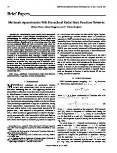
Our method derives from historical research in the classification and pattern recognition culture. Aizerman et al. [5], 1964, applied the kernel function of Mercer [6], 1909, to pattern recognition learning (classification). Such functions have been used in support vector machines (SVMs), principal component analysis (PCA) and other types of algorithms [7]. See [8, 9, 10] for SVMs and [11, 12, 13, 14] for kernel PCA. SVMs are quite accurate for many low-noise data sets, especially for a small number of classes and/or small dimension, but they can be numerically unstable in the case of an order of magnitude difference in feature values [7]. Kernel PCA can also be numerically unstable as shown by example in [7]. PCA was investigated by Pearson [15], 1901 and Hotelling [16], 1933, to find a set of fewer components that have maximal variance to reduce the dimension of data. In the example of Figure 1 there are 2 points inside the unit hypersphere x2 + y2 = 12 shown on the left side of the figure. That circle separates the plane into two regions with 2 points shown inside and 2 points outside. We map the circle boundary by g(x,y): (x,y) ÷ (u, v, w) to a line segment in 3 dimensions in (u,v,0) in the positive (first) octant. The hyperplane generated in (u, v, w) space by w (all values of w) for the line collinear to this segment separates the mapped vectors on the inside of the circle from those on the outside of the circle. The map is (x, y) ÷ g(x,y) = (u, v, w) = (|x|, |y|, 1 - x2 - y2)

(10)

If (x, y) is on the unit circle, then 1 = x2 + y2 so that w = 0 under the mapping. In general, it is difficult or impossible to find such facilitating mappings directly from the data. The two inside points in Figure 1 are mapped behind the hyperplane by (½, 0) 6 (½, 0, 3/4),

(0, ½) 6 (0, ½, 3/4)

and the two outside points are mapped to the front of the hyperplane according to -10-

(2,0) 6 (2, 0, -3),

(0, 2) 6 (0, 2, -3)

Figure 1. A simple separating map from 2 to 3 dimensions. 3.2 The Kernel Function Trick Because we can not use hyperplanes of the form = b in the original feature space to separate linearly non-separable classes, we want to: 1) map x 6 g(x) and w 6 g(w) nonlinearly into higher dimensions; and 2) separate classes with linearly separating hyperplanes via 5(w,x) = = b

(11)

The problem is that we don’t know what the function g(x) should be or how many dimensions are needed. However, we can define a nonlinear kernel function to be the radial basis function (RBF) G(-, -) as other researchers have done using similar functions. Thus we use 6 : úKxúK 6 ú

(12)

6(x(j),x(k)) = exp[-||x(j) - x(k)||2/(2F2)] = exp[-/(2F2)] = G()

(13)

where the width parameter is F > 0. This is used in place of 5(x(j),x(k)) =

(14) -11-

because the function g(x) is unknown. In other words, we take the nonlinear function of the inner product instead of the inner product of the (unknown) nonlinear function. This is known as the “kernel function trick.” It maps the hyperplanes nonlinearly into higher dimensions so as to separate classes. The function 6 changes the nonlinear problem into a linear problem, as happens in a radial basis function (RBF) neural network (NN), which is one type of support vector machine: the map from the input layer of N dimensions to the M-dimensional hidden layer nonlinearly maps the feature space to a higher M-dimensional space (M > N), and then the linear maps from the hidden layer to the output layer define hyperplanes that separate the M-dimensional space. Our method is a type of inversion of this. 3.3 The Second-stage Algorithm for the Fuzzy Connectivity Matrix This second stage starts with the K pre-cluster centers {c(k): k = 1,...,K} of dimension N that are to be mapped into K vectors of K dimensions each, N < K < Q. The radial basis kernel function maps each feature vector pair into a fuzzy connectivity truth. Let {c(1),...,c(K)} be the final set of K precluster centers that are representatives for the original data set {x(1),...,x(Q)}, where x(q) = (x1(q),...,xn(q)). We use G() to obtain yjk = 6(c(j),c(k)) = exp[-||c(j) - c(k)||2/(2F2)]

(15)

so as to form the matrix Y = [yjk] j=1,K; k=1,K

(fuzzy connectivity matrix)

Algorithm D - Generating the Fuzzy Connectivity Matrix Step 0: Input the data from the first stage Input K, Q, {c(k)}, {x(q)}

//These are from the first stage -12-

(16)

Compute F

//See Eqn. (17) below

Step 1: Compute the fuzzy connectivity matrix Adjust F

//User may increase/decrease or not change

For j = 1 to K do

//For each pair of pre-cluster centers

For k = j to K do Compute yjk

// compute fuzzy matrix entry j-k // using Equation (15)

Step 2: Set the fuzzy matrix threshold and use it on fuzzy connectivity matrix Input threshold T

//0.0 < T < 1.0, start at 0.5

For j = 1 to K do

//Use threshold to zero out

For k = j+1 to K do

// any small entries

If yjk < T then yjk = 0.0 Display yjk

//View results on screen

Step 3: User selects to re-do connectivity matrix or not User input selectKey

//Select to repeat or stop

If selectKey is repeat then

//If repeat, then go back and set

goto Step 1

// F (and T) again, get new matrix

Else write yjk to file

//Accept current connectivity matrix

Stop

// and quit program

In Equation (15) we find the width parameter F for the kernel function from the ranges (this is a subject for future research) by F2 = (1/N)3n=1,N [range(n)/(] 2

(17)

where ( (( = 2 is a good value to try) sets range. Larger ( yields a smaller F in Equation (15). -13-

By Equation (15), Y is symmetric. When j = k, then ykk = 1, but also if c(j) and c(k) are close, then yjk is near unity. On the other hand, if c(j) and c(k) are far apart, then yjk is near zero so it will be converted to zero by applying the threshold T. But near and far are determined to some extent by F and T, so the iterations through the loop allow experimentation on the data to obtain a fuzzy or crisp partitioning. More generally, the symmetric matrix Y is a correlation type matrix for the pre-cluster centers (correlation was used by Kohonen [17], 1982, as a similarity measure). Y is actually a fuzzy connectivity matrix because each yjk is a fuzzy truth value (between 0 and 1) for vectors j and k being in the same class: the radial basis function in Equation (15) is a fuzzy set membership function (FSMF) that c(j) belongs to the class of c(k). The fuzzy connectivity matrix is the final result. Some repetitions with increased or decreased values of F and T can be done for comparison before accepting the results that are rather insensitive to these values. Upon representing a data set of hundreds, or thousands, of feature vectors by, e.g., 10 to 30 pre-cluster centers, we reduce the fuzzy connectivity matrix dramatically. Our method is also immune to the order of the feature vectors (unlike k-means, for which a different order can yield different results). The combined pre-clusters can approximate a class of arbitrary shape. 3.4 Pattern Recognition with Fuzzy Connectivity Once we compute the fuzzy connectivity matrix Y then we can put any unknown feature vector x (from the same population as the original sample) into the system to check which pre-cluster it belongs to. Then we check the fuzzy connectivity matrix Y to determine which class that pre-cluster center belongs to and the fuzzy truths of such memberships. For crisp clustering, the pre-cluster centers can be grouped by the thresholded fuzzy connectivity matrix into core sets of prototypes (a

-14-

core set for each class). We need only store the strictly upper triangular part of the matrix Y and the set of pre-cluster centers. 3.4 Clustering Validity and the Number of Classes The number of classes K is very important parameter in clustering, yet it is often unknown. Clustering can be done for different K values where a clustering validity index (or validity measure) is applied to each result to select the final K value that provides the best validity value. Bezdek’s work [18] allows a feature vector to belong partially to each of multiple classes rather than only one, which originated the field of fuzzy clustering. The Xie-Beni (XB) fuzzy clustering validity (see [19], 1991) is often used to assess the clustering goodness. Also see Pal and Bezdek [20], 1995, for fuzzy clustering validity. The XB clustering validity for K clusters is given by XB = (1/K){3(k=1,K)Fk2 } / Dmin

(18)

Fk2 = 3{ (uqk )||x(q) - c(k)||2 : x(q) 0 Cluster k}

(19)

where Dmin is the minimum distance between cluster centers {c(k): k = 1,...,K} (the separation), and Fk2 is the mean-square error of Cluster k, and uqk is the fuzzy membership of x(q) in Cluster k (for crisp clustering, it is a 0 or 1). The numerator of Equation (18) is called the compactness of the clustering. The Kwon (Kw) validity index (see S. H. Kwon [21], 1998) appears to be as good, or slightly better, than the Xie-Beni validity. It changes the compactness and is given by Kw = (1/K){3(k=1,K)Fk2 + 3(k=1,K)||c(k) - :||2} / Dmin

(20)

where : is the mean of all Q feature vectors and c(k) is the center of the kth cluster. However, such validity indices involve a sum of mean-square errors (variances) of the clusters and thus are suited to (Euclidean) ball shaped clusters (hyperspheres), i.e., they are not valid for clusters of elongated, -15-

curved or other types of shapes. They are also biased toward a smaller K value. Other types of cluster validity indices exist (see [1, p. 665]). An important advantage of our method here is that we don’t need to compute any clustering validity to determine the number of classes because the fuzzy connectivity values are given in the matrix Y. We can find the row-wise maximum fuzzy truth that a vector connects to another vector. However, for comparison of experimental runs we can use a max-min fuzzy clustering validity for the fuzzy connectivity classes of our fuzzy connectivity matrix. First, we find the maximum nondiagonal entry (ORed value) fk within each row (unless all non-diagonal values are zero, in which case that single diagonal entry for a pre-cluster designates a class, so we use the diagonal entry; and second, we find the minimum (ANDed) value of all such maximum fuzzy truths fk between rows. We examine the fuzzy validities for two runs on the iris data set with different pre-clusters in the next section. 4. COMPUTER RUNS ON DATA SETS 4.1 Results on the 2-Dimensional test.dta Data set Figure 2 shows a synthetic linearly non-separable data set (test.dta), listed in Table 1, which is designed to fool clustering algorithms. We assume the number of classes K is unknown. Our algorithm first agglomerates all feature vectors into 10 small pre-clusters, finds their centers, and then computes a connectivity matrix for them. Figure 3 shows these results.

-16-

Fig 2. Original test data set.

Figure 3. Test results, 10 pre-clusters.

We also pre-clustered the test.dta data set into 8 pre-clusters with the results shown in Figure 4. After several experiments it appeared that the number of pre-clusters had no effect on the final classes for this data set, as long as it was large enough. The fuzzy threshold used on the matrix was T = 0.51. Figure 5 shows one result of k-means (given K = 2), but others varied with different sets of initial centers.

Fig. 4. Test results, 8 pre-clusters.

Fig. 5. Test results for k-means, K = 2.

-17-

Table 1. The test Data for Testing Vector PreNo . x y Class Cluster 1 2 3 4 5 6 7 8 9 10 11 12 13 14 15 16 17 18 19 20 21 22 23 24 25

1.000 1.500 2.000 3.000 3.000 3.500 4.500 5.500 5.000 6.500 7.000 7.000 4.000 3.500 4.000 4.000 4.500 5.000 5.500 8.500 9.000 9.000 9.000 9.000 9.500

7.000 7.500 8.000 9.000 10.00 9.500 8.500 8.500 9.000 7.500 8.000 7.000 6.000 5.500 4.500 3.000 3.500 3.500 2.500 6.500 6.000 5.500 3.500 4.000 4.000

1 1 1 1 1 1 1 1 1 1 1 1 2 2 2 2 2 2 2 1 1 1 1 1 1

1 1 1 2 2 2 3 3 3 4 4 4 5 5 6 7 7 7 8 9 9 9 10 10 10

Table 2 shows the 10x10 fuzzy connectivity matrix for the 10 pre-clusters shown in Table 3 and displayed in Figure 3. By using the pre-cluster centers, we reduced the matrix from 25x25 (625 entries) to 10x10 (100 entries) for 10 pre-clusters, for this case. The first row of Table 2 shows that pre-cluster centers 1 and 2 are connected; the second row shows that Pre-clusters 1, 2 and 3 are connected; from the third row we see that Pre-clusters 2, 3, and 4 are connected; and the fourth row shows that Pre-clusters 3, 4 and 9 are connected. The ninth and tenth rows show the connectivity of Pre-clusters 4, 9 and 10, and pre-clusters 9 and 10. Thus Preclusters 1, 2, 3, 4, 9, and 10 are all connected. On the other hand, rows 5, 6, 7, and 8 show that Preclusters 5, 6, 7, and 8 are connected (underlined). Thus K = 2 classes have been established from 10 pre-clusters per Figure 3 where K is not given. The class results were the same for 8 pre-clusters. -18-

Table 2. The Fuzzy Connectivity Matrix for test Data 1.00 0.52 0.00 0.00 0.00 0.00 0.00 0.00 0.00 0.00

0.52 1.00 0.67 0.00 0.00 0.00 0.00 0.00 0.00 0.00

0.00 0.67 1.00 0.63 0.00 0.00 0.00 0.00 0.00 0.00

0.00 0.00 0.63 1.00 0.00 0.00 0.00 0.00 0.54 0.00

0.00 0.00 0.00 0.00 1.00 0.85 0.54 0.00 0.00 0.00

0.00 0.00 0.00 0.00 0.85 1.00 0.85 0.54 0.00 0.00

0.00 0.00 0.00 0.00 0.54 0.85 1.00 0.85 0.00 0.00

0.00 0.00 0.00 0.00 0.00 0.54 0.85 1.00 0.00 0.00

0.00 0.00 0.00 0.54 0.00 0.00 0.00 0.00 1.00 0.63

0.00 0.00 0.00 0.00 0.00 0.00 0.00 0.00 0.63 1.00

Table 3. Pre-clusters for test.dta Data, 10 Pre-clusters Pre-Cluster Feature No. Class Count Vector No.s 1 2 3 4 5 6 7 8 9 10

1 1 1 1 2 2 2 2 1 1

3 3 3 3 2 1 3 1 3 3

1 2 3 4 5 6 7 8 9 10 11 13 14 15 16 17 19 20 21 23 24

12

18 22 25

We also computed the 25x25 fuzzy connectivity matrix for the 25 original feature vectors (as singleton pre-clusters) without merging any pre-clusters. While this full fuzzy connectivity matrix produced the same class results, the reduced matrices were easier to work with. The 25x25 matrix is displayed in Appendix B, which shows that the original feature vectors 13 - 19 (underlined bold italic) are in one class, and original feature vectors 1 - 12 and 20 - 24 make up the other class (bold). 4.2 Runs on the Iris Data The well-known iris data set is not separable into the 3 classes originally classified manually by Anderson [22], 1935. This data set can be obtained from the University of California, Irvine Machine Learning Repository [23]. This data set has the first 50 feature vectors with labels of 1, the second 50 with labels of 2 and the third 50 with labels of 3, but we rearranged the vectors to alternate -19-

labels 1, 2, 3, and repeat this throughout, and we numbered the vectors from 1 to 150. The iris data set is accepted to be a major difficult test for clustering algorithms. Its 150 feature vectors have 4 features that represent petal length, petal width, sepal length and sepal width of 3 species of iris flowers. Anderson labeled them into 3 classes of 50 samples each for the respective 3 species. The iris data can be learned fairly well by a radial basis function neural network or vector support machine because it is labeled, but neural networks and support vector machines learning systems learn mislabeled and noisy vectors as valid vectors and so will misclassify upon such incorrect learning. But self-organizing learning finds an inherent structure in the data, which may not agree with the given labels. It is now thought by many researchers that the iris data set contains two main classes (see [24], 2002; Lin and Lee [25], 1995; Billaudel et al. [26], 1999; Kim and Ramakrishna [27], 2005; and Wu and Yang [28], 2005). In [28], 5 of 8 validity indices showed 2 classes were the best, while the remaining 3 others showed 3, 5 and 8 classes, respectively, to be best. Thus the case of 3 classes was best in only 1 out of 8, yet this would be the result of training a NN or an SVM with the given labels. Figure 6 shows the fuzzy weighted average (FWA) [24] of each of the 4 iris features by classes obtained using Anderson’s labels. It can be seen that Feature 2 does not distinguish well between the classes and that small noise will contribute to overlapping of its values. Omitting it should improve the clustering. We can set T1 = 3 in the first stage so that only 3 of the 4 features must match well in Equations (6, 8).

Fig. 6. FWA of the four iris features. -20-

Table 4 lists the thresholded (T = 0.51) fuzzy connection matrix for the 8 obtained pre-clusters of the iris data for T1 = 3. Our feature vector numbers of the pre-clusters are shown in Table A-1 of Appendix A. The first pre-cluster has size 50 but low volume. It is a class by itself because no other pre-clusters are connected to it (the first row and first column are all 0s except for y11). All of the remaining pre-clusters, however, are connected and so belong to the same fuzzy connectivity class. We checked the first class and found that all of the 50 feature vectors labeled by Anderson as being in the first class are contained here in our first pre-cluster. The remaining 100 in the second class do not break into 2 classes of sizes 50 each (as labeled by Anderson) according to any clustering algorithms we know of in the literature. Table 4. Iris Data Fuzzy Connection Matrix, T1 = 3 1.00 0.00 0.00 0.00 0.00 0.00 0.00 0.00

0.00 1.00 0.78 0.72 0.96 0.67 0.84 0.58

0.00 0.78 1.00 0.00 0.85 0.90 0.00 0.00

0.00 0.72 0.00 1.00 0.78 0.00 0.87 0.77

0.00 0.96 0.85 0.78 1.00 0.70 0.79 0.52

0.00 0.67 0.90 0.00 0.70 1.00 0.00 0.00

0.00 0.84 0.00 0.87 0.79 0.00 1.00 0.90

0.00 0.58 0.00 0.77 0.52 0.00 0.90 1.00

The computer run on the iris data with T1 = 4 is shown in Table 5 (also see Table A-2 of Appendix A). Upon examination of the fuzzy connectivity matrix in Table 5 we see that the first class consists of pre-clusters 1,7, and 8, which together contain the 50 feature vectors labeled as the first class by Anderson. The remaining pre-clusters are all connected and thus make up the second class of 100 feature vectors that Anderson had labeled into two classes of size 50 each. It appears from Figure 6 that the second class is composed of two sets of respectively larger and small specimens of the same class (perhaps different soil nutrients made the difference).

-21-

Table 5. Iris Data Fuzzy Connection Matrix, T1 = 4

1.00 0.00 0.00 0.00 0.00 0.00 0.82 0.81

0.00 1.00 0.74 0.94 0.00 0.85 0.00 0.00

0.00 0.74 1.00 0.82 0.76 0.00 0.00 0.00

0.00 0.94 0.82 1.00 0.00 0.78 0.00 0.00

0.00 0.00 0.76 0.00 1.00 0.00 0.00 0.00

0.00 0.85 0.00 0.78 0.00 1.00 0.00 0.00

0.82 0.00 0.00 0.00 0.00 0.00 1.00 0.00

0.81 0.00 0.00 0.00 0.00 0.00 0.00 1.00

Upon comparing Tables 4 and 5 (T1 = 3 and 4, respectively), we obtain different values for our fuzzy validities. For T1 = 3 the minimum of the values max{0.78, 0.72, 0.96, 0.67, 0.84, 0.58}, max{0.78, 0.85, 0.90}, max{0.72, 0.78, 0.87, 0.77}, max{0.96, 0.85, 0.78, 0.70, 0.79, 0.52}, max{0.67, 0.90, 0.70}, max{0.84, 0.87, 0.79, 0.90}, max{0.58, 0.77, 0.52, 0.90} is f = 0.87. However, for the case of T1 = 4 the minimum of the row-wise maxima is 0.76 (from Row 5 of Table 5). This means that even though the final results of classes of 50 and 100 were the same, the T1 = 3 (where f = 0.87) case gave better pre-cluster centers to represent the fuzzy classes. 4.3 Runs on the Wisconsin Breast Cancer Data The wisc9-699 data set [23, 29, 30] has 699 records, of which the first field is the identification number. The next 9 fields contain the 9 features that have to do with properties of the hypothesis tissue: (1) clump thickness; (2) uniformity of cell size; (3) uniformity of cell shape; (4) marginal adhesion; (5) single epithelial cell size; (6) bare nuclei; (7) bland chromatin; (8) normal nucleoli; and (9) mitosis. The final field is the label, which is 2 for normal and 4 for malignant. Each of these 9 features takes values from 1 to 10. There are 458 records (feature vectors) with labels of 2 for normal and 241 with labels of 4 for malignant. Most clustering methods of which we are aware obtain far too many feature vectors in

-22-

the normal cluster and too few in the malignant class. The field values were judged and entered by humans and there is significant noise power, but we also believe there are a few incorrect labels. This is an extremely difficult data set to classify with self-organizing learning, but it is fairly easy to train a neural network or support vector machine to recognize an input vector as being in one or the other. However, we would have very little confidence in results from such an algorithm trained on such data. Table 6. Some Feature Vectors from the wisc9-699 Data Set. Our No.

ID No.

1 2 3 4 5 6 7 8 9 10 11 12 13 14 15 16 17 18 19 20 21 22 23 24 25 26

1041801 1043999 1044572 1047630 1049815 1050670 1050718 1054590 1054593 1056784 1057013 1059552 1065726 1066373 1071760 1072179 1080185 1081791 1084584 1096800 1091262 1099510 1100524 1002945 1102573 1103608

f1 f2 f3 f4 f5 f6 f7 f8 f9 5 3 3 3 2 3 4 4 1 1 1 1 1 2 3 3 1 1 8 7 5 10 7 9 5 5 4 7 4 6 4 6 1 4 3 1 4 1 1 1 2 1 3 1 1 10 7 7 6 4 10 4 1 2 6 1 1 1 2 1 3 1 1 7 3 2 10 5 10 5 4 4 10 5 5 3 6 7 7 10 1 3 1 1 1 2 1 2 1 1 8 4 5 1 2 12 7 3 1 1 1 1 1 2 1 3 1 1 5 2 3 4 2 7 3 6 1 3 2 1 1 1 1 2 1 1 2 1 1 1 2 1 3 1 1 10 7 7 3 8 5 7 4 3 10 10 10 8 6 1 8 9 1 6 2 1 1 1 1 7 1 1 5 4 4 9 2 10 5 6 1 6 6 6 9 6 12 7 8 1 2 5 3 3 6 7 7 5 1 10 4 3 1 3 3 6 5 2 6 10 10 2 8 10 7 3 3 5 4 4 5 7 10 3 2 1 5 6 5 6 10 1 3 1 1 10 10 10 4 8 1 8 10 1

Label 4 2 4 4 2 4 2 4 4 2 4 2 4 2 2 4 4 2 4 2 4 4 4 2 4 4

Table 6 shows some feature vectors that we selected from the data file. We note that one or more high feature values associate with malignant (label 4), while the others may be low, and so any two malignant feature vectors may be quite different on any similarity measure. Thus the usual similarities do not fare well here. Vector 20 has a label of 2 but its value of Feature 6 is 12, which is an obvious mistake (10 is the maximum value) and it is definitely mislabeled. -23-

If we compare the 1st and 13th vectors (label 4) with the 17th, 23rd, and 26th vectors (label 4) we see that they are very different. Further, 23rd and 26th vectors both have label 4 but they are far (in Euclidean distance) from, say, the 22nd and 25th vectors that also have label 4. The vectors with label 2 generally have small values. Table 7 shows the results of classifying the wisc9-699 data set with our algorithm using T1 = N = 9 (all features). The first pre-cluster of 471 feature vectors was somewhat compact and formed very early in the process (and remained constant as we increased p in very small increments). Preclusters 2 - 11 formed the second class in Table 7. On some runs, we tried to force the reduction in the number of pre-clusters used by increasing p too much, which put all, or almost all (on different runs) feature vectors into a single normal pre-cluster. This tells us that the normal pre-cluster has certain vectors that are quite similar to malignant ones and so connect to them when p increases a little too much.There were differences in the counts of our classes with the labeled classes, and also differences in the labels (e.g., if L vectors labeled 2 were classified by our method as being in the class with label 4 and L vectors labeled 4 were classified as label 2, it would not affect the counts). Table 7. Results on the wisc9-699 Data with T1 = 9. Pre-cluster No. Class No. Total No. of Vectors 1 1 471 2,3,4,5,7,9,11 2 222 6 3 2 8 4 1 10 5 1 12 6 2 We also made runs with T1 = 8 and T1 = 7. In the first of these cases, there were 494 vectors classified in the normal class, and in the second case there were 516. We found that the lower we put T1, the more quickly the normal class (the first pre-cluster) became larger. Upon looking at vectors

-24-

from the same labeled class, we found many of their features varied about as much as those with different class labels. Table 8 shows the results when we selected only 6 of 9 features (no.s 2, 3, 4, 6, 7, 8) to use (here T1 = 6 so that all 6 features were used). The first and fifth pre-clusters comprised the normal group, while the second, third, fourth, sixth and seventh pre-clusters made up the malignant group. The thresholded fuzzy connectivity matrix is shown in Table 9, where T = 0.34 (a larger F value increased the non-unity fuzzy entry values in a later run). Table 10 shows the differences between the labels and the classes found by our method. This means that we found 14 vectors in the malignant class (4) that were labeled normal, and 15 vectors in the normal class (2) that were labeled malignant. That gave an overall difference rate of 29/699 = 0.0415, or a 4% difference, which is about 2% false positive and 2% false negative. However, we are reasonably sure that some of the labels are incorrect and some data have significant errors. These results are for future comparison to those of other researchers on this difficult data set. Table 8. Results on the wisc9-699 Data with 6 Features Pre-cluster No. Class No. Total No. of Vectors 1 1 447 2 2 132 3 2 53 4 2 30 5 1 12 6 2 23 7 2 2 Class 1 total: 459 Class 2 total: 240

-25-

Table 9. The Thresholded Fuzzy Connectivity Matrix for 6 Features, wisc9-699 Data 1.000000

0.000000

0.000000

0.000000

0.681618

0.000000

0.000000

0.000000

1.000000

0.701849

0.442690

0.000000

0.372693

0.000000

0.000000

0.701849

1.000000

0.614846

0.000000

0.668216

0.000000

0.000000

0.442690

0.614846

1.000000

0.000000

0.603763

0.532708

0.681618

0.000000

0.000000

0.000000

1.000000

0.000000

0.000000

0.000000

0.372693

0.668216

0.603763

0.000000

1.000000

0.000000

0.000000

0.000000

0.000000

0.532708

0.000000

0.000000

1.000000

Table 10. Differences on the wisc9-699 Data, 6 Features and T1 = 6 Labeled Data Results of Our Method Labeled Class No. Vectors Class Found No. Vectors Differences* 2 (1) 458 1 459 15 4 (2) 241 2 240 14 * Differences between labels and classes found —————————————————————————————— 5. CONCLUSIONS This new method reduces a data set of feature vectors to be clustered by finding the centers of compact pre-clusters to use as representatives. This is the first stage. For this pre-clustering we use a special similarity function for noise suppression, but k-means (with Euclidean distance similarity) or other clustering could be used in this stage if the noise power is low and abundant pre-clusters of small volume are found. The second stage generates a fuzzy connectivity matrix with an entry for each pair of pre-cluster centers that is generated by a Gaussian kernel function used as a fuzzy set membership function. Pairs that belong to the same class have higher fuzzy truths. The number of classes K and the classes are found from the connectivity matrix. Upon starting with a small fuzzy threshold for the fuzzy connectivity matrix and increasing it if needed, we can obtain a partition of the pre-cluster centers into classes. The user can obtain, with few iterations, both the number K of the classes and the multiple prototypes (pre-cluster centers) of each class. -26-

The 150 iris feature vectors were respectively reduced to K = 10 and K = 8 pre-clusters with 10x10 and 8x8 and fuzzy connectivity matrices that both yielded K = 2 classes upon thresholding. The wisc9-699 data is very noisy but our method classified it with a 4% error from the labels, but it appears that the labels contain a few errors also. Strong advantages of this method are: (1) the number K of classes is determined correctly from the fuzzy connectivity matrix; (2) the ordering of the data have no effect on the results; (3) the shapes of the classes are constructed by the automatic adjoining of multiple centers and so are not constrained by a distance similarity measure; and (4) the order of merging and the order of the vectors do not affect the results. Our fuzzy clustering validity measure appears to be useful. We note that Ben-Hur et al. [31] used a support vector clustering algorithm with PCA that yielded K = 4 classes on the iris data set. Other spectral methods [13, 14] have done clustering on data with one cluster inside of another circular cluster, but only in 2-dimensional feature space. We entertain some doubts as to the capability of such methods on large data sets (see [2] for a discussion of what works and doesn’t work on large data sets).

-27-

REFERENCES [1] Rui Xu and Donald Wunsch, II, “Survey of clustering algorithms,” IEEE Trans. Neural Networks 16(3), 645 - 678, 2005. [2] A. K. Jain, N. N. Murty and P. J. Flynn, “Data clustering: a review,” ACM Computing Surveys 31(3), Sept., 263 - 323, 1999. [3] C. G. Looney, Classification: two stage clustering with ensemble fusion, Computer Science & Engineering Tech. Rpt., University of Nevada, Reno, Reno, NV 89557, May 2006. [4] J. B. Bedner and T. L. Watt, “Alpha-trimmed means and their relation to median filters,” IEEE Trans. Acoustics, Speech and Signal Processing 32(1), 145-153, 1984. [5] M. Aizerman, E. Braverman, and L. Rozonoer, “Theoretical foundations of the potential function method in pattern recognition learning,” Automation and Remote Control 25, 821-837, 1964. [6] James Mercer, “Functions of positive and negative type and their connection to the theory of integral equations,” Phil. Trans.Royal Soc. London A209, 415, 446, 1909. [7] Shawn Martin, The Numerical Stability of Kernel Methods. Technical Report, Sandia National Laboratory, New Mexico, November 3, 2005. [8] Vladimir Vapnik, Estimation of Dependencies Based on Empirical Data, Nauka. Moscow, 1979, English translation: Springer-Verlag, N.Y., 1982. [9] N. Cristianini and J. Shawe-Taylor, An Introduction to Support Vector Machines, Cambridge University Press, 2000. [10] Vladimir Vapnik, Statistical Learning Theory, Wiley-Interscience, New York, 1998. [11] B. Scholkopf, A. Smola and K.-R. Muller, “Nonlinear component analysis as a kernel eigenvalue problem,” Neural Computation 10, 1299 - 1319, 1998. -28-

[12] Y. Weiss, “Segmentation using eigenvectors: a unifying view,” Proc. IEEE Int. Conf. Computer Vision, 975 - 982, 1999. [13] A. Y. Ng, M. I. Jordan and Y. Weiss, “On spectral clustering: analysis and an algorithm,” in Advances in Neural Information Processing Systems 14, edited by T. Dietterich, S. Becker and Z.Ghahramani, MIT Press, Cambridge, 2002. [14] Y. Bengio, O. Delalleau, N. LeRoux, J.-F. Paiement, P. Vincent and M. Ouimet, “Learning eigenfunctions links spectral embedding and Kernel PCA, Neural Computat. 16, 2197 - 2219, 2004. [15] K. Pearson, “On lines of closest fit to systems of points in space,” Phil. Mag. 2, 1901, 559 - 572. [16] H. Hotelling, “Analysis of complex statistical variables into principal components,” J. Educational Psychology 24, 498 - 520, 1933. [17] T. Kohonen, “Self-organized formation of topologically correct feature maps,” Biol. Cybern. 43, 59 - 69, 1982. [18] J. C. Bezdek, Fuzzy Mathematics in Pattern Classification, Ph.D. Thesis, Center for Applied Mathematics, Cornell University, 1973. [19] X. L. Xie and G. Beni, “A validity measure for fuzzy clustering,” IEEE Transactions on Pattern Analysis and Machine Intelligence 13(8), 841 - 847, 1991. [20] N.R. Pal, J.C. Bezdek, "On cluster validity for the c-means model", IEEE trans. Fuzzy systems 3(3), 370-379, 1995. [21] S. H. Kwon, “Cluster validity index for fuzzy clustering,” Electronic Letters 34(22), 2176-2177, 1998. [22] E. Anderson, “The irises of the Gaspe peninsula,” Bull. American Iris Society 59, 2 - 5, 1935.

-29-

[23] UCI machine learning repository, University of California, Dept. Inf. Comput. Sci., Irvine, CA, www.ics.uci.edu/~mlearn/MLRepository.html . [24] Carl G. Looney, “Interactive clustering and merging with a new fuzzy expected value,” Pattern Recognition 35, 2413 - 2423, 2002. [25] C.-T. Lin and C.-S. George Lee, Neural Fuzzy Systems, Prentice-Hall, Upper Saddle River, NJ, 1995. [26] P. Billaudel, A. Devillez and G. V. Lecolier, “Performance evaluation of fuzzy classification methods designed for real time application,” Int’l J. Approx. Reasoning 20, 1 - 20, 1999. [27] M. Kim and R. S. Ramakrishna, “New indices for cluster validity assessment,” Pattern Recognition Letters 26, 2353 - 2363, 2005. [28] K.-L. Wu and M.-S. Yang, “A cluster index for fuzzy clustering,” Pattern Recognition Letters 26, 1275 - 1291, 2005. [29] O. L. Mangasarian and W. H. Wolberg, “Cancer diagnosis via linear programming,” SIAM News, 23(5), 1 - 18, Sept. 1990. [30] W. H. Wolberg and O. L. Mangasarian, “Multisurface method of pattern separation for medical diagnosis applies to breast cytology,” Proc. National Academy of Sciences, U.S.A. 87, 9193 - 9196, Dec. 1990. [31] A. Ben-Hur, D. Horn, H. Siegelmann and V. Vapnik, “Support vector clustering,” J. Machine Learning Research 2, 125 - 137, 2001.

-30-

Appendix A - Results of Clustering the Iris Data Table A-1. Iris Pre-cluster Numbers, T1 = 3 Pre-cluster 1 has 50 vectors numbered: 1 4 7 10 13 16 19 22 25 28 31 34 37 40 43 46 49 52 55 58 61 64 67 70 73 76 79 82 85 88 91 94 97 100 103 106 109 112 115 118 21 124 127 130 133 136 139 142 145 148 Pre-cluster 2 has 33 vectors numbered: 2 5 8 14 20 26 33 35 39 41 47 50 56 60 65 68 71 74 77 80 83 86 102 104 105 107 110 113 120 125 126 138 143 Pre-cluster 3 has 9 vectors numbered: 3 30 48 75 111 123 132 135 147 Pre-cluster 4 has 1 vectors numbered: 21 Pre-cluster 5 has 21 vectors numbered: 6 12 17 27 36 42 45 51 53 62 66 72 81 84 99 101 114 117 129 141 150 Pre-cluster 6 has 15 vectors numbered: 9 15 18 24 54 57 63 69 78 87 90 93 96 108 144 Pre-cluster 7 has 16 vectors numbered: 11 29 38 44 59 92 95 98 116 119 122 128 134 137 140 149 Pre-cluster 8 has 5 vectors numbered: 23 32 89 131 146 Class 1: pre-cluster 1 Class 2: pre-clusters 2 - 8 Table A-2. Iris Pre-cluster Numbers, T1 = 4 Pre-cluster 1 has 48 vectors numbered: 1 4 7 10 13 16 19 22 25 28 31 34 37 40 43 49 52 55 58 61 64 67 70 73 76 79 82 85 88 91 94 97 100 103 106 109 112 115 118 121 127 130 133 136 139 142 145 148 Pre-cluster 2 has 22 vectors numbered: 2 5 8 14 20 26 35 41 47 62 68 71 74 77 80 83 86 105 107 110 125 143 Pre-cluster 3 has 28 vectors numbered: 3 9 15 18 24 27 30 33 39 48 54 63 69 75 78 90 93 96 99 108 111 120 123 126 132 135 138 147 Pre-cluster 4 has 20 vectors numbered: 6 12 21 36 42 45 51 66 72 81 84 87 101 102 114 117 129 141 144 150 Pre-cluster 5 has 1 vectors numbered: 57 Pre-cluster 6 has 29 vectors numbered: 11 17 23 29 32 38 44 50 53 56 59 60 65 89 92 95 98 104 113 116 119 122 128 131 134 137 140 146 149 Pre-cluster 7 has 1 vectors numbered: 46 Pre-cluster 8 has 1 vectors numbered: 124 Class 1: pre-clusters 1, 7, 8 Class 2: pre-clusters 2, 3, 4, 5, 6

-31-

Appendix B. The 25x25 Fuzzzy Connection Matrix for the test.dta Data set 1. 2. 3. 4. 5. 6. 7. 8. 9. 10. 11. 12. 13. 14. 15. 16. 17. 18. 19. 20. 21. 22. 23. 24. 25.

1. 2. 3. 4. 5. 6. 7. 8. 9. 10. 11. 12. 13. 14. 15. 16. 17. 18. 19. 20. 21. 22. 23. 24. 25. 1.00 0.95 0.91 0.61 0.00 0.00 0.00 0.00 0.00 0.00 0.00 0.00 0.00 0.00 0.00 0.00 0.00 0.00 0.00 0.00 0.00 0.00 0.00 0.00 0.00 0.95 1.00 0.95 0.78 0.65 0.61 0.00 0.00 0.00 0.00 0.00 0.00 0.00 0.00 0.00 0.00 0.00 0.00 0.00 0.00 0.00 0.00 0.00 0.00 0.00 0.91 0.95 1.00 0.82 0.61 0.65 0.53 0.00 0.00 0.00 0.00 0.00 0.00 0.00 0.00 0.00 0.00 0.00 0.00 0.00 0.00 0.00 0.00 0.00 0.00 0.61 0.78 0.82 1.00 0.91 0.95 0.78 0.61 0.68 0.00 0.00 0.00 0.00 0.00 0.00 0.00 0.00 0.00 0.00 0.00 0.00 0.00 0.00 0.00 0.00 0.00 0.65 0.61 0.91 1.00 0.95 0.65 0.00 0.61 0.00 0.00 0.00 0.00 0.00 0.00 0.00 0.00 0.00 0.00 0.00 0.00 0.00 0.00 0.00 0.00 0.00 0.61 0.65 0.95 0.95 1.00 0.82 0.65 0.78 0.00 0.00 0.00 0.00 0.00 0.00 0.00 0.00 0.00 0.00 0.00 0.00 0.00 0.00 0.00 0.00 0.00 0.00 0.53 0.78 0.65 0.82 1.00 0.95 0.95 0.61 0.53 0.00 0.00 0.00 0.00 0.00 0.00 0.00 0.00 0.00 0.00 0.00 0.00 0.00 0.00 0.00 0.00 0.00 0.61 0.00 0.65 0.95 1.00 0.91 0.78 0.68 0.61 0.00 0.00 0.00 0.00 0.00 0.00 0.00 0.00 0.00 0.00 0.00 0.00 0.00 0.00 0.00 0.00 0.68 0.61 0.78 0.95 0.91 1.00 0.65 0.61 0.00 0.00 0.00 0.00 0.00 0.00 0.00 0.00 0.00 0.00 0.00 0.00 0.00 0.00 0.00 0.00 0.00 0.00 0.00 0.00 0.61 0.78 0.65 1.00 0.95 0.95 0.00 0.00 0.00 0.00 0.00 0.00 0.00 0.61 0.66 0.53 0.00 0.00 0.00 0.00 0.00 0.00 0.00 0.00 0.00 0.53 0.68 0.61 0.95 1.00 0.91 0.00 0.00 0.00 0.00 0.00 0.00 0.00 0.65 0.73 0.61 0.00 0.00 0.00 0.00 0.00 0.00 0.00 0.00 0.00 0.00 0.61 0.00 0.95 0.91 1.00 0.00 0.00 0.00 0.00 0.00 0.00 0.00 0.78 0.80 0.68 0.00 0.00 0.00 0.00 0.00 0.00 0.00 0.00 0.00 0.00 0.00 0.00 0.00 0.00 0.00 1.00 0.89 0.91 0.54 0.66 0.61 0.00 0.00 0.00 0.00 0.00 0.00 0.00 0.00 0.00 0.00 0.00 0.00 0.00 0.00 0.00 0.00 0.00 0.00 0.00 0.89 1.00 0.98 0.78 0.82 0.73 0.54 0.00 0.00 0.00 0.00 0.00 0.00 0.00 0.00 0.00 0.00 0.00 0.00 0.00 0.00 0.00 0.00 0.00 0.00 0.91 0.98 1.00 0.80 0.89 0.82 0.61 0.00 0.00 0.00 0.00 0.00 0.00 0.00 0.00 0.00 0.00 0.00 0.00 0.00 0.00 0.00 0.00 0.00 0.00 0.54 0.78 0.80 1.00 0.95 0.89 0.89 0.00 0.00 0.00 0.00 0.00 0.00 0.00 0.00 0.00 0.00 0.00 0.00 0.00 0.00 0.00 0.00 0.00 0.00 0.66 0.82 0.89 0.95 1.00 0.98 0.89 0.00 0.00 0.00 0.00 0.00 0.00 0.00 0.00 0.00 0.00 0.00 0.00 0.00 0.00 0.00 0.00 0.00 0.00 0.61 0.73 0.82 0.89 0.98 1.00 0.91 0.00 0.00 0.00 0.00 0.00 0.00 0.00 0.00 0.00 0.00 0.00 0.00 0.00 0.00 0.00 0.00 0.00 0.00 0.00 0.54 0.61 0.89 0.89 0.91 1.00 0.00 0.00 0.00 0.00 0.00 0.00 0.00 0.00 0.00 0.00 0.00 0.00 0.00 0.00 0.00 0.61 0.65 0.78 0.00 0.00 0.00 0.00 0.00 0.00 0.00 1.00 0.98 0.95 0.78 0.61 0.82 0.00 0.00 0.00 0.00 0.00 0.00 0.00 0.00 0.00 0.66 0.73 0.80 0.00 0.00 0.00 0.00 0.00 0.00 0.00 0.98 1.00 0.98 0.66 0.00 0.73 0.00 0.00 0.00 0.00 0.00 0.00 0.00 0.00 0.00 0.53 0.61 0.68 0.00 0.00 0.00 0.00 0.00 0.00 0.00 0.95 0.981.00 0.68 0.53 0.78 0.00 0.00 0.00 0.00 0.00 0.00 0.00 0.00 0.00 0.00 0.00 0.00 0.00 0.00 0.00 0.00 0.00 0.00 0.00 0.78 0.66 0.68 1.00 0.95 0.95 0.00 0.00 0.00 0.00 0.00 0.00 0.00 0.00 0.00 0.00 0.00 0.00 0.00 0.00 0.00 0.00 0.00 0.00 0.00 0.61 0.00 0.53 0.95 1.00 0.91 0.00 0.00 0.00 0.00 0.00 0.00 0.00 0.00 0.00 0.00 0.00 0.00 0.00 0.00 0.00 0.00 0.00 0.00 0.00 0.82 0.73 0.78 0.95 0.91 1.00

-32-