Clustering In A High-Dimensional Space Using Hypergraph Models ∗ Eui-Hong (Sam) Han
George Karypis
Vipin Kumar
Bamshad Mobasher Department of Computer Science and Engineering/Army HPC Research Center University of Minnesota 4-192 EECS Bldg., 200 Union St. SE Minneapolis, MN 55455, USA (612) 626 - 7503 fhan,karypis,kumar,
[email protected]
Abstract
Clustering of data in a large dimension space is of a great interest in many data mining applications. Most of the traditional algorithms such as K-means or AutoClass fail to produce meaningful clusters in such data sets even when they are used with well known dimensionality reduction techniques such as Principal Component Analysis and Latent Semantic Indexing. In this paper, we propose a method for clustering of data in a high dimensional space based on a hypergraph model. The hypergraph model maps the relationship present in the original data in high dimensional space into a hypergraph. A hyperedge represents a relationship (affinity) among subsets of data and the weight of the hyperedge reflects the strength of this affinity. A hypergraph partitioning algorithm is used to find a partitioning of the vertices such that the corresponding data items in each partition are highly related and the weight of the hyperedges cut by the partitioning is minimized. We present results of experiments on three different data sets: S&P500 stock data for the period of 1994-1996, protein coding data, and Web document data. Wherever applicable, we compared our results with those of AutoClass and K-means clustering algorithm on original data as well as on the reduced dimensionality data obtained via Principal Component Analysis or Latent Semantic Indexing scheme. These experiments demonstrate that our approach is applicable and effective in a wide range of domains. More specifically, our approach performed much better than traditional schemes for high dimensional data sets in terms of quality of clusters and runtime. Our approach was also able to filter out noise data from the clusters very effectively without compromising the quality of the clusters. Keywords: Clustering, data mining, association rules, hypergraph partitioning, dimensionality reduction, Principal Component Analysis, Latent Semantic Indexing.
∗ This work was supported by NSF ASC-9634719, by Army Research Office contract DA/DAAH04-95-1-0538, by Army High Performance Computing Research Center cooperative agreement number DAAH04-95-2-0003/contract number DAAH04-95-C-0008, the content of which does not necessarily reflect the position or the policy of the government, and no official endorsement should be inferred. Additional support was provided by the IBM Partnership Award, and by the IBM SUR equipment grant. Access to computing facilities was provided by AHPCRC, Minnesota Supercomputer Institute. See http://www.cs.umn.edu/∼han for other related papers.
1 Introduction Clustering in data mining [SAD+ 93, CHY96] is a discovery process that groups a set of data such that the intracluster similarity is maximized and the intercluster similarity is minimized [CHY96]. These discovered clusters are used to explain the characteristics of the data distribution. For example, in many business applications, clustering can be used to characterize different customer groups and allow businesses to offer customized solutions, or to predict customer buying patterns based on the profiles of the cluster to which they belong. Given a set of n data items with m variables, traditional clustering techniques [NH94, CS96, SD90, Fis95, DJ80, Lee81] group the data based on some measure of similarity or distance between data points. Most of these clustering algorithms are able to effectively cluster data when the dimensionality of the space (i.e., the number of variables) is relatively small. However, these schemes fail to produce meaningful clusters, if the number of variables is large. Clustering of data in a large dimension space is of a great interest in many data mining applications. For example, in market basket analysis, a typical store sells thousands of different items to thousands of different customers. If we can cluster the items sold together, we can then use this knowledge to perform effective shelf-space organization as well as target sales promotions. Clustering of items from the sales transactions requires handling thousands of variables corresponding to customer transactions. Finding clusters of customers based on the sales transactions also presents a similar problem. In this case, the items sold in the store correspond to the variables in the clustering problem. One way of handling this problem is to reduce the dimensionality of the data while preserving the relationships among the data. Then the traditional clustering algorithms can be applied to this transformed data space. Principal Component Analysis (PCA) [Jac91], Multidimensional Scaling (MDS) [JD88] and Kohonen Self-Organizing Feature Maps (SOFM) [Koh88] are some of the commonly used techniques for dimensionality reduction. In addition, Latent Semantic Indexing (LSI) [BDO95] is a method frequently used in the information retrieval domain that employs a dimensionality reduction technique similar to PCA. An inherent problem with dimensionality reduction is that in the presence of noise in the data, it may result in the degradation of the clustering results. This is partly due to the fact that by projecting onto a smaller number of dimensions, the noise data may appear closer to the clean data in the lower dimensional space. In many domains, it is not always possible or practical to remove the noise as a preprocessing step. Furthermore, as we discuss in Section 2, most of these dimensionality reduction techniques suffer from shortcomings that could make them impractical for use in many real world application domains.
1
In this paper, we propose a method for clustering of data in a high dimensional space based on a hypergraph model. In a hypergraph model, each data item is represented as a vertex and related data items are connected with weighted hyperedges. A hyperedge represents a relationship (affinity) among subsets of data and the weight of the hyperedge reflects the strength of this affinity. Now a hypergraph partitioning algorithm is used to find a partitioning of the vertices such that the corresponding data items in each partition are highly related and the weight of the hyperedges cut by the partitioning is minimized. The relationship among the data points can be based on association rules [AS94] or correlations among a set of items [BMS97], or a distance metric defined for pairs of items. In the current version of our clustering algorithm, we use frequent item sets found using Apriori algorithm [AS94] to capture the relationship, and hypergraph partitioning algorithm HMETIS [KAKS97] to find partitions of highly related items in a hypergraph. Frequent item sets are derived by Apriori, as part of the association rules discovery, that meet a specified minimum support criteria. Association rule algorithms were originally designed for transaction data sets, where each transaction contain a subset of the possible item set I . If all the variables in the data set to be clustered are binary, then this data can be naturally represented as a set of transactions as follows. The set of data items to be clustered becomes the item set I , and each binary variable becomes a transaction that contains only those items for which the value of the variable is 1. Non-binary discrete variables can be handled by creating a binary variable for each possible value of the variable. Continuous variables can be handled once they have been discretized using the techniques similar to those presented in [SA96]. Association rules are particularly good in representing affinity among a set of items where each item is present only a small fraction of the transactions and presence of an item in a transaction is more significant than the absence of the item. This is true for all the data sets used in our experiments. To test the applicability and robustness of our scheme, we evaluated it on a wide variety of data sets [HKKM97a, HKKM97b]. We present results on three different data sets: S&P500 stock data for the period of 1994-1996, protein coding data, and Web document data. Wherever applicable, we compared our results with those of AutoClass [CS96] and K-Means clustering algorithm on original data as well as on the reduced dimensionality data obtained via PCA or LSI. These experiments demonstrate that our approach is applicable and effective in a wide range of domains. More specifically, our approach performed much better than traditional schemes for high dimensional data sets in terms of quality of clusters and runtime. Our approach was also able to filter out noise data from the clusters very effectively
2
without compromising the quality of the clusters. The rest of this paper is organized as follows. Section 2 contains review of related work. Section 3 presents our clustering method based on hypergraph models. Section 4 presents the experimental results. Section 5 contains conclusion and directions for future work.
2 Related Work Clustering methods have been studied in several areas including statistics [DJ80, Lee81, CS96], machine learning [SD90, Fis95], and data mining [NH94, CS96]. Most of the these approaches are based on either probability, distance or similarity measure. These schemes are effective when the dimensionality of the data is relatively small. These scheme tend to break down when the dimensionality of the data is very large for several reasons. First, it is not trivial to define a distance measure in a large dimensional space. Secondly, distance-based schemes generally require the calculation of the mean of document clusters or neighbors. If the dimensionality is high, then the calculated mean values do not differ significantly from one cluster to the next. Hence the clustering based on these mean values does not always produce good clusters. Similarly, probabilistic methods such as Bayesian approach used in AutoClass [CS96], do not perform well when the size of the feature space is much larger than the size of the sample set, which is common in many large dimensional data sets. Furthermore, the underlying expectation-maximization (EM) algorithm [TSM85] in AutoClass has the computational complexity of O(kd 2 n I ) where k is the number of clusters, d is the number of attributes, n is the number of items to be clustered, and I is the average number of iterations of the EM algorithm. Hence, for large dimensional data sets, AutoClass’ run time can be unacceptably high. A well-known and widely used technique for dimensionality reduction is Principal Component Analysis (PCA) [Jac91]. Consider a data set with n data items and m variables. PCA computes a covariance matrix of size m × m, and then calculate the k leading eigenvectors of this covariance matrix. These k leading eigenvectors of this matrix are principal features of the data. The original data is mapped along these new principal directions. This projected data has lower dimensions and can now be clustered using traditional clustering algorithms such as K-means [JD88], Hierarchical clustering [JD88], or AutoClass. PCA provides several guidelines on how to determine the right number of dimension k for given data based on the proportion of variance explained or the characteristic roots of the covariance matrix. However, as noted in [Jac91], different methods provide widely different guideline for k on the same data, and thus it can be dif-
3
ficult to find the right number of dimension. The choice of small k can lose important features of the data. On the other hand, the choice of large k can capture most of the important features, but the dimensionality might be too large for the traditional clustering algorithms to work effectively. Another disadvantage of PCA is that its memory requirement is O(m 2 ) and computational requirement is higher than O(m 2 ) depending on the number of eigenvalues. These requirements can be unacceptably high for large m. Latent Semantic Indexing (LSI) [BDO95] is a dimensionality reduction technique extensively used in information retrieval domain and is similar in nature to PCA. Instead of finding the singular value decomposition of the covariance matrix, it finds the singular value decomposition of the original n × m data. Since LSI does not require calculation of the covariance matrix, it has smaller memory and CPU requirements when n is less than m [Jac91]. The Kohonen Self-Organizing Feature Map (SOFM) [Koh88] is a scheme based on neural networks that projects high dimensional input data into a feature map of a smaller dimension such that the proximity relationships among input data are preserved. Each neuron in the competitive layer of this approach competes with one another for the best stimulus response in terms of similarity to the input data, and the winning neuron and its neighbor neurons update their weight vectors in the direction such that these weight vectors become more similar to the input data. After the network is trained, each data point is projected on to these neurons according to the best match with weight vectors of the neurons. SOFM does not provide a measure of how good the transformation is. Furthermore, on data sets with very large dimensions, convergence in the network training could be very slow. Multidimensional Scaling (MDS) [JD88] transforms original data into a smaller dimensional space while trying to preserve the rank ordering of the distances among data points. MDS does not provide any good guidelines on how to find the right number of dimension to capture all the variations in the original data. Furthermore many of these techniques have high computational complexity of O(n 2 ) where n is the number of items being clustered. The use of hypergraphs in data mining has been studied recently. For example in [GKMT97] it is shown that the problem of finding maximal elements in a lattice of patterns is closely related to the hypergraph transversal problem [EG95]. The clustering or grouping of association rules have been proposed in [TKR+ 95], [LSW97] and [KA96]. In [TKR+ 95] and [LSW97], the focus is on finding clusters of association rules that have the same right hand side rather than on finding item clusters. In [KA96], a scheme is proposed to cluster database attributes based on binary associations. In this approach, the association graph is constructed by taking attributes in a database as vertex set and con-
4
sidering binary associations among the items as edges in the graph. The minimum spanning tree (MST) is constructed and the edges in the minimum spanning tree are proposed as the most interesting associations. Successive removal of edges from the minimum spanning tree is used to produce clusters of attributes [KA96, JD88]. Since the MST algorithm only focuses on finding a set of edges to connect all the vertices while minimizing the sum of these weights, the resulting minimum spanning tree does not have information on the density of edges connecting related vertices. This information is essential in finding good clusters. Hence, MST-based scheme may not produce good quality clusters. Since graph partitioning algorithms implicitly take into account the density of interconnectivity of vertices, they are better candidates for finding clusters.
3 Hypergraph-Based Clustering Our algorithm for clustering related items consists of the following two steps. During the first step, a weighted hypergraph H is constructed to represent the relations among different items, and during the second step, a hypergraph partitioning algorithm is used to find k partitions such that the items in each partition are highly related. In our current implementation, we use frequent item sets found by the association rule algorithm [AS94] as hyperedges. We first present a brief overview of association rules that are used to model the information in a transaction database as a hypergraph, and then describe the hypergraph modeling and the clustering algorithm.
3.1 Association Rules Association rules capture the relationship of items that are present in a transaction [AMS+ 96]. Let T be the set of transactions where each transaction is a subset of the item-set I . Let C be a subset of I , then we define the support count of C with respect to T to be: σ (C) = |{t|t ∈ T, C ⊆ t}|.
Thus σ (C) is the number of transactions that contain C. For example, consider a set of transactions from supermarket as shown in Table 1. The items set I for these transactions is fBread, Beer, Coke, Diaper, Milkg. The support count of fDiaper, Milkg is σ (Di aper, Milk) = 3, whereas σ (Di aper, Milk, Beer ) = 2. s,α
An association rule is an expression of the form X H⇒ Y , where X ⊆ I and Y ⊆ I . The support s of the rule s,α
X H⇒ Y is defined as σ (X ∪ Y )/|T |, and the confidence α is defined as σ (X ∪ Y )/σ (X). For example, consider a rule 5
TID 1 2 3 4 5
Items Bread, Coke, Milk Beer, Bread Beer, Coke, Diaper, Milk Beer, Bread, Diaper, Milk Coke, Diaper, Milk
Table 1: Transactions from supermarket.
fDiaper, Milkg H⇒ fBeerg, i.e. presence of diaper and milk in a transaction tends to indicate the presence of beer in the transaction. The support of this rule is
σ (Diaper,Milk,Beer) 5
= 0.40. The confidence of this rule is
σ (Diaper,Milk,Beer) σ (Diaper,Milk)
=
0.66. Rules with high confidence (i.e., close to 1.0) are important, because they denote a strong correlation of the items in the rule. Rules with high support are important, since they are supported by a non-trivial fraction of transactions in the database. s,α
The task of discovering an association rule is to find all rules X H⇒ Y , such that s is greater than a given minimum support threshold and α is greater than a given minimum confidence threshold. The association rule discovery is composed of two steps. The first step is to discover all the frequent item-sets (candidate sets that have support greater than the minimum support threshold specified). The second step is to generate association rules from these frequent item-sets. A number of algorithms have been developed for discovering frequent item-sets [AIS93, AS94, HS95]. Apriori algorithm presented in [AS94] is one of the most efficient algorithms available. This algorithm has been experimentally shown to be linearly scalable with respect to the size of the database [AS94], and can also be implemented on parallel computers [HKK97b] to use their large memory and processing power effectively.
3.2 Hypergraph Modeling A hypergraph [Ber76] H = (V, E) consists of a set of vertices (V ) and a set of hyperedges (E). A hypergraph is an extension of a graph in the sense that each hyperedge can connect more than two vertices. In our model, the set of vertices V corresponds to the set of data items being clustered, and each hyperedge e ∈ E corresponds to a set of related items. A key problem in modeling of data items as hypergraph is the determination of related items that can be grouped as hyperedges and determining weights of each such hyperedge. The frequent item sets computed by an association rule algorithm such as Apriori are excellent candidates to find
6
support{A} = 0.25 support{B} = 0.25 support{C} = 0.25
B
A
C
support{A,B} = 0.1 support{B,C} = 0.1 support{A,C} = 0.1
P(A|B) = P(B|A) = 0.4 P(B|C) = P(C|B) = 0.4 P(A|C) = P(C|A) = 0.4
support{A,B,C} = 0.1
P(A|BC) = P(B|AC) = P(C|AB) = 1.0
Figure 1: Illustration of the power of confidence in capturing relationships among items. such related items. Note that these algorithms only find frequent item sets that have support greater than a specified threshold. The value of this threshold may have to be determined in a domain specific manner. The frequent item sets capture relationship of items of size greater than or equal to 2. Note that distance based relationships can only capture relationship among pairs of data points whereas the frequent items sets can capture relationship among larger sets of data points. This added modeling power is nicely captured in our hypergraph model. Assignment of weights to the resulting hyperedges is more tricky. One obvious possibility is to use the support of each frequent item set as the weight of the corresponding hyperedge. Another possibility is to make the weight as a function of the confidence of the underlying association rules. For size two hyperedges, both support and confidence provide similar information. In fact, if two items A and B are present in equal number of transactions (i.e., if the support of item set fAg and item set fBg are the same), then there is a direct correspondence between the support and the confidence of the rules between these two items (i.e., greater the support for fA, Bg, more confidence for rules “ fAg H⇒ fBg” and “fAg H⇒ fBg”). However, support carries much less meaning for hyperedges of size greater than two, as in general, the support of a large hyperedge will be much smaller than the support of smaller hyperedges. Furthermore, for these larger item sets, confidence of the underlying association rules can capture correlation among data items that is not captured by support. For example, consider three items A, B and C and their relationship as represented in Figure 1. The support of each of the pairs fA, Bg, fB, Cg and fA, Cg is 0.1, and the support of fA, B, Cg is also 0.1. However, the three-way relationship among A, B and C is much stronger than those among pairs, as P(C|AB), P(B|AC) and P(A|BC) are all 1.0. These conditional probabilities are captured in the confidence of corresponding association rules. This example also illustrates that relationships among item sets of size greater than 2 cannot always be captured by the pairwise relationships of its subsets irrespective of whether the relationship is modeled by the support or the confidence of the individual rules. Hence, a hypergraph is a more expressive model than a graph for this problem.
7
Another, more natural, possibility is to define weight as a function of the support and confidence of the rules that are made of a group of items in a frequent item set. Other options include correlation, distance or similarity measure. In our current implementation of the model, each frequent item-set is represented by a hyperedge e ∈ E whose weight is equal to the average confidence of the association rules, called essential rules, that have all the items of the edge and has a singleton right hand side. We call them are essential rules, as they capture information unique to the given frequent item set. Any rule that has only a subset of all the items in the rule is already included in the rules of subset of this frequent item set. Furthermore, all the rules that have more than 1 item on the right hand size are also covered by the subset of the frequent item set. For example, if fA,B,Cg is a frequent item-set, then the hypergraph contains a hyperedge that connects A, B, and C. Consider a rule fAgH⇒fB,Cg. Interpreted as an implication rule, this information is captured by fAgH⇒fBg and fAgH⇒fCg. Consider the following essential rules (with confidences 0.4
0.6
0.8
noted on the arrows) for the item set fA,B,Cg: fA,BgH⇒fCg, fA,CgH⇒fBg, and fB,CgH⇒fAg. Then we assign weight of 0.6 ( 0.4+0.6+0.8 = 0.6) to the hyperedge connecting A,B, and C. We will refer to this hypergraph as the 3 association-rule hypergraph.
3.3 Finding Clusters of Items Note that the frequent items sets already represent relationship among the items of a transaction. But these relationships are “fine grain”. For example, consider the following three frequent item sets found from a database of stock transactions:
fTexas Inst↑, Intel↑, Micron Tech↑g fNational Semiconduct↑, Intel↑g fNational Semiconduct↑,Micron Tech↑g These item sets indicate that on many different days, stocks of Texas Instrument, Intel and Micron Technology moved up together, and on many days, stocks of Intel and National Semiconductor moved up together, etc. From these, it appears that Texas Instrument, Intel, Micron Technology and National Semiconductor are somehow related. But a frequent item set of these four stocks may have small support and may not be captured by the association rule computation algorithm.
8
However the hypergraph representation can be used to cluster together relatively large groups of related items by partitioning it into highly connected partitions. One way of achieving this is to use a hypergraph partitioning algorithm that partitions the hypergraph into two parts such that the weight of the hyperedges that are cut by the partitioning is minimized. Note that by minimizing the hyperedge-cut we essentially minimize the relations that are violated by splitting the items into two groups. Now each of these two parts can be further bisected recursively, until each partition is highly connected. HMETIS is a multi-level hypergraph partitioning algorithm that has been shown to produce high quality bi-sections on a wide range of problems arising in scientific and VLSI applications. HMETIS minimizes the weighted hyperedge cut, and thus tends to create partitions in which the connectivity among the vertices in each partition is high, resulting in good clusters. Once, the overall hypergraph has been partitioned into k parts, we eliminate bad clusters using the following cluster fitness criterion. Let e be a set of vertices representing a hyperedge and C be a set of vertices representing a partition. The fitness function that measures the goodness of partition C is defined as follow: P e⊆C W eight (e) f i tness(C) = P |e∩C|>0 W eight (e)
The fitness function measures the ratio of weights of edges that are within the partition and weights of edges involving any vertex of this partition. The high fitness value suggests that the partition has more weights for the edges connecting vertices within the partition. The partitions with fitness measure greater than a given threshold value are considered to be good clusters and retained as clusters found by our approach. In our experiments, we set this fitness threshold to 0.1. Note that this fitness criterion can easily be incorporated into a partitioning algorithm such that each partition is further bisected only if the fitness of the partition is below the given threshold value. Then all the partitions found can be considered good partitions. Once good partitions are found, each good partition is examined to filter out vertices that are not highly connected to the rest of the vertices of the partition. The connectivity function of vertex v in C is defined as follow:
connecti vi t y(v, C) =
9
|{e|e ⊆ C, v ∈ e}| |{e|e ⊆ C}|
The connectivity measures the percentage of edges that each vertex is associated with. High connectivity value suggests that the vertex has many edges connecting good proportion of the vertices in the partition. The vertices with connectivity measure greater than a give threshold value are considered to belong to the partition, and the remaining vertices are dropped from the partition. In our experiments, we set this connectivity threshold to 0.1.
3.4 Computational Complexity The problem of finding association rules that meet a minimum support criterion has been shown to be linearly scalable with respect to the number of transactions [AMS+ 96]. Highly efficient algorithms such as Apriori are able to quickly find association rules in very large databases provided the support is high enough. For example, our experiments with Apriori have shown that for a data set of 1 million transactions each containing a subset of 1000 items can be found in a few minutes. Note that the computational requirement increases dramatically if the minimum support decreases. In our scheme, we do not need to find all the association rules with very low support. We only need to find right amount of information from the association rules so that we can cluster the items. If the minimum support is too low, then we will capture too many minor relationships among data points, most of which could be noise. Furthermore, our hypergraph partitioning algorithm [KAKS97] can find good partitions only if the hypergraph is reasonably sparse. Thus by keeping the support threshold high enough, we can limit the computational complexity of the Apriori algorithm. Hypergraph partitioning is a well studied problem in the context of VLSI circuit partitioning and highly efficient algorithms such as HMETIS have been recently developed [KAKS97]. This algorithm can find very good bisection of circuits containing over 100,000 nodes in a few minutes on a workstation. In particular, the complexity of HMETIS for a k-way partitioning is O((V + E) log k) where V is the number of vertices and E is the number of edges. The number of vertices in an association-rule hypergraph is the same as the number of data items to be clustered. The number of hyperedges is the same as the number of frequent item-sets with support greater than the specified minimum support. Note that the number of frequent item sets (i.e., hyperedges) does not increase as the number of transactions (i.e., variables) increases. Hence, our clustering method is linearly scalable with respect to the number of variables (i.e., the dimension of the data).
10
4 Experimental Results We tested the ability of our item-clustering algorithm to find groups of related items, on data-sets from many application areas. The results of these experiments are described in the following subsections. We have compared our results with that of AutoClass and K-means algorithm on the raw data and also compared the result of K-means on the reduced dimensionality data produced using PCA and LSI. We chose AutoClass for comparison because AutoClass can find the right number of clusters automatically, and is known for producing good quality clusters. For distance-based clustering, we chose K-Means algorithm for comparison, since it is one of the well known distance-based clustering algorithms. In all experiments with PCA and LSI schemes, data was normalized appropriately. PCA, LSI, and K-means were performed for many values of the parameters used by these algorithms (such as number of dimensions and the number of clusters). We report only the best results found. In all of our experiments, we used a locally implemented version of Apriori algorithm [AS94] to find the association rules and construct the association-rule hypergraph.
4.1 S&P 500 Stock Data Our first data-set consists of the daily price movement of the stocks that belong to the S&P500 index. It is well known in the financial community, that stocks belonging to the same industry group tend to trade similarly. For example, a group of stocks from a particular industry tend to move up or down together depending on the market’s belief about the health of this industry group. For this reason, we used this data set to verify the ability of our clustering algorithm to correctly cluster the various stocks according to their industry group. Our data set consists of a binary table of size 1000×716. Each row of this table corresponds to up or down movement indicator for one of the 500 stocks in S&P500 stocks, and each column corresponds to a trading day from Jan. 1994 to Oct. 1996. An entry of 1 in location (i, j ) where i corresponds to up indicator of a stock means that the closing price of this stock on j -th day is significantly higher (2% or 1/2 point or more) than the day before. Similarly, an entry of 1 in location (i, j ) where i corresponds to down indicator of a stock means that the closing price of this stock on j -th day is significantly lower (2% or 1/2 point or more) than the day before. We clustered these stock indicators using our hypergraph-based method. We used a minimum support threshold of 3% which means that all stocks in a frequent item set must have moved together at least on 22 days. This lead to a
11
hypergraph consisting of 440 vertices and 19602 hyperedges. Note that the number of vertices in the hypergraph is considerably smaller than the number of distinct items in the data-set. This is because some of the stocks do not move very frequently, hence the corresponding items do not have sufficient support. This hypergraph was then partitioned into 40 partitions. Out of these 40 partitions, only 20 of them satisfy the fitness function. These item-clusters and the industry groups associated with the clusters are shown in Table 2. Looking at these 20 clusters we can see that our item-clustering algorithm was very successful in grouping together stocks that belong to the same industry group. Out of the 20 clusters shown in Table 2, the first 16 clusters contain 145 items and each of these clusters contains stocks primarily from one industry group. For example, our algorithm was able to find technology-, bank-, financial-, and, oil-related stock-clusters. The remaining four clusters contain companies that belong to two or three different industry groups. Also, it is interesting to see that our clustering algorithm partitioned the technology companies into two groups, and one of them consists mostly of networking and semiconductor companies (cluster one and seven). Also note that item-cluster 17 contains stocks that are rail- and oil-related that move in the opposite direction. That is, it contains rail-related stocks that move up and oil-related stocks that move down. Even though this is not a single industry group, this cluster corresponds to two strongly related groups of stocks (when oil prices go down, oil-related stocks go down and rail-related stocks go up, since their profit margins improve). We also used K-means and AutoClass to find clusters of related stocks from this data set. Clusters of stocks found by both of these methods were quite poor. For example, regardless of number of clusters we set in the K-means algorithm, it produced a couple of large clusters each containing over four hundred mixed stocks, and many small clusters. Among the smaller clusters, a few clusters were good, as they contained primarily technology-related and financial stocks, but the remaining small clusters were mixed, as they contained stocks from many industry groups. These results demonstrate that traditional clustering methods do not work well for this data set. To assess the effectiveness of dimensionality reduction techniques on this problem, we applied PCA on the stock data. We experimented with the number of dimensions in the reduced data sets ranging from 10 to 100. We then used Kmeans algorithm on the reduced dimension data set in numbers of clusters ranging from 30 to 200. The results improved dramatically 1 . K-means algorithm found 100 clusters on the reduced data with dimension 10. Of these 100 clusters, 23 1 When PCA was applied to raw data without normalization, the resulting clusters were quite poor. Results reported here are for the case in which PCA was used on the normalized data.
12
Discovered Item Clusters
Industry Group
APPLIED MATL↓, BAY NETWORK↓, 3 COM↓, CABLETRON SYS↓, 1
CISCO↓, DSC COMM↓, HP↓, INTEL↓, LSI LOGIC↓, MICRON TECH↓,
Technology 1↓
NATL SEMICONDUCT↓, ORACLE↓, SGI↓, SUN↓, TELLABS INC↓, TEXAS INST↓ APPLE COMP↓, AUTODESK↓, ADV MICRO DEVICE↓, ANDREW CORP↓, 2
COMPUTER ASSOC↓, CIRC CITY STORES↓, COMPAQ↓, DEC↓, EMC CORP↓,
Technology 2↓
GEN INSTRUMENT↓, MOTOROLA↓, MICROSOFT↓, SCIENTIFIC ATL↓ 3
FANNIE MAE↓, FED HOME LOAN↓, MBNA CORP↓, MORGAN STANLEY↓
Financial↓
4
BAKER HUGHES↑, DRESSER INDS↑, HALLIBURTON HLD↑, LOUISIANA LAND↑,
Oil↑
PHILLIPS PETRO↑, SCHLUMBERGER↑, UNOCAL↑ 5
BARRICK GOLD↑, ECHO BAY MINES↑, HOMESTAKE MINING↑,
Gold↑
NEWMONT MINING↑, PLACER DOME INC↑ ALCAN ALUMINUM↓, ASARCO INC↓, CYPRUS AMAX MIN↓, 6
INLAND STEEL INC↓, INCO LTD↓, NUCOR CORP↓, PRAXAIR INC↓,
Metal↓
REYNOLDS METALS↓, STONE CONTAINER↓, USX US STEEL↓ APPLIED MATL↑, BAY NETWORK↑, 3 COM↑, CABLETRON SYS↑, 7
CISCO↑, COMPAQ↑, HP↑, INTEL↑, LSI LOGIC↑, MICRON TECH↑,
Technology↑
NATL SEMICONDUCT↑, ORACLE↑, MOTOROLA↑, SUN↑, TELLABS INC↑, TEXAS INST↑ AUTODESK↑, DSC COMM↑, DEC↑, EMC CORP↑, 8
COMPUTER ASSOC↑, GEN INSTRUMENT↑, MICROSOFT↑, SCIENTIFIC ATL↑,
Technology↑
SGI↑, MERRILL LYNCH↑ BOISE CASCADE↑, CHAMPION INTL↑, GEORGIA-PACIFIC↑, INTL PAPER↑, 9
JAMES RIVER CORP↑, LOUISIANA PACIFIC↑, STONE CONTAINER↑, TEMPLE INLAND↑,
Paper/Lumber↑
UNION CAMP CORP↑, WEYERHAEUSER↑ 10
AMERITECH CP↑, BELL ATLANTIC↑, NYNEX CORP↑
Regional Bell↑
11
BARRICK GOLD↓, ECHO BAY MINES↓, HOMESTAKE MINING↓,
Gold↓
NEWMONT MINING↓, PLACER DOME INC↓ 12
BANK BOSTON↑, CITICORP↑, CHASE MANHAT NEW↑,
Bank↑
GREAT WEST FIN↑, BANC ONE CORP↑ ALCAN ALUMINUM↑, ASARCO INC↑, CYPRUS AMAX MIN↑, 13
INLAND STEEL INC↑, INCO LTD↑, NUCOR CORP↑, PHELPS DODGE↑,
Metal↑
REYNOLDS METALS↑, USX US STEEL↑, ALUM CO AMERICA↑, UNION CARBIDE↑ BRWNG FERRIS↑, CHRYSLER CORP↑, CATERPILLAR INC↑, 14
CNF TRANS↑, DEERE & CO↑, FORD MOTOR CO↑,
Motor/Machinery↑
FOSTER WHEELER↑, GENERAL MOTORS↑, INGERSOLL-RAND↑ CIRC CITY STORES↑, DILLARD↑, DAYTON HUDSON↑, 15
FED DEPT STR↑, GAP INC↑, J C PENNEY CO↑, NORDSTROM ↑,
Retail/Department Stores↑
SEARS ROEBUCK↑, TJX CO INC↑, WAL-MART STORES↑ APPLE COMP↑, ADV MICRO DEVICE↑, AMGEN↑, ANDREW CORP↑, 16
BOSTON SCIEN CP↑, HARRAHS ENTER↑, HUMANA INC INC↑, SHARED MED SYS↑,
Technology/Electronics↑
TEKTRONIX↑, UNITED HEALTH CP↑, US SURGICAL↑ 17
BURL NTHN SANTA↑, CSX CORP↑, HALLIBURTON HLD↓, HELMERICH PAYNE↓
Rail↑/Oil↓
AMR CORP↑, COLUMBIA/HCA↑, COMPUTER SCIENCE↑, DELTA AIR LINES↑, 18
GREEN TREE FIN↑, DISCOVER↑, HOME DEPOT INC↑, MBNA CORP↑,
Air/Financial/Retail↑
LOWES COMPANIES↑, SW AIRLINES↑, MORTON INTL↑, PEP BOYS↑ CHRYSLER CORP↓, FLEETWOOD ENTR↓, GENERAL MOTORS↓, HUMANA INC↓, 19
INGERSOLL-RAND↓, LOUISIANA PACIF↓, MERRILL LYNCH↓,
Auto/Technology↓
NOVELL INC↓, PACCAR INC↓, TEKTRONIX↓ CNF TRANS↓, CENTEX CORP↓, GAP INC↓, HARRAHS ENTER↓, 20
LOWES COMPANIES↓, SW AIRLINES↓, MCI COMMS CP↓, SEARS ROEBUCK↓, SHARED MED SYS↓, TELE COMM INC↓, UNITED HEALTH CP↓, US SURGICAL↓
Table 2: Clustering of S&P 500 Stock Data
13
Home Building/Retail/Technology↓
clusters were very good, as each of them contained stocks primarily from one industry group. Together these 23 good clusters contained 220 stocks. The remaining 77 clusters were either too small (i.e., they contained only 1 or 2 stocks) or contained stocks from many industry groups. (These clusters are available at http://www.cs.umn.edu/∼han/sigmod98.html.) Even though these clusters are significantly better than those found by K-means on the original data, only 22% of all the stocks clustered belong to good clusters. In contrast, in the clusters found by our hypergraph-based scheme, 80% of the clustered stocks belong to good clusters. One could argue that it is not a fair comparison, as PCA/K-means clustered all 1000 items where the hypergraph-based method clustered only 183 items. However, without knowing the stock labels, there seems no easy way to distinguish good clusters from the clusters found by the PCA/K-means algorithm. The scatter value of a cluster or sum-of-squared-error of a cluster did not correspond to the quality of the clusters confirmed by examining the labels of stocks. In contrast, the hypergraph-based scheme filtered out many stocks which did not belong to any good clusters. Clearly, it also filtered out some stocks that genuinely belonged to good clusters (note that PCA/K-means clustered 220 stocks in good clusters), but the number of good stocks that were filtered out is relatively small. When we consider the number of stocks in the good clusters found in both schemes, hypergraph-based scheme shows that it is able to capture most of the stocks that were found from PCA/K-means with much less noise in the clusters. For the result reported in Figure 2, 145 items belong to good clusters out of 183 items. If we lower the support criteria and relax filtering criteria, then we were able to increase the number of items belonging to the good clusters, but the fraction of items in good clusters goes down. If we reduced the threshold support to 2.5%, then the total number of vertices in the graph was 602 and 338 items were clustered in 40 total clusters. Of these 40 clusters, 22 clusters are good and together contained 189 items. Comparing this with the clusters found by PCA/K-means, we note that the ratio of items belonging to good clusters for the hypergraph-based scheme (56%) is still higher than that of PCA/K-means (22%). To further demonstrate the ability of hypergraph-based clustering scheme to filter out noise, we introduced dummy stocks numbering from 100 to 4000 to the original S&P500 data. Movements for these dummy stocks was selected randomly such that each stock moved up or down on the average of 7% of the days. This ensured that most of these dummy stocks survived pruning based on support criterion. However, only about 5% of the noise come in to the hypergraph model, as not many of the dummy stocks had significant relationships with other dummy or genuine stocks. Furthermore, none of these dummy stocks survived in the final clusters, as they were not highly connected to the other
14
items in the clusters. As a result, the quality of the clustering is unaffected by these dummy stocks. On the other hand, in PCA/K-means results, these dummy stocks survived in the genuine clusters. However, on the positive side, the good clusters previously found by PCA/K-means were not affected by the dummy stocks, as none of the good clusters contained dummy stocks and the number of good stocks clustered was about the same. The dummy stocks ended up either in mixed clusters or in clusters of only dummy stocks. Once again, the scatter values of the clusters could not distinguish good clusters, mixed clusters, or clusters containing only dummy stocks.
4.2 Protein Coding Database Our next data set is from a problem from the domain of molecular biology. Molecular biologists study genes within the cells of organisms to determine the biological function of the proteins that those genes code for. Faced with a new protein, biologists have to perform a very laborious and painstaking experimental process to determine the function of the protein. To rapidly determine the function of many previously unknown genes, biologists generate short segments of protein-coding sequences (called expressed sequence tags, or ESTs) and match each EST against the sequences of known proteins, using similarity matching algorithms [AGM + 90, PL88]. The result of this matching is a table showing similarities between ESTs and known proteins. If the EST clusters can be found from this table such that ESTs within the same cluster are related to each other functionally, then biologists can match any new EST from new proteins against the EST clusters to find those EST clusters that match the new EST most closely. At this point, the biologists can focus on experimentally verifying the functions of the new EST represented by the matching EST clusters. Hence finding clusters of related ESTs is an important problem. Related work in this area can be found in [HHS92], which reports clustering of the sequence-level building blocks of proteins by finding transitive closure of the pairwise probabilistic similarity judgments. To assess the utility of hypergraph-based clustering in this domain, we performed experiments with data provided by the authors of [NRS+ 95, SCC+ 95]. Our data set consists of a binary table of size 662 × 11986. Each row of this table corresponds to an EST, and each column corresponds to a protein. An entry of 1 in location (i, j ) means that there is a significant match between EST i and protein j . We clustered the ESTs using our hypergraph-based method. In finding the frequent item sets we used a support of 0.02%, which essentially created frequent item sets of EST that are supported by at least three proteins. This led to a hypergraph with 407 vertices and 128,082 hyperedges. We used HMETIS to
15
find 46 partitions, out of which 39 of them satisfied the fitness criteria. The total number of ESTs clustered was 389. These 39 EST clusters were then given to biologist to determine whether or not they are related. Their analysis showed that most of the EST clusters found by our algorithm correspond to ESTs that are related. In fact, 12 of the 39 clusters are very good, as each corresponds to a single protein family. These 12 clusters together contain 113 ESTs. Three clusters are bad (they contained random ESTs), and analysts could not determine the quality of 2 other clusters. Each of the remaining 22 clusters has subclusters corresponding to distinct protein families – 6 clusters have two subclusters, 7 clusters have three subclusters, 3 clusters have four subclusters, and 6 clusters have five subclusters. Furthermore, when we examined the connectivity of the sub-hypergraphs that correspond to some of these 22 clusters, we were able to see that further subdivision would have created single-protein clusters. This is particularly important, since it verified that the association-rule hypergraph is highly effective in modeling the relations between the various ESTs, and we are able to verify the quality of the clusters by looking at their connectivity. Also, our clustering algorithm took under five minutes to find the various clusters which includes the time required to find the association rules and form the hypergraph. We also used AutoClass to try to find clusters of ESTs. AutoClass found 25 clusters of which only two of them were good clusters. The remaining clusters were extremely poor, as they included a very large number of ESTs. AutoClass found clusters of size 128, 80, 72, 55, and many other clusters of size 20 or greater, all of which were bad mixed clusters. We believe that as in the case of the S&P 500 data set, AutoClass was unable to successfully cluster the ESTs due to the high dimensionality, and the sparsity of the data set. Moreover, the limitations of AutoClass to handle data sets that have high dimensionality was also manifested in the amount of time that it required. It took more than 5 hours to find these clusters on 662 ESTs. We tried PCA on this data set, but we ran out of memory in calculating singular value decomposition (SVD) of covariance matrix of size 11,986 by 11,986 using MATLAB on SGI Challenge machine with 1 GBytes of main memory. To avoid the large memory requirement of PCA, we used LSI approach where the SVD of original matrix is computed instead of the covariance matrix. We varied the number of dimension from 10 to 50 and varied the number of clusters from 32 to 64 in the K-means algorithm. In exploring this set of parameters, we noticed that the quality of the clusters produced by the K-means algorithms was very sensitive on the number of clusters. In particular, when we reduced the dimensionality to 50, the
16
quality of clusters produced by K-means deteriorated when the number of clusters was less or greater than 48. When we we chose the number of clusters to be less than 48, the algorithm produced relatively large bad clusters, whereas when we chose the number of clusters to be larger than 48, the algorithm produced a lot of very small clusters. We provide a detailed report on the analysis of one experiment where the dimensionality of data was reduced to 50, and K-means algorithm was used to find 48 clusters. There are only 17 good clusters found by LSI/K-means out of 48 total clusters and these good clusters together contain 69 ESTs. 5 clusters are very bad as they contain random ESTs, and one of theme has 508 ESTs. (This problem of having a huge cluster with more than 400 ESTs was common across all experiments with LSI/K-means with different size of reduced dimension and different number of clusters.) From the remaining clusters, 22 of them had only one or two ESTs and thus have very little clustering information, 1 of them has three protein families and for 3 clusters, analysts could not arrive at a conclusive decision.
4.3 Web Document Data Our next data set consisted of Web documents and the words that frequently appear in them. For this data set, we can find two types of clusters – one for words that tend to appear together in documents, and the other for documents that have many words in common. Word clusters can be used to find similar documents from the Web, or potentially serve as a description or label for classifying documents [WP97]. The ability to find clusters of documents can be useful in filtering and categorizing a large collection of documents.
4.3.1 Clustering of Related Words We collected 87 documents from the Network for Excellence in Manufacturing (NEM Online)2 site. From these documents we used a stemming algorithm [Fra92] to find the distinct stems that appear in them. There were a total of 5772 distinct word stems. This data set was represented by a table of size 5772 × 87, such that each row corresponds to one of the words and each column corresponds to a document. Each entry in location (i, j ) is the frequency of occurrence of word i in document j . Since the original Apriori algorithm works only with binary data, we converted the original table to a binary ta2 http://web.miep.org:80/miep/index.html
17
Cluster 1
Cluster 2
Cluster 3
Cluster 4
Cluster 5
http
access
act
data
action
internet
approach
busi
engineer
administrate
mov
comput
check
includes
agenci
please
electron
enforc
manag
complianc
site
goal
feder
network
establish
web
manufactur
follow
services
health
ww
power
govern
softwar
law
step
informate
support
laws
page
systems
nation
public
technologi
offic
wide
regulations
Table 3: Word clusters found by hypergraph-based scheme(Note that words are stemmed.) ble in which an entry of 1 in location (i, j ) means that word i occurs at least once in document j . We then used the Apriori algorithm to find frequent item sets of words with minimum support threshold of 5%, such that the words in a frequent item sets must appear together in at least five documents. The resulting association-rule hypergraph has 304 vertices and 73793 hyperedges. Note that out of the 5772 distinct word stems, only 304 made it as nodes in the hypergraph. The rest of words did not survive because all association rules containing these words had support less than the preset threshold. Pruning infrequent word stems is actually very important as these words do not appear often enough to characterize documents. The minimum support threshold provides a simple and effective method to prune non-essential information from the hypergraph model. This hypergraph was then partitioned into 20 partitions all of which passed the fitness criteria. Five of these word clusters are shown in Table 3 and the remaining can be found at http://www.cs.umn.edu/∼han/sigmod98.html. Looking at this table we see that the word clusters found by our algorithm contain highly related words. For example, Cluster 1 includes word stems such as http, internet, site, and web, that clearly correspond to web-related information. Similarly, words in Cluster 2, Cluster 3, Cluster 4, and Cluster 5 are from the domains of computing/electronic, government, software/networking, and legal domains, respectively. We also used AutoClass to find word clusters. Since AutoClass can handle non-binary data conveniently, we used it on the original data that contains the actual frequency of words in a document rather than the binary data used by our scheme. AutoClass found 35 word clusters that include several very large clusters (each containing over 200 words).
The five smallest (and also better) clusters are shown in Table 4 and the remaining clusters can be found at http://www.cs.umn.edu/∼han/sig Looking at this table, we see that the word clusters found by AutoClass are quite poor. In fact, we cannot see any obvious relation among the most of the words of each cluster.
18
Cluster 1
Cluster 2
Cluster 3
Cluster 4
Cluster 5
copyright
adopt
comprehens
concern
court
cornell
effort
congress
affirm
design
efficientli
held
agent
doc
amend
amendments
employ
engineer
found
hr
html
documents
appeals
formerli
appear
equal
home
internate
http
hyper
juli
list
meet
news
homepag
house
object
librari
mov
apr
notificate
onlin
organize
ii
iii
offices
please
nov
pac
own
pages
implementate
legisl
procedur
programm
patents
recent
people
portions
legislate
mail
automaticalli
reserv
register
sites
publications
sections
major
name
resist
bas
bear
tac
select
server
nbsp
page
basic
ww
timeout
topics
servers
structur
rerpresentatives
section
bookmarks
changes
trademark
user
technic
uscod
senat
send
uspto
word
version
visit
thomas
bills
web
welcom
track
trade
center
central
webmast
action
com
Table 4: Word clusters found by AutoClass
Cluster 1
Cluster 2
Cluster 3
Cluster 4
Cluster 5
Cluster 6
Cluster 7
Cluster 8
Cluster 9
Cluster 10
leav
copyright
death
notices
posit
equival
handbook
adopt
earth
discriminatori
nuclear
enforc
heart
attorneys
profess
favor
harm
organize
iron
interview
base
injuri
investigate
awards
race
ill
incorrectli
policies
metal
involves
structures
participat
third
share
richard
increases
letter
prepar
mica
applicants
classifi
protect
central
vii
sense
labor
misus
resources
assign
monei
refus
charge
class
sex
provid
names
barriers
paint
people
commiss
tell
secretari
otherwis
services
polish
politic
committees
thank
steps
publish
train
stock
promotion
soleli
busi
sulfur
qualifi
tobacco
screen
Table 5: Word clusters found by LSI/K-means
19
veget
speak
zinc
treatment
In contrast, the word clusters found by our algorithm are considerably better, as we can easily identify the type of documents that they describe. It is also interesting to note that the first cluster found by our algorithm (the web-related words) are largely dispersed among the word clusters found by AutoClass. The poor performance of AutoClass is particularly surprising since the dimensionality of the data set is relatively small (5772 items in a space of 87 variables). To assess the effectiveness of dimensionality reduction techniques, we have also tried PCA and LSI approach to reduce the dimensionality of the data to between 10 and 50. Note that the PCA and LSI methods were applied to the normalized data of the original frequency matrix. We then used K-means algorithm on the resulting data set. But the resulting word clusters did not improve significantly. Specifically when we reduced dimensionality to 10 using LSI scheme and found 128 clusters using K-means algorithm, there were forty three clusters of size 1 or 2, fifty six clusters of size ranging from 3 to 20, seventeen clusters of size ranging from 21 to 100, nine clusters of size ranging from 100 to 306, and three clusters of size greater than 800. Clusters of size less than 5 did not have enough words to show any trend and clusters of size greater than 20 had too many words for any kind of trend. The remaining clusters had a better chance of capturing related words. Table 5 shows 10 of better word clusters from these clusters. The remaining clusters can be found at http://www.cs.umn.edu/∼han/sigmod98.html. Note that the quality does not appear much better than those found by AutoClass on the original data. This is not a surprise, as the original dimension of the data is already small and the result was not very good with the original data.
4.3.2 Clustering of Related Documents For the problem of document clustering, an extensive comparison of our hypergraph-based method, AutoClass and distance-based hierarchical clustering algorithm was reported in [HBG + 97, MHB+ 97]. These results show that hypergraph based method consistently gave much better clusters than AutoClass and hierarchical clustering on many different data sets prepared from web documents. Here we discuss results of an experiment with 185 documents spread over 10 different document categories. Results of clustering these documents using our hypergraph-based method and AutoClass are shown in Figure 2 and Figure 3 (taken from [HBG + 97]), respectively. As the reader can see, the hypergraphbased scheme provides much better clusters than AutoClass. We have also performed dimensionality reduction on the data using PCA and LSI, and then found clusters on the resulting data using the K-means algorithm. Both dimensionality reduction techniques worked quite well on the data set, and provided clusters whose quality was quite similar to those found by the hypergraph-based method. Figure 4 20
Figure 2: Class distribution of clusters found from hypergraph-based method.
Figure 3: Class distribution of clusters found from AutoClass. shows the class distribution of the clusters found from the experiment where the dimension was reduced to 10 using LSI and the number of clusters in K-means algorithm was 16. As the reader can see, the quality of clusters in Figure 2 and Figure 4 are quite similar. In particular, both schemes have 8 clusters that consist primarily of documents from one category.
5 Conclusion and Directions for Future Work In this paper, we have presented a method for clustering data in a high dimensional space based on a hypergraph model. Our experiments indicate that the hypergraph-based clustering holds great promise for clustering data in large dimensional spaces. Traditional clustering schemes such as Autoclass and K-means cannot be directly used in such large dimensionality data sets, as they tend to produce extremely poor results. These methods perform much better when the dimensionality of the data is reduced using methods such as PCA or LSI. However, as shown by our experiments, the hypergraph-based scheme produces clusters that are at least as good or better than those produced by AutoClass or
21
Figure 4: Class distribution of clusters found from LSI/K-means. K-means algorithm on the reduced dimensionality data sets. One of the major advantages of our scheme over traditional clustering schemes is that it does not require dimensionality reduction, as it uses the hypergraph model to represent relations among the data items. This model allows us to effectively represent important relations among items in a sparse data structure on which computationally efficient partitioning algorithms can be used to find clusters of related items. Note that the sparsity of the hypergraph can be controlled by using an appropriate support threshold. An additional advantage of this scheme is its ability to control the quality of clusters according to the requirements of users and domains. With different levels of minimum support used in Apriori algorithm, the amount of relationship captured in the hypergraph model can be adjusted. Higher support gives better quality clusters containing smaller number of data items, whereas lower support results in clustering of larger number of items in poorer quality clusters. Furthermore, our hyp ergraph model allows us to correctly determine the quality of the clusters by looking at the internal connectivity of the nodes in each cluster. This fitness criterion in conjunction with the connectivity threshold discussed in Section 3 provide additional control over the quality of each cluster. Computationally, our scheme is linearly scalable with respect to the number of dimensions of data (as measured in terms of the number of binary variables) and items, provided the support threshold used in generating the association rules is sufficiently high. Like other clustering schemes and dimensionality reduction schemes, our approach also suffers from the fact that right parameters are necessary to find good clusters. The appropriate support level for finding frequent item sets is largely depend on the application domain. Another limitation of our approach is that our scheme does not naturally handle continuous variables as they need to be discretized. However, such a discretization can lead to a distortion in the relations among items, especially in cases in which a higher value indicates a stronger relation. For this type of domains,
22
in which continuous variables with higher values imply greater importance, we have developed a new algorithm called Min-Apriori [HKK97a] that operates directly on these continuous variables without discretizing them. In fact, for the clustering of documents in Section 4.3.2 (also results in [HBG+ 97]), the hypergraph was constructed using Min-Apriori. Our current clustering algorithm relies on the hypergraph partitionin g algorithm HMETIS to find a good k-way partitioning. As discussed in Section 3, even though HMETIS produces high quality partitions, it has some limitations. Particularly, the number of partitions must be specified by the users as HMETIS does not know when to stop recursive bisection. However, we are working to incorporate the fitness criteria into the partitioning algorithm such that the partitioning algorithm determines the right number of partitions automatically. Another way of clustering is to do a bottom-up partitioning followed by a cluster refinement. In this approach, instead of using HMETIS to find the partitions in a top-down fashion, we can start growing the partitions bottom-up by repeatedly grouping highly connected vertices together. These bottom-up partitions can then be further refined using a k-way partitioning refinement algorithm as implemented in HMETIS.
Acknowledgments We would like to thank Elizabeth Shoop and John Carlis for providing the protein coding data and verifying our results. We would also like to thank Jerome Moore for providing the Web document data.
References [AGM+ 90]
Stephen Altschul, Warren Gish, Webb Miller, Eugene Myers, and David Lipman. Basic local alignment search tool. Journal of Molecular Biology, 215:403–410, 1990.
[AIS93]
R. Agrawal, T. Imielinski, and A. Swami. Mining association rules between sets of items in large databases. In Proc. of 1993 ACM-SIGMOD Int. Conf. on Management of Data, Washington, D.C., 1993.
[AMS+ 96]
R. Agrawal, H. Mannila, R. Srikant, H. Toivonen, and A.I. Verkamo. Fast discovery of association rules. In U.M. Fayyad, G. Piatetsky-Shapiro, P. Smith, and R. Uthurusamy, editors, Advances in Knowledge Discovery and Data Mining, pages 307–328. AAAI/MIT Press, 1996.
[AS94]
R. Agrawal and R. Srikant. Fast algorithms for mining association rules. In Proc. of the 20th VLDB Conference, pages 487–499, Santiago, Chile, 1994.
[BDO95]
M.W. Berry, S.T. Dumais, and G.W. O’Brien. Using linear algebra for intelligent information retrieval. SIAM Review, 37:573–595, 1995.
[Ber76]
C. Berge. Graphs and Hypergraphs. American Elsevier, 1976.
[BMS97]
S. Brin, R. Motwani, and C. Silversteim. Beyond market baskets: Generalizing association rules to correlations. In Proc. of 1997 ACM-SIGMOD Int. Conf. on Management of Data, Tucson, Arizona, 1997.
[CHY96]
M.S. Chen, J. Han, and P.S. Yu. Data mining: An overview from database perspective. IEEE Transactions on Knowledge and Data Eng., 8(6):866–883, December 1996.
23
[CS96]
P. Cheeseman and J. Stutz. Baysian classification (autoclass): Theory and results. In U.M. Fayyad, G. Piatetsky-Shapiro, P. Smith, and R. Uthurusamy, editors, Advances in Knowledge Discovery and Data Mining, pages 153–180. AAAI/MIT Press, 1996.
[DJ80]
R. Dubes and A.K. Jain. Clustering methodologies in exploratory data analysis. In M.C. Yovits, editor, Advances in Computers. Academic Press Inc., New York, 1980.
[EG95]
T. Eiter and G. Gottlob. Identifying the minimal transversals of a hypergraph and related problems. SIAM Journal on Computing, 24(6):1278–1304, 1995.
[Fis95]
D. Fisher. Optimization and simplification of hierarchical clusterings. In Proc. of the First Int’l Conference on Knowledge Discovery and Data Mining, pages 118–123, Montreal, Quebec, 1995.
[Fra92]
W.B. Frakes. Stemming algorithms. In W. B. Frakes and R. Baeza-Yate, editors, Information Retrieval Data Structures and Algorithms. Prentice Hall, 1992.
[GKMT97]
D. Gunopulos, R. Khardon, H. Mannila, and H. Toivonen. Data mining, hypergraph transversals, and machine learning. In Proc. of Symposium on Principles of Database Systems, Tucson, Arizona, 1997.
[HBG+ 97]
E.H. Han, D. Boley, M. Gini, R. Gross, K. Hastings, G. Karypis, V. Kumar, B. Mobasher, and J. Moore. Webace: A web agent for document categorization and exploartion. Technical Report TR-97-049, Department of Computer Science, University of Minnesota, M inneapolis, 1997.
[HHS92]
N. Harris, L. Hunter, and D. States. Mega-classification: Discovering motifs in massive datastreams. In Proceedings of the Tenth International Conference on Artificial Intelligence (AAAI), 1992.
[HKK97a]
E.H. Han, G. Karypis, and V. Kumar. Min-apriori: An algorithm for finding association rules in data with continuous attributes. Technical Report TR-97-068, Department of Computer Science, University of Minnesota, Minneapolis, 1997.
[HKK97b]
E.H. Han, G. Karypis, and V. Kumar. Scalable parallel data mining for association rules. In Proc. of 1997 ACM-SIGMOD Int. Conf. on Management of Data, Tucson, Arizona, 1997.
[HKKM97a] E.H. Han, G. Karypis, V. Kumar, and B. Mobasher. Clustering based on association rule hypergraphs (position paper). In Proc. of the Workshop on Research Issues on Data Mining and Knowledge Discovery, pages 9–13, Tucson, Arizona, 1997. [HKKM97b] E.H. Han, G. Karypis, V. Kumar, and B. Mobasher. Clustering based on association rule hypergraphs. Technical Report TR-97-019, Department of Computer Science, University of Minnesota, Minneapolis, 1997. [HS95]
M. A. W. Houtsma and A. N. Swami. Set-oriented mining for association rules in relational databases. In Proc. of the 11th Int’l Conf. on Data Eng., pages 25–33, Taipei, Taiwan, 1995.
[Jac91]
J. E. Jackson. A User’s Guide To Principal Components. John Wiley & Sons, 1991.
[JD88]
A.K. Jain and R. C. Dubes. Algorithms for Clustering Data. Prentice Hall, 1988.
[KA96]
A.J. Knobbe and P.W. Adriaans. Analysing binary associations. In Proc. of the Second Int’l Conference on Knowledge Discovery and Data Mining, pages 311–314, Portland, OR, 1996.
[KAKS97]
G. Karypis, R. Aggarwal, V. Kumar, and S. Shekhar. Multilevel hypergraph partitioning: Application in VLSI domain. In Proceedings ACM/IEEE Design Automation Conference, 1997.
[Koh88]
T. Kohonen. Self-Organization and Associated Memory. Springer-Verlag, 1988.
[Lee81]
R.C.T. Lee. Clustering analysis and its applications. In J.T. Toum, editor, Advances in Information Systems Science. Plenum Press, New York, 1981.
[LSW97]
B. Lent, A. Swami, and J. Widom. Clustering association rules. In Proc. of the 13th Int’l Conf. on Data Eng., Birmingham, U.K., 1997.
[MHB+ 97]
J. Moore, E. Han, D. Boley, M. Gini, R. Gross, K. Hastings, G. Karypis, V. Kumar, and B. Mobasher. Web page categorization and feature selection using association rule and principal component clustering. In 7th Workshop on Information Technologies and Systems, Dec. 1997.
[NH94]
R. Ng and J. Han. Efficient and effective clustering method for spatial data mining. In Proc. of the 20th VLDB Conference, pages 144–155, Santiago, Chile, 1994.
24
[NRS+ 95]
T. Newman, E.F. Retzel, E. Shoop, E. Chi, and C. Somerville. Arabidopsis thaliana expressed sequence tags: Generation, analysis and dissemination. In Plant Genome III: International Conference on the Status of Plant Genome Research, San Diego, CA, 1995.
[PL88]
William R. Pearson and David J. Lipman. Improved tools for biological sequence comparison. Proceedings of the National Academy of Sciences, 85:2444–2448, 1988.
[SA96]
R. Srikant and R. Agrawal. Mining quantitative association rules in large relational tables. In Proc. of 1996 ACM-SIGMOD Int. Conf. on Management of Data, Montreal, Quebec, 1996.
[SAD+ 93]
M. Stonebraker, R. Agrawal, U. Dayal, E. J. Neuhold, and A. Reuter. DBMS research at a crossroads: The vienna update. In Proc. of the 19th VLDB Conference, pages 688–692, Dublin, Ireland, 1993.
[SCC+ 95]
E. Shoop, E. Chi, J. Carlis, P. Bieganski, J. Riedl, N. Dalton, T. Newman, and E. Retzel. Implementation and testing of an automated EST processing and analysis system. In Lawrence Hunter and Bruce Shriver, editors, Proceedings of the 28th Annual Hawaii International Conference on System Sciences, volume 5, pages 52–61. IEEE Computer Society Press, 1995.
[SD90]
J.W. Shavlik and T.G. Dietterich. Readings in Machine Learning. Morgan-Kaufman, 1990.
+
[TKR 95]
H. Toivonen, M. Klemettinen, P. Ronkainen, K. Hatonen, and H. Mannila. Pruning and grouping discovered association rules. In ECML-95 Workshop on Statistics, Machine Learning, and Knowledge Discovery in Databases,, Heraklion, Greece, 1995.
[TSM85]
D.M. Titterington, A.F.M. Smith, and U.E. Makov. Statistical Analysis of Finite Mixture Distributions. John Wiley & Sons, 1985.
[WP97]
Marilyn Wulfekuhler and Bill Punch. Finding salient features for personal web page categories. In 6th WWW Conference, Santa Clara, CA, 1997.
25