Clustering models for high dimensional, temporal, and dissimilarity data Maurizio Vichi Dip. Statistics Probability & Applied Statistics University “La Sapienza” Rome
[email protected]
1. Introduction Often data present a multiway structure, and they can be arranged into a Three-way Data Set X, i.e.,a set X of n × K × T values related to: K variables measured (observed, estimated) on n objects (individuals, products) at T occasions (assessors, times, locations, etc.). Let X1, X2, ..., XK be K quantitative variables observed on n units (objects) at T consecutive time points (Figure 1). The observed data can be arranged into a three-way longitudinal data set Y ≡ [y i⋅t = ( xi1t , xi 2 t ,..., xikt , t ) : i ∈ I , t = 1,..., T ]
where xijt is the value of the j-th variable collected on the i-th object at time t; I={1,...,n} J={1,...,k} and U={1,...,T} are the set of indices pertaining to objects, variables and time points, respectively. For each object i, Y(i) ={yi.t t=1,...,T} describes a time trajectory of the i-th object according to the k examined variables. The trajectory Y(i) is geometrically represented by T-1 segments connecting T points yi.t of Mk+1. Two time trajectories in
M
3
X1 M 3
X2
• xi.1 • • •
•
•
1
©Revue MODULAD 2010
•
xi .t
• •
xi .2
•
•
•
xl.2 •
xl.1
Y(i)
Y(l)
x l .t •
•
t.............
2...............
93
•
• xi .u •
t
•
xl .u • u
Numéro 42
2. Trend, Acceleration and Velocities The observed objects can be represented as points of a vectorial Let Mk+1 be the metric space spanning the k variables and time. The problem to find a dissimilarity between trajectories is relevant. A distance between trajectories is defined as a function of distances between some characteristics of trajectories: VELOCITIES and ACCELERATIONS VELOCITY: Velocity of Y(i) is defined as the rate of change of i-th object position in a fixed time interval and indicating the direction and versus of each segment of the trajectory Y(i) for a given variable, i.e.:
v ijt ,t +1 =
x ijt +1 − x ijt s t ,t +1
(1)
Here St,t+1 is the interval from t to t+1. In particular: vijt ,t +1 > 0 ( vijt ,t +1 < 0 ) if object i, for the j-th variable, presents an increasing (decreasing) rate of change of its position in the time interval from t to t+1; vijt ,t +1 = 0 if the object i for the j-th variable, does not change position from t to t+1. In M2 velocity of each segment of the trajectory is the slope of the straight line passing through it. If velocity is negative (positive) the slope will be negative (positive) and the angle made by each segment of the trajectory with the positive direction of the t-axis will be obtuse (acute). ACCELERATION measures the variation of velocity of Y(i) in a fixed time interval. For each time trajectory Y(i), the acceleration of an object i in the interval from t to t+2 (Acceleration must be computed on two time intervals [t, t+1], [t+1, t+2]), denoted s t ,t + 2 , is, for the j-th variable:
a ijt ,t + 2 =
vijt +1,t + 2 − vijt ,t +1 s t ,t + 2
.
(2)
In particular: aijt,t+2 > 0 ( aijt,t +2 < 0) if the object i, for the j-th variable, presents an increasing (decreasing) variation of velocity in the time interval from t to t+2; aijt,t +2 = 0 if object i, for j-th variable, does not change velocity from t to t+2. Geometrically, acceleration of each pair of segments of trajectory represents their convexity or concavity. If acceleration is positive (negative) the trajectory of the two segments is convex (concave). Defined velocity and acceleration, we are now in position to evaluate differences between trends in a time point t, velocities and accelerations in a time interval. Let us first consider:
©Revue MODULAD 2010
94
Numéro 42
TRENDS Distance T
δ (i, l ) = π1 ∑ Xi.t − Xl .t
1
t =1
[
T
2 Σ −X1..t
]
= π 1 ∑ tr (Xi.t − Xl .t )' Σ −X1..t (Xi.t − Xl .t )
(3)
t =1
where π1 is a suitable weight to normalize distances and
Σ X..t
is the dispersion matrix of X..t.
differences between trend intensities, in a time point t, of objects i and l are evaluated according to a measure of distance between Xi.t and Xl.t, t ∈ T; VELOCITIES Distance T −1
2 δ (i , l ) = π 2 ∑ Vi .t ,t +1 − Vl .t ,t +1 t =1
T −1
2 −1 ΣV .. t , t +1
[
]
= π 2 ∑ tr (Vi.t ,t +1 − Vl .t ,t +1 ) Σ −V1..t , t +1 (Vi.t ,t +1 − Vl .t ,t +1 ) (4) t =1
'
where π2 is a suitable weight to normalize the velocity dissimilarity, and
Σ V..t ,t +1 is the dispersion
matrix of V..t. Matrix
Σ −V1..t ,t +1
allows to measure the autocorrelation between time points t, t+1
differences between velocities of objects i and l, in a time interval, are evaluated according a
measure of distance between
vi.t,t+1 = (vi1t,t+1,...,vikt,t+1)′ and vl.t ,t +1 , t = 1,...,
u -1 ;
ACCELERATIONS distance T −2
3
δ (i, l ) = π 3 ∑ A i.t ,t + 2 − A l .t ,t + 2 t =1
2 Σ −A1.. t , t + 2
T −2
[
]
= π 3 ∑ tr (A i.t ,t + 2 − A l .t ,t + 2 ) Σ −A1..t , t + 2 (A i.t ,t + 2 − A l .t ,t + 2 ) (5) t =1
'
−1
where π3 is a suitable weight to normalize the acceleration dissimilarity, and Σ A..t , t + 2 is the dispersion matrix of A..t that allows to measure the autocorrelation between time points t , t+2. differences between accelerations of objects i and l, in a time interval, are evaluated according a measure of distance between
to
ai.t ,t +2 = (ai1t ,t +2 ,..., aikt ,t +2 )′ and al .t ,t + 2 , t = 1,..., u - 2 .
3. Dissimilarities between trajectories A dissimilarity between trends, velocities and accelerations of Y(i) and Y(l) is a mapping respectively from:
©Revue MODULAD 2010
95
Numéro 42
+ trends distances, i.e.: {1δ t (i, l ), t ∈ T } to ℜ ; velocities distances, i.e.:
ℜ+ ; accelerations distance, i.e.:
{δ
3 t , t +2
(i, l ), t ∈ T }to ℜ+ .
{δ 2
t , t +1
(i, l ), t ∈ T }to
The additive mapping has been considered: T
d(i,l)= π 1 ∑ X i.t − X l .t
2 Σ −X1..t
t =1
T −1
+ π 2 ∑ Vi .t ,t +1 − Vl .t ,t +1 t =1
2 Σ −V1t , t +1
T −2
π 3 ∑ A i .t ,t + 2 − A l .t ,t + 2 t =1
2 Σ −A1t ,t + 2
(6)
4. Optimization problem In a paper in progress Gorfarb, Summa and Vichi are clustering trajectories in a reduced space by using the T3CLUS Model (Rocci and Vichi, 2005). The T3CLUS is a clustering version of the well known Tucker3 (T3) model proposed by Tucker (1966) Xn,KT = U X G, KT (CC′⊗BB′) + E n, KT .
(7)
Since occasions refer to time, we do not suppose to synthesize it by means of components; thus, this dimension will remain unreduced. This implies that in the previous model matrix C is an identity matrix of order T, i.e., Xn,KT = U X G, KT (I⊗BB′) + E n, KT .
(8)
This model can be rewritten in frontal slabs form X..t = U X..t BB′ + E..t.
(9)
The estimation of the model according to the distance between trajectories is a Non-Ordinary LS problem T
π 1 ∑ X..t − UX..t BB' Σ t =1
T −1
2
−1 X..t
+ π 2 ∑ V..t ,t +1 − UV..t ,t +1BB' 2 t =1
−1 ΣV t , t +1
+ π T∑−2 A − UA BB' 2 3 ..t ,t + 2 ..t ,t + 2 Σ t =1
−1 At ,t + 2
→
Min
U,B X ..t , V..t ,t +1 , A ..t ,t + 2 subject to [P1] B′B=IK U binary and row stochastic.
©Revue MODULAD 2010
96
Numéro 42
5. Partitioning Models In the case the data are dissimilarities D the additive mapping (6) can be used, thus, in this case objects need to be partitioned from dissimilarity data. Three models can be used (Vichi, 2009). WELL STRUCTURED PERFECT MODEL (Figure1)
D=
+E (10)
where: D observed dissimilarity matrix P WSP classification matrix 1n is a vector of n ones, In is the identity matrix M is a (n×K) matrix, binary and row-stochastic, α1 heterogeneity within classes α2 isolation between classes 0