Collaborative Filtering for Predicting User Preferences for Organizing ...

Collaborative Filtering for Predicting User Preferences for Organizing Objects

arXiv:1512.06362v1 [cs.RO] 20 Dec 2015

Nichola Abdo*

Cyrill Stachniss‡

Abstract— As service robots become more and more capable of performing useful tasks for us, there is a growing need to teach robots how we expect them to carry out these tasks. However, different users typically have their own preferences, for example with respect to arranging objects on different shelves. As many of these preferences depend on a variety of factors including personal taste, cultural background, or common sense, it is challenging for an expert to pre-program a robot in order to accommodate all potential users. At the same time, it is impractical for robots to constantly query users about how they should perform individual tasks. In this work, we present an approach to learn patterns in user preferences for the task of tidying up objects in containers, e.g., shelves or boxes. Our method builds upon the paradigm of collaborative filtering for making personalized recommendations and relies on data from different users that we gather using crowdsourcing. To deal with novel objects for which we have no data, we propose a method that compliments standard collaborative filtering by leveraging information mined from the Web. When solving a tidy-up task, we first predict pairwise object preferences of the user. Then, we subdivide the objects in containers by modeling a spectral clustering problem. Our solution is easy to update, does not require complex modeling, and improves with the amount of user data. We evaluate our approach using crowdsourcing data from over 1,200 users and demonstrate its effectiveness for two tidy-up scenarios. Additionally, we show that a real robot can reliably predict user preferences using our approach.

I. I NTRODUCTION One of the key goals of robotics is to develop autonomous service robots that assist humans in their everyday life. One envisions smart robots that can undertake a variety of tasks including tidying up, cleaning, and attending to the needs of disabled people. For performing such tasks effectively, each user should teach her robot how she likes those tasks to be performed. However, learning user preferences is an intricate problem. In a home scenario, for example, each user has a preferred way of sorting and storing groceries and kitchenware items in different shelves or containers. Many of our preferences stem from factors such as personal taste, cultural background, or common sense, which are hard to formulate or model a priori. At the same time, it is highly impractical for the robot to constantly query users about their preferences. In this work, we provide a novel solution to the problem of learning user preferences for arranging objects in tidy-up tasks. Our method is based on the framework of collaborative filtering, which is a popular paradigm from the data-mining * The University of Freiburg, Department of Computer Science, 79110 Freiburg, Germany. ‡ The University of Bonn, Institute of Geodesy and Geoinformation, 53115 Bonn, Germany

Luciano Spinello*

Wolfram Burgard*

community. Collaborative filtering is generally used for learning user preferences in a wide variety of practical applications including suggesting movies on Netflix or products on Amazon. Our method predicts user preferences of pairwise object arrangements based on partially-known preferences, and then computes the best subdivision of objects in shelves or boxes. It is able to encode multiple user preferences for each object and it does not require that all user preferences are specified for all object-pairs. Our approach is even able to make predictions when novel objects, unknown to previous users, are presented to the robot. For this, we combine collaborative filtering with a mixture of experts that compute similarities between objects by using object hierarchies. These hierarchies consist of product categories downloaded from online shops, supermarkets, etc. Finally, we organize objects in different containers by finding object groups that maximally satisfy the predicted pairwise constraints. For this, we solve a minimum k-cut problem by efficiently applying self-tuning spectral clustering. Our prediction model is easy to update and simultaneously offers the possibility for lifelong learning and improvement. To discover patterns in user preferences, we first bootstrap our learning by collecting many user preferences, e.g., through crowdsourcing surveys. Using this data, we learn a model for object-pair preferences for a certain tidy-up task. Given partial knowledge of a new user’s preferences (e.g., by querying the user or observing how the user has arranged some objects in the environment), the robot can then use this model to predict unknown object-pair preferences of the new user, and sort objects accordingly. To summarize, we make the following contributions: •

•

•

•

We model the problem of organizing objects in different containers using the framework of collaborative filtering for predicting personalized preferences; We present an approach by which a service robot can easily learn the preferences of a new user using observations from the environment and a model of preferences learned from several previous users; We present a novel method to complement standard collaborative filtering techniques by leveraging information from the Web in cases where there is not enough ratings to learn a model; We present an extensive experimental evaluation using crowdsourcing data that demonstrates that our approach is suitable for lifelong learning of user preferences with respect to organizing objects.

Our evaluation covers two relevant tidy-up scenarios,

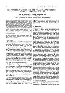
Fig. 1. Left: different ways of organizing a set of grocery objects on shelves according to varying user preferences. Right: our approach enables a service robot to tidy up objects by predicting and following such subjective preferences. We predict pairwise preferences between objects with respect to placing them on the same shelf. We then assign objects to different shelves by maximally satisfying these preferences.

arranging toys in different boxes and grocery items on shelves, as well as a real-robot experiment. For training, we collected preferences from over 1,200 users through different surveys. This paper incorporates the approach and initial results from our previous conference publication [2], and extends our work in the following ways: i) we present a more thorough review of related work, ii) we present a new extension of our approach for inferring the preferences of new users in an efficient manner, and iii) we conduct a more extensive experimental evaluation of all aspects of our method, presenting new results and insights. II. R ELATED W ORK Equipping service robots with the knowledge and skills needed to attend to complex chores in domestic environments has been the aim of researchers for years. Indeed, recent advances in perception, manipulation, planning, and control have enabled robots to perform a variety of chores that range from cleaning and tidying up to folding laundry [13, 17, 32, 43]. However, as highlighted by a number of researchers, service robots should also be able to attend to such tasks in a manner that corresponds to the personal preferences of end users [5, 7, 10, 15, 38, 40, 46]. For example, the results of Pantofaru et al. show that people exhibit strong feelings with respect to robots organizing personal items, suggesting the need for the robot to ask humans to make decisions about where to store them [38]. In this work, we present a novel approach by which robots can discover patterns in organizing objects from a corpus of user preferences in order to achieve preferred object arrangements when tidying up for a specific user. This allows a robot to predict the preferred location (e.g., a specific shelf) to store an object by observing how the user has previously arranged other objects in the same environment. Several researchers have leveraged the fact that our environments are rich with cues that can assist robots in various tasks that require reasoning about objects and their locations. For example, different works have addressed object classification or predicting the locations of objects using typical 3D structures in indoor environments or object-object relations such as co-occurrences in a scene [3, 21, 28, 29, 34]. However, our work is concerned with learning pairwise object preferences to compute preferred arrangements when tidying up. In the remainder of this section, we discuss prior work in

the literature that is most relevant to the problem we address and the techniques we present. a) Learning Object Arrangements and Placements: Recently, Schuster et al. presented an approach for distinguishing clutter from clutter-free areas in domestic environments so that a robot can reason about suitable surfaces for placing objects [45]. Related to that, the work of Jiang et al. targets learning physically stable and semantically preferred poses for placing objects given the 3D geometry of the scene [20]. Joho et al. developed a novel hierarchical nonparametric Bayesian model for learning scenes consisting of different object constellations [22]. Their method can be used to sample missing objects and their poses to complete partial scenes based on previously seen constellations. Other approaches have targeted synthesising artificial 3D object arrangements that respect constraints like physical stability or that are semantically plausible [14, 55]. We view such works as complimentary to ours, as we address the problem of learning preferred groupings of objects in different containers (e.g., shelves) for the purpose of tidying up. After predicting the preferred container for a specific object, our approach assumes that the robot is equipped with a suitable technique to compute a valid placement or pose of the object in that location. Moreover, as we explicitly consider sorting objects when tidying up, we do not reason about object affordances associated with various human poses and activities in the scene (e.g., cooking, working at a desk, etc) when computing arrangements, as in the work of Jiang et al. and Savva et al. [19, 42]. Related to our work, previous approaches have addressed learning organizational patterns from surveys conducted with different users. Schuster et al. presented an approach for predicting the location for storing different objects (e.g., cupboard, drawer, fridge, etc) based on other objects observed in the environment [44]. They consider different features that capture object-related properties (e.g., the purpose of an object or its semantic similarity to other objects) and train classifiers that predict the location at which an object should be stored. Similarly, Cha et al. explored using different features describing both objects and users to train classifiers for predicting object locations in user homes [7]. Similar to Schuster et al., we also make use of a similarity measure

based on hierarchies mined from the Web and use it for making predictions for objects for which we have no training data. However, in contrast to these works, our approach learns latent organizational patterns across different users in a collaborative manner and without the need for designing features that describe objects or users. Recently, Toris et al. presented an approach to learn placing locations of objects based on crowdsourcing data from many users [51]. Their approach allows for learning multiple hypotheses for placing the same object, and for reasoning about the most likely frame of reference when learning the target poses. They consider different pick-and-place tasks such as setting a table or putting away dirty dishes, where the aim is to infer the final object configuration at the goal. Our approach is also able to capture multiple modes with respect to the preferred location for placing a certain object. In contrast to Toris et al., we explicitly target learning patterns in user preferences with respect to sorting objects in different containers. Moreover, in contrast to the above works, our method allows the robot to adapt to the available number of containers in a certain environment to sort the objects while satisfying the user’s preferences as much as possible. Note that in this work, we assume the robot is equipped with a map of the environment where relevant containers are already identified. Previous work has focused on constructing such semantic maps that are useful for robots when planning to solve complex household tasks [37, 52, 57]. b) Service Robots Leveraging the Web: Recently, several researches have leveraged the Web as a useful source of information for assisting service robots in different tasks [24, 49]. To cope with objects that are not in the robot’s database, our method combines collaborative filtering with a mixture of experts approach based on object hierarchies we mine from online stores. This allows us to compute the semantic similarity of a new object to previously known objects to compensate for missing user ratings. The work by Schuster et al. has also utilized such similarity measures as features when training classifiers for predicting locations for storing objects [44]. Pangercic et al. also leverage information from online stores but in the context of object detection [36]. Kaiser et al. recently presented an approach for mining texts obtained from the Web to extract common sense knowledge and object locations for planning tasks in domestic environments [23]. Moreover, Nyga et al. presented an ensemble approach where different perception techniques are combined in the context of detecting everyday objects [34]. c) Collaborative Filtering: We predict user preferences for organizing objects based on the framework of collaborative filtering, a successful paradigm from the data mining community for making personalized user recommendations of products [4, 6, 26, 27, 41]. Such techniques are known for their scalability and suitability for life-long learning settings, where the quality of the predictions made by the recommender system improves with more users providing their ratings. Outside the realm of customers and products, factorizationbased collaborative filtering has recently been successfully applied to other domains including action-recognition in

videos [30] and predicting drug-target interactions [48]. Recently, Matikainen et al. combined a recommender system with a multi-armed bandit formulation for suggesting good floor coverage strategies to a vacuum-cleaning robot by modeling different room layouts as users [31]. To the best of our knowledge, we believe we are the first work to use collaborative filtering for predicting personalized user preferences in the context of service robotics. d) Crowdsourcing for Robotics: To learn different user preferences, we collect data from many non-expert users using a crowdsourcing platform. Prior work has also leveraged crowdsourcing for data labeling or as an efficient platform for transferring human knowledge to robots, e.g., [11, 25]. For example, Sorokin et al. utilized crowdsourcing to teach robots how to grasp new objects [47]. Moreover, several researchers have used crowdsourcing to facilitate learning manipulation tasks from large numbers of human demonstrations [9, 39, 50, 51]. In the context of learning user preferences, Jain et al. recently presented a new crowdsourcing platform where nonexperts can label segments in robot trajectories as desirable or not [18]. This is then used to learn a cost function for planning preferred robot trajectories in different indoor environments. III. C OLLABORATIVE F ILTERING FOR P REDICTING PAIRWISE O BJECT P REFERENCES Our goal is to enable a service robot to reason about the preferred way to sort a set of objects into containers when tidying up in the environment of a specific user. To achieve this, we aim at predicting the preferences of the user with respect to grouping different objects together. As the types of objects (e.g., grocery items) and number of containers (e.g., shelves) typically vary across environments, we aim to learn user preferences for object-object combinations, rather than directly learning an association between an object and a specific container. The problem of predicting an object-object preference for a user closely resembles that of suggesting products to customers based on their tastes. This problem is widely addressed by employing recommender systems, commonly used by websites and online stores such as Amazon and Netflix. The key idea there is to learn to make recommendations based on the purchasing histories of different users collaboratively. In the same spirit of reasoning about products and users, our method relates pairs of objects to users. We predict a user preference, or rating, for an object-pair based on two sources of information: i) known preferences of the user, e.g., how the user has previously organized other objects, and ii) how other users have organized these objects in their environments. A. Problem Formulation More formally, let O = {o1 , o2 , . . . , oO } be a set of objects, each belonging to a known class, e.g., book, coffee, stapler, etc. Accordingly, we define P = {p1 , p2 , . . . , pM } as the set of all pairs of objects from O. We assume to have a finite number of containers C = {c1 , c2 , . . . , cC }, which the robot can use to organize the objects, e.g., shelves, drawers, boxes, etc. We model each container as a set which could be ∅ or could

P (pairs)

u1 u2  p1  * r12 p2   r21 r22     *  . .. pi  .  ..      pM rM 1 *

U (users) uj

*

... ... ..

. rij

..

where µ is a global bias term, bi is the bias of the pair pi , and bj is the bias of user uj . We compute µ as the mean rating over all users and object-pairs in R, i.e.,

uN

.

...



 r2N      *  ..   .       rM N

M 1 XX µ= rij . R i=1

Fig. 2. The ratings matrix R. Each entry rij corresponds to the rating of a user uj for an object-pair pi = {ok , ol }, a value between 0 and 1 denoting whether the two objects should be placed in the same container or not. Our goal is to predict the missing ratings denoted by * and compute a partitioning of the objects in different containers that satisfies the user preferences.

contain a subset of O. Given a set of users U = {u1 , . . . , uN }, we assign a rating rij to a pair pi = {ol , ok } to denote the preference of user uj for placing ol and ok in the same container. Each rating takes a value between 0 and 1, where 0 means that the user prefers to place the objects of the corresponding pair into separate containers, and 1 means that the user prefers placing them together. For convenience, we use r(ol , ok ) to denote the rating for the pair consisting of objects ol and ok when the user is clear from the context. We can now construct a ratings matrix R of size M × N , where the rows correspond to the elements in P and the columns to the users, see Figure 2. We use R to denote the number of known ratings in R. Note that typically, R  M N , i.e., R is missing most of its entries. This is due to the fact that each user typically “rates” only a small subset of object-pairs. In this work, we denote the set of indices of object-pairs that have been rated by user uj by Ij ⊆ {1, . . . , M }. Analogously, Ji ⊆ {1, . . . , N } is the set of indices of users who have rated object-pair pi . Given a set of objects O0 ⊆ O that the robot has to sort for a specific user uj , and the set of containers C available for the robot to complete this task, our goal is to: i) predict the unknown preference rˆij of the user for each of the objectpairs P 0 over O0 and, accordingly, ii) assign each object to a specific container such that the user’s preferences are maximally satisfied. B. Collaborative Learning of User Preferences We aim to discover latent patterns in the ratings matrix R that enable us to make predictions about the preferences of users. For this, we take from factorization-based collaborative filtering [26, 27]. First, we decompose R into a bias matrix B and a residual ratings matrix R: R = B + R.

The bias bj describes how high or low a certain user uj tends to rate object-pairs compared to the average user. Similarly, bi captures the tendency of a pair pi to receive high or low ratings. For example, the pair {salt, pepper} tends to receive generally high ratings compared to the pair {candy, vinegar}. After removing the bias, the residual ratings matrix R captures the fine, subjective user preferences that we aim to learn by factorizing the matrix to uncover latent patterns. Due to the large amount of missing ratings in R, it is infeasible to apply classical factorization techniques such as singular value decomposition. Instead, we learn a data-driven factorization based only on the known entries in R. This approach has been shown to lead to better results in matrix completion or factorization problems compared to imputation of the missing values [6, 26]. We express R as the product of an objectpair factors matrix ST , and a user factors matrix T of sizes M × K and K × N , respectively. Each column si of S is a K-dimensional factors vector corresponding to an objectpair pi . Similarly, each column tj in T is a K-dimensional factors vector associated with a user uj . We compute the residual rating rij as the dot product of the factor vectors for object-pair pi and user uj , i.e., rij = sTi · tj .

(4)

The vectors s and t are low-dimensional projections of the pairs and users, respectively, capturing latent characteristics of both. Pairs or users that are close to each other in that space are similar with respect to some property. For example, some users could prefer to group objects together based on their shape, whereas others do so based on their function. Accordingly, our prediction rˆij for the rating of an objectpair pi by a user uj is expressed as rˆij = bij + rij = µ + bi + bj + sTi · tj .

eij = rij − (µ + bi + bj + sTi · tj ).

M X X

(eij )2 +

b∗ ,S,T i=1 j∈J i

(2)

(6)

We jointly learn the biases and factors that minimize the error over all known ratings, i.e.,

(1)

Each entry bij in B is formulated as follows:

(5)

We learn the biases and factor vectors from all available ratings in R by formulating an optimization problem. The goal is to minimize the difference between the observed ratings rij made by users and the predictions rˆij of the system over all known ratings. Let the error associated with rating rij be

b∗ , S, T = argmin bij = µ + bi + bj ,

(3)

j∈Ji

λ 2 (b + b2j + ksi k2 + ktj k2 ), 2 i

(7)

where b∗ denotes all object-pair and user biases and λ is a regularizer. To do so, we use L-BFGS optimization with a random initialization for all variables [33]. At every step of the optimization, we update the value of each variable based on the error gradient with respect to that variable, which we derive from Equation (7). C. Probing and Predicting for New Users After learning the biases and factor vectors for all users and object-pairs as in Section III-B, we can use Equation (5) to predict the requested rating rˆij of a user uj for an objectpair pi that she has not rated before. However, this implies that we have already learned the bias bj and factor vector tj associated with that user. In other words, at least one entry in the j-th column of R should be known. The set of known preferences for a certain user, used for learning her model, are sometimes referred to as probes in the recommender system literature. In this work, we use probing to refer to the process of eliciting knowledge about a new user. 1) Probing: In the context of a tidy-up service robot, we envision two strategies to do so. In the first probing approach, the robot infers some preferences of the user based on how she has previously sorted objects in the containers C in the environment. By detecting the objects it encounters there, the robot can infer the probe rating for a certain object-pair based on whether the two objects are in the same container or not: ( 1, if ol , ok ∈ cm rij = (8) 0, if ol ∈ cm , ok ∈ cn , m 6= n. We do this for all object-pairs that the robot observes in the environment and fill the corresponding entries in the user’s column with the inferred ratings, see Figure 3. In the second probing approach, we rely on actively querying the user about her preferences for a set of objectpairs. For this, we rely on simple, out-of-the-box user interface solutions such as a text interface where the user can provide a rating. Let P be the maximum number of probe ratings for which the robot queries the user. One naive approach is to acquire probes by randomly querying the user about P object-pairs. However, we aim at making accurate predictions with as few probes as possible. Thus, we propose an efficient strategy based on insights into the factorization of Section IIIB. The columns of the matrix S can be seen as a low dimensional projection of the rating matrix capturing the similarities between object-pairs; object-pairs that are close in that space tend to be treated similarly by users. We therefore propose to cluster the columns of S in P groups, randomly select one column as a representative from each cluster, and query the user about the associated object-pair. For clustering, we use k-means with P clusters. In this way, the queries to the users are selected to capture the complete spectrum of preferences. Note that the nature of a collaborative filtering system allows us to continuously add probe ratings for a user in the ratings matrix, either through observations of how objects are organized in the environment, or by active querying as needed.

o4

r(o1 , o2 ) = 1 r(o1 , o3 ) = 1 .. .

o5 c2

o1

o2

o3 c1

r(o3 , o5 ) = 0 r(o4 , o5 ) = 1

Fig. 3. A simple illustration of the probing process by which the robot can infer some preferences for a new user. We set a rating of 0 for a pair of objects that the robot observes to be in different containers, and a rating of 1 for those in the same container. Using these ratings, we can learn a model of the user to predict her preferences for other object-pairs.

This results in a life-long and flexible approach where the robot can continuously update its knowledge about the user. 2) Inferring a New User’s Preferences: After acquiring probes for the new user, we can now append her column to the ratings matrix and learn her biases and factors vector along with those of all object-pairs and other users in the system as in Equation (7). In practice, we can avoid relearning the model for all users and object-pairs known in the system. Note that the computation of the factorization will require more time as the number of known ratings in R increases or for higher values of K. Here, we propose a more efficient technique suitable for inferring a new user’s preferences given a previously learned factorization. After learning with all object-pairs and users in the database, we assume that all object-pair biases bi and factor vectors S are fixed, and can be used to model the preferences of new users. We can then formulate a smaller problem to learn the bias bj and factors vector tj of the new user uj based on the probe ratings we have for this user, i.e., X λ bj , tj = argmin (eij )2 + (b2j + ktj k2 ), 2 bj ,tj i∈I j X = argmin (rij − (µ + bi + bj + sTi · tj ))2 + (9) bj ,tj

i∈Ij

λ 2 (b + ktj k2 ). 2 j Note that, in general, the inclusion of the ratings of a new user in R will affect the biases and factor vectors of the objectpairs. Whereas Equation (7) represents the batch learning problem to update the model for all users and object-pairs, Equation (9) assumes that the object-pair biases and factor vectors have already been learned from a sufficiently-large set of users that is representative of the new user. This can be useful in a lifelong learning scenario where the robot can efficiently make predictions for a new user when solving a tidy-up task. With more knowledge accumulated about the new users, we can update the factorization model and biases for all object-pairs and users in a batch manner. IV. M IXTURE OF E XPERTS FOR P REDICTING P REFERENCES OF U NKNOWN O BJECTS Thus far, we presented how our approach can make predictions for object-pairs that are known to the robot. In this section, we introduce our approach for computing predictions

Expert E1 Canned Foods Vegetables canned corn

Expert E2

Groceries

tomato sauce

canned tuna

Condiments and Dressings

canned corn

pepper

Spices and Herbs

Canned Foods Vegetables

Spices and Herbs

salt

Groceries

tomato sauce

Sea Food

salt

pepper

canned tuna

Fig. 4. Two examples of expert hierarchies used to compute the semantic similarities between object classes. For example, expert E1 on the left assigns a similarity ρ of 0.4 to the pair {canned corn, canned tuna}, whereas E2 on the right assigns a similarity of 0.33 to the same pair, see Equation (10).

for an object-pair that no user has rated before, for example when the robot is presented with an object o∗ that is not in O. There, we cannot rely on standard collaborative filtering since we have not learned the similarity of the pair (through its factors vector) to others in P. Our idea is to leverage the known ratings in R as well as prior information about object similarities that we mine from the internet. The latter consists of object hierarchies provided by popular websites, including online supermarkets, stores, dictionaries, etc. Figure 4 illustrates parts of two example experts for a grocery scenario. Formally, rather than relying on one source of information, we adopt a mixture of experts approach where each expert Ei makes use of a mined hierarchy that provides information about similarities between different objects. The idea is to query the expert about the unknown object o∗ and retrieve all the object-pair preferences related to it. The hierarchy is a graph or a tree where a node is an object and an edge represents an “is-a” relation. When the robot is presented with a set of objects to organize that includes a new object o∗ , we first ignore object-pairs involving o∗ and follow our standard collaborative filtering approach to estimate preferences for all other object-pairs, i.e., Equation (5). To make predictions for object-pairs related to the new object, we compute the similarity ρ of o∗ to other objects using the hierarchy graph of the expert. For that, we employ the wup similarity [54], a measure between 0 and 1 used to find semantic similarities between concepts ρlk =

depth(LCA(ol , ok )) , 0.5(depth(ol ) + depth(ok ))

(10)

where depth is the depth of a node, and LCA denotes the lowest common ancestor. In the example of expert E1 in Figure 4-left, the lowest common ancestor of canned corn and canned tuna is Canned Foods. Their wup similarity based on E1 and E2 (Figure 4-right) is 0.4 and 0.33, respectively. Note that in general, multiple paths could exist between two object classes in the same expert hierarchy. For example, coffee could be listed under both Beverages and Breakfast Foods. In such cases, we take the path (LCA) that results in the highest wup measure for the queried pair. Given this similarity measure, our idea is to use the known ratings of objects similar to o∗ in order to predict the ratings related to it. For example, if salt is the new object, we can predict a rating for {salt, coffee} by using the rating of

{pepper , coffee} and the similarity of salt to pepper . We compute the expert rating rˆEi (o∗ , ok ) for the pair {o∗ , ok } as the sum of a baseline rating, taken as the similarity ρ∗k , and a weighted mean of the residual ratings for similar pairs, i.e.,

rˆEi (o∗ , ok ) = ρ∗k + η1

X

ρ∗l (r(ol , ok ) − ρlk ),

(11)

l∈L

P where η1 = 1/ l∈L ρ∗l is a normalizer, and L is the set of object indices such that the user’s rating of pair {ol , ok } is known. In other words, we rely on previous preferences of the user (r(ol , ok )) combined with the similarity measure extracted from the expert. The expert hierarchy captures one strategy for organizing the objects by their similarity. If this perfectly matches the preferences of the user, then the sum in Equation (11) will be zero, and we simply take the expert’s baseline ρ∗k when predicting the missing rating. Otherwise, we correct the baseline based on how much the similarity measure deviates from the known ratings of the user. Accordingly, each of our experts predicts a rating using its associated hierarchy. We compute a final prediction rˆE∗ as a combined estimate of all the expert ratings: rˆE∗ (o∗ , ok ) = η2

X

wi rˆEi (o∗ , ok ),

(12)

i

where wi ∈ [0, 1] represents the confidence P of Ei , E∗ denotes the mixture of experts, and η2 = 1/ i wi is a normalizer. We compute the confidence of expert Ei as wi = exp(−ei ), where ei is the mean error in the expert predictions when performing a leave-one-out cross-validation on the known ratings of the user as in Equation (11). We set this score to zero if it is below a threshold, which we empirically set to 0.6 in our work. Moreover, we disregard the rating of an expert if o∗ cannot be found in its hierarchy, or if all associated similarities ρ∗l to any relevant object ol are smaller than 0.4. Note that in general, both objects in a new pair could have been previously encountered by the robot separately, but no rating is known for them together. When retrieving similar pairs to the new object-pair, we consider the similarities of both objects in the pair to other objects. For example, we can predict the rating of {sugar , coffee} by considering the ratings of both {flour , coffee} and {sugar , tea}.

c1

c2

o2

o5

c3 o7

o3

o8

o1

o4

o6

implement a self-tuning heuristic which sets the number of clusters C 0 based on the location of the biggest eigen-gap from the decomposition of L, which typically indicates a reliable way to partition the graph based on the similarities of its nodes. A good estimate for this is the number of eigenvalues of L that are approximately zero [53, 56]. If there exist less containers in the environment than this estimate, we use all C containers for partitioning the objects. VI. E XPERIMENTAL E VALUATION

o6

o7

o4

o5

o8 c3 c2

o1

o2

o3 c1

Fig. 5. Top: a graph depicting the relations between objects. Each node corresponds to an object, and the weights (different edge thickness) correspond to the pairwise ratings. We partition the graph into subgraphs using spectral clustering. Bottom: we assign objects in the same subgraph to the same container.

V. G ROUPING O BJECTS BASED ON P REDICTED P REFERENCES Now that it is possible to compute pairwise object preferences about known or unknown objects, we aim to sort the objects into different containers. In general, finding a partitioning of objects such that all pairwise constraints are satisfied is a non-trivial task. For example, the user can have a high preference for {pasta, rice} and for {pasta, tomato sauce}, but a low preference for {rice, tomato sauce}. Therefore, we aim at satisfying as many of the preference constraints as possible when grouping the objects into C 0 ≤ C containers, where C is the total number of containers the robot can use. First, we construct a weighted graph where the nodes represent the objects, and each edge weight is the rating of the corresponding object-pair, see Figure 5. We formulate the subdivision of objects into C 0 containers as a problem of partitioning of the graph into C 0 subgraphs such that the cut (the sum of the weights between the subgraphs) over all pairs of subgraphs is minimized. This is called the minimum k-cut problem [16]. Unfortunately, finding the optimal partitioning of the graph into C 0 ≤ C subgraphs is NP-hard. In practice, we efficiently solve this problem by using a spectral clustering approach [8]. The main idea is to partition the graph based on the eigenvectors of its Laplacian matrix, L, as this captures the underlying connectivity of the graph. Let V be the matrix whose columns are the first C 0 eigenvectors of L. We represent each object by a row of the matrix V , i.e., a C 0 -dimensional point, and apply kmeans clustering using C 0 clusters to get a final partitioning of the objects. To estimate the best number of clusters, we

In this section, we present the experimental evaluation of our approach by testing it on two tidy-up scenarios. We first demonstrate different aspects of our approach for a simple scenario of organizing toys in boxes based on a small dataset with 15 survey participants. In the second scenario, we address sorting grocery items on shelves, and provide an extensive evaluation based on ratings we collected from over 1,200 users using crowdsourcing. We demonstrate that: i) users indeed have different preferences with respect to sorting objects when tidying up, ii) our approach can accurately predict personal user preferences for organizing objects (Section III-B), iii) we are able to efficiently and accurately learn a model for a new user’s preferences based on previous training users (Section III-C), iv) our mixture of experts approach enables making reasonable predictions for previously unknown objects (Section IV), v) our approach is suitable for life-long learning of user preferences, improving with more knowledge about different users, vi) our object partitioning approach based on spectral clustering can handle conflicting pairwise preferences and is flexible with respect to the number of available containers (Section V), and vii) our approach is applicable on a real tidy-up robot scenario. In the following experiments, we evaluate our approach using two different methods for acquiring probe ratings, and compare our results to different baselines. For that, we use the following notation: • CF refers to our collaborative filtering approach for learning user preferences, as described in Section III-B. When selecting probes to learn for a new user, we do so by clustering the object-pairs based on their learned factor vectors in order to query the user for a range of preferences, see Section III-C.1. • CF-rand selects probes randomly when learning for a new user and then uses our collaborative filtering approach to make predictions as in Section III-B. 0 • CF-rand selects probes randomly and learns the preferences of a new user based on the object-pair biases and factor vectors learned from previous users as in Section III-C.2. • Baseline-I uses our probing approach as in CF, and then predicts each unknown pair rating as the mean rating over all users who rated it. • Baseline-II selects probes randomly and then predicts each unknown pair rating as the mean rating over all users. In all experiments, unless stated otherwise, we set the number of factor dimensions to K = 3 and the regularizer

1

U1 0

U2 −1

−2

−2

−1

0

1

Fig. 6. Left: we considered a scenario of organizing toys in boxes. Right: a visualization of user tastes with respect to organizing toys, where we plot the user factor vectors projected to the first two dimensions. For example, the cluster U1 corresponds to users who grouped all building blocks together in one box. Cluster U2 corresponds to users who separated building blocks into standard bricks, car-shaped blocks, and miscellaneous.

to λ = 0.01. As part of our implementation of Equation (7) and Equation (9), we rely on the L-BFGS implementation by Okazaki and Nocedal [35]. Note that in our work, we assume that the robot is equipped with suitable techniques for recognizing the objects of interest. In our experiments, we relied on fiducial markers attached to the objects, and also implemented a classifier that recognizes grocery items by matching visual features extracted from the scene to a database of product images. A. Task 1: Organizing Toys In this experiment, we asked 15 people to sort 26 different toys in boxes, see Figure 6-left. This included some plush toys, action figures, a ball, cars, a flashlight, books, as well as different building blocks. Each participant could use up to six boxes to sort the toys. Overall, four people used four boxes, seven people used five boxes, and four people used all six available boxes to sort the toys. We collected these results in a ratings matrix with 15 user columns and 325 rows representing all pairs of toys. Each entry in a user’s column is based on whether the user placed the corresponding objects in the same box or not, see Section III-C.1. For a fine quantification, we used these ratings to bootstrap a larger ratings matrix representing a noisy version of the preferences with 750 users. For this, we randomly selected 78 ratings out of 325 from each column. We repeated this operation 50 times for each user and constructed a ratings matrix of size 325×750 where 76% of the ratings are missing. As a first test, we computed a factorization of the ratings matrix as described in Section III-B. Figure 6-right shows the user factors T projected to the first two dimensions, giving a visualization of the user tastes. For example, the cluster of factors labeled U1 corresponds to users who grouped all building blocks together in one box. 1) Predicting User Preferences for Pairs of Toys: We evaluated our approach for predicting the preferences of the 15 participants by using the partial ratings in the matrix we constructed above. For each of the participants, we queried for the ratings of P probes. We hid all other ratings from the user’s column and predicted them using the ratings matrix and our approach. We rounded each prediction to the nearest integer on the rating scale [0,1] and compared it to the ground

truth ratings. We evaluated our results by computing the precision, recall, and F-score of our predictions with respect to the two rating classes: no (r = 0), and yes (r = 1). We set the number of probes to P = 50, 100, . . . , 300 known ratings, and repeated the experiment 20 times for each value, selecting different probes in each run. The mean F-scores of both rating classes, averaged over all runs are shown in Figure 7-top. Both collaborative filtering techniques outperform baselines I and II. On average, CF and CF-rand maintain an F-score around 0.98 over all predicted pair ratings. On the other hand, Baseline-I and Baseline-II achieve an F-score of 0.89 on average. By employing the same strategy for all users, these baselines are only able to make good predictions for object-pairs that have a unimodal rating distribution over all users, and cannot generalize to multiple tastes for the same object-pair. 2) Sorting Toys into Boxes: We evaluated our approach for grouping toys into different boxes based on the predicted ratings in the previous experiment. For each user, we partitioned the objects into boxes based on the probed and predicted ratings as described in Section V, and compared that to the original arrangement. We computed the success rate, i.e., the percentage of cases where we achieve the same number and content of boxes, see Figure 7-bottom. Our approach has a success rate of 80% at P = 300. As expected, the performance improves with the number of known probe ratings. On the other hand, even with P = 300 known ratings, Baseline-I and Baseline-II have a success rate of only 56% and 58%. Whereas CF-rand achieves a success rate of 82% at P = 300, it requires at least 200 known probe ratings on average to achieve success over 50%. On the other hand, CF achieves a success rate of 55% with only 100 known probe ratings. The probes chosen by our approach capture a more useful range of object-pairs based on the distribution of their factor vectors, which is precious information to distinguish a user’s taste. 3) Predicting Preferences for New Objects: We evaluated the ability of our approach to make predictions for objectpairs that no user has rated before (Section IV). For each of the 26 toys, we removed all ratings related to that toy from the ratings of the 15 participants. We predicted those pairs using a mixture of three experts and the known ratings for the

TABLE I T HE DISTRIBUTION OF RATINGS FOR THE GROCERIES SCENARIO

Mean F-score

1

OBTAINED THROUGH CROWDSOURCING . OVERALL , WE GATHERED 37,597 RATINGS ABOUT 179 OBJECT- PAIRS FROM 1,284 USERS . F OR EACH OBJECT- PAIR , USERS INDICATED WHETHER THEY WOULD PLACE THE TWO OBJECTS ON THE SAME SHELF OR NOT.

0.9

0.8 CF Baseline-I

CF-rand Baseline-II

0.7

Rating Percentage 50

100

150

200

250

no (r = 0) 47.9%

Rating Classes maybe yes (r = 0.5) (r = 1) 29.2% 22.9%

300

Success rate for grouping toys (%)

Number of probes, P

CF Baseline-I

100

objects together on the same shelf. Each user could answer with no, maybe, or yes, which we translated to ratings of 0, 0.5, and 1, respectively. We aggregated the answers into a ratings matrix R of size 179×1,284. Each of the user columns contains between 28 and 36 known ratings, and each of the 179 object-pairs was rated between 81 to 526 times. Overall, only around 16% of the matrix is filled with ratings, with the ratings distributed as in Table I. Due to the three possible ratings and the noise inherent to crowdsourcing surveys, the ratings we obtained were largely multi-modal, see Figure 8 for some examples.

CF-rand Baseline-II

80 60 40 20 50

100

150

200

250

300

Number of probes, P Fig. 7. Top: the mean F-score of the predictions of our approach (CF) in the toys scenario for different numbers of known probe ratings. We achieve an F-score of 0.98-0.99 on average over all predicted ratings. CF-rand selects probes randomly and then uses our approach for predicting. It is able to achieve an F-score of 0.98. On the other hand, baselines I and II are unable to adapt to multimodal user preferences. Bottom: the percentage of times our approach is able to predict the correct arrangement of boxes for sorting different toys. We outperform both baselines and improve with more probe ratings as expected, reaching a success rate of 80%. By selecting probes based on object-pair factor vectors, we are able to achieve higher success rates with less probes compared to CF-rand.

remaining toys. We evaluated the F-scores of our predictions as before by averaging over both no and yes ratings. We based our experts on the hierarchy of an online toy store (toysrus.com), appended with three different hierarchies for sorting the building blocks (by size, color, or function). The expert hierarchies contained between 165-178 nodes. For one of the toys (flash light), our approach failed to make predictions since the experts found no similarities to other toys in their hierarchy. For all other toys, we achieved an average F-score of 0.91 and predicted the correct box to place a new toy 83% of the time. B. Task 2: Organizing Groceries In this scenario, we considered the problem of organizing different grocery items on shelves. We collected data from over 1,200 users using a crowdsourcing service [1], where we considered a set of 22 common grocery item types, e.g., cans of beans, flour, tea, etc. We asked each user about her preferences for a subset of pairs related to these objects. For each pair, we asked the user if she would place the two

1) Predicting User Preferences for Pairs of Grocery Items: We show that our approach is able to accurately predict user ratings of object-pairs using the data we gathered from crowdsourcing. For this, we tested our approach through 50 runs of cross-validation. In each run, we selected 50 user columns from R uniformly at random, and queried them with P of their known ratings. We hid the remaining ratings from the matrix and predicted them using our approach. We rounded each prediction to the closest rating (no, maybe, yes) and evaluated our results by computing the precision, recall, and F-score. Additionally, we compared the predictions of our approach (CF) to CF-rand, Baseline-I, and Baseline-II described above. The average F-scores over all runs and rating classes are shown in Figure 9-top for P = 4, 8, . . . , 20. Both collaborative filtering approaches outperform the baseline approaches, reaching a mean F-score of 0.63 at P = 20 known probe ratings. Baseline-I and Baseline-II are only able to achieve an F-score of 0.45 by using the same rating of a pair for all users. Note that by employing our probing strategy, our technique is able to achieve an F-score of 0.6 with only 8 known probe ratings. On the other hand, CF-rand needs to query a user for the ratings of at least 12 object-pairs on average to achieve the same performance. For a closer look at the performance with respect to the three rating classes, we select the results at P = 12 and show the per-class precision, recall, and F-score values for both CF and Baseline-I in Figure 10-top. Note that the baseline achieves its highest recall value for the maybe class since it uses the mean rating received by a specific object-pair to predict its rating for new users. On the other hand, we are able to achieve a similar recall (0.63) for the maybe class, as well as higher recall values for the no and yes classes despite the large degree of noise and the variance in people preferences

100 80 60 40 20 0

{tomato sauce, cans of corn}

%

%

{bread , jam}

100 80 60 40 20 0

no maybe yes

no maybe yes

no maybe yes

{olive oil , pasta}

{coffee, tea}

{candy, salt}

no maybe yes

100 80 60 40 20 0

%

100 80 60 40 20 0

%

%

%

{flour , spices} 100 80 60 40 20 0

no maybe yes

100 80 60 40 20 0 no maybe yes

Fig. 8. Example distributions of the ratings given by users for different object-pairs. Each user could answer with no (r = 0), maybe (r = 0.5), or yes (r = 1) to indicate the preference for placing the two objects on the same shelf. The three possible rating classes, as well as the noise inherent to crowdsourcing surveys, resulted in multi-modal taste distributions. This highlights the difficulty of manually designing rules to guide the robot when sorting objects into different containers.

in the training data. Our approach is able to achieve higher F-scores over all rating classes compared to the baseline. Out of the three classes, we typically achieved better scores for predicting the no class compared to maybe or yes. This is expected due to the distribution of the training ratings we gathered from the crowdsourcing data, see Table I. Additionally, we computed the prediction error (Equation (6)) averaged over all experimental runs for each value of P , see Figure 9-bottom. The baselines are unable to cope with the different modes of user preferences, and consistently result in a prediction error of around 0.27 irrespective of the number of probes. On the other hand, the mean prediction error using CF and CF-rand drops from 0.24 to 0.18 and from 0.25 to 0.19 as P increases from 4 to 20, respectively. Note that, using our probing technique, we are able to achieve a lower error with fewer probes compared to CF-rand. This illustrates the importance of selecting more intelligent queries for users to learn their preferences. For a closer inspection of the prediction error, Figure 10-bottom shows the distribution of the error for our approach and Baseline-I given P = 12 probes. Our approach achieves an error of 0 for 64.62% of the predictions we make, compared to 49.78% only for BaselineI. Moreover, Baseline-I results in an absolute error of 0.5 (confusing no/yes with maybe) for 47.60% of the predictions, compared to 32.88% only for our approach. Finally, our approach and the baseline result in a prediction error of 1.0 (misclassifying no as yes or vice versa) for only 2.49% and 2.62% of the predictions, respectively. 2) The Effect of the Number of Latent Dimensions: In this experiment, we investigated the effect of varying the number of latent dimensions K used when learning the factorization of R on the quality of the learned model. We repeated the experiment in Section VI-B.1 for K = 3, 6, 9, 15. For each setting of K, we conducted 50 runs where, in each run, we

selected 50 random user columns, queried them for P random probe ratings, and learned the factorization in Section III-B to predict the remaining ratings. As in the previous experiment, we evaluated the quality of predicting the unknown ratings by computing the average F-score for the no, maybe, and yes classes. Additionally, we computed the root mean square error (RMSE) for reconstructing the known ratings in R used in training, i.e., s RMSE =

2 1 XX rij − (µ + bi + bj + sTi · tj ) . R i j∈Ji

The results are shown in Figure 11. When using larger values of K, we are able to reconstruct the known ratings in R with lower RMSE values. This is expected since we are computing a more accurate approximation of R when factorizing it into higher-dimensional matrices (S and T), thus capturing finer details in user preferences. However, this results in over-fitting (lower F-scores) when predicting unknown ratings, especially for lower values of P . In other words, for higher values of K, we need more probes per user when predicting unknown ratings, since we need to learn more factors for each user and object-pair. In general, the more known ratings we have in the user columns, the more sophisticated are the models that we can afford to learn. Furthermore, we found interesting similarities between object-pairs when inspecting their learned biases and factor vectors. For example (for K = 3), users tend to rate {coffee, honey} similarly to {tea, sugar } based on the similarity of their factor vectors. Also, the closest pairs to {pasta, tomato sauce} included {pancakes, maple syrup} and {cereal , honey}, suggesting that people often consider whether objects can be used together or not. With respect to the biases (bi ) learned, object-pairs with the largest

CF Baseline-I

0.7

CF-rand Baseline-II

F-score

Baseline-I 0.6

CF

0.5

0.4

maybe

yes

Precision

0.71

0.34

0.79

Recall

0.52

0.69

0.19

F-score

0.60

0.46

0.31

Precision

0.80

0.45

0.72

Recall

0.72

0.63

0.49

F-score

0.76

0.53

0.58

10

15

20

Number of probes, P

CF Baseline-I

0.35

CF-rand Baseline-II

0.3 0.25

Percentage of predictions

80 5

Mean prediction error

no

CF Baseline-I 60

40

20

0

0.2

0

0.5

1.0

Absolute prediction error 0.15 5

10

15

20

Number of probes, P

Fig. 9. Results for the scenario of organizing grocery items on different shelves. Top: the mean F-score of our predictions averaged over all rating classes no, maybe, and yes. Despite the large degree of multi-modality and noise in the user preferences we collected through crowdsourcing, our approach (CF) is able to achieve an F-score of 0.63 with 20 known probes and to outperform the baselines. Moreover, our performance improves with more knowledge about user preferences as expected. Bottom: the mean prediction error for different numbers of probes, P . The baselines are unable to cope with different modes of user preferences. They consistently result in a prediction error of around 0.27 irrespective of the number of probes. On the other hand, the mean prediction error using CF 0.24 to 0.18 as P increases from 4 to 20. Using our probing technique, we are able to achieve a lower error with fewer probes compared to CF-rand.

biases (rated above average) included {pepper , spices}, {pasta, rice} and {cans of corn, cans of beans}. Examples of object-pairs with the lowest biases (rated below average) included {candy, olive oil }, {cereal , vinegar }, and {cans of beans, cereals}. On the other hand, object-pairs like {cans of corn, pasta} and {pancakes, honey} had a bias of almost 0. 3) Learning of New User Preferences: In this experiment, we show that our approach is able to learn the preferences of new users based on the object-pair biases and factor vectors learned from previous users, see Section III-C.2. We conducted an experiment similar to that in Section VI-B.1 using a random probing strategy. However, we first learned the biases bi and factor vectors S using rating matrices R100 , R250 , . . . , R1000 , corresponding to 100, 250, . . . , 1000 training users, respectively (Equation (7)). We then used this model to compute the biases bj and factor vectors T for a set of 100 (different) test users (Equation (9)) and predict their missing ratings. As before, we repeated this

Fig. 10. Top: the detailed evaluation for the groceries scenario with P = 12 probes. Our approach results in higher F-scores across all rating classes compared to the baseline. Figure 9-top shows the mean F-score for different values of P . Bottom: the detailed distribution of the prediction errors using P = 12 probes, see Figure 9-bottom for the mean error for different values of P .

experiment for different values P of known probe ratings for the test users. The prediction F-score averaged over 50 runs is shown in Figure 12-top. As expected, the performance improves given more training users for learning the bi ’s and S, converging to the performance when training with all user columns (compare to CF-rand in Figure 9-top). This validates that, given enough users in the robot’s database, we can decouple learning a projection for the object-pairs from the problem of learning the new users’ biases and factor vectors. Moreover, we compared the predictions using this approach (CF-rand0 ) to the standard batch approach that first appends the 100 new user columns to the training matrix and learns all biases and factor vectors collaboratively (CF-rand). The prediction error, averaged over the 50 runs, is shown in Figure 12-bottom for P = 12 probe ratings. As expected, the error for both approaches drops given more training users, converging to 0.20 for R750 and R1000 , i.e., approaching the performance when training with the full R (compare to CF-rand in Figure 9-bottom for P = 12). Furthermore, with smaller training matrices, we observed a slight advantage in performance for CF-rand0 . In other words, given fewer ratings, it might be advantageous to solve the smaller optimization problem in Equation (9). Probing and Learning for New Users: Using our method, the time for computing the model for one new user (based on a previously-learned factorization) on a consumer-grade notebook was 10-20 ms on average, compared to about 4 s for batch learning with all 1248 user columns (K = 3). To

0.3

0.6 RMSE

F-score

0.2

R100 R500 R1000

0.5

0.1

4

0 3

6

6 9 12 15 Number of latent dimensions, K

R250 R750

8 10 12 14 16 18 20 Number of probes, P

F-score

0.7

K=3

K=9

Mean prediction error

0.3 K = 15

0.6

0.5

CF-rand CF-rand0 0.2

0.1

0 R100 5

10

15

20

Number of probes, P

Fig. 11. We learned different factorizations of the ratings matrix R by varying the number of latent dimensions, K. For each learned model, we evaluated the RMSE when reconstructing the known ratings in R (top), and the F-score for predicting unknown ratings in R given different numbers of probes P for randomly selected user columns (bottom). Learning factors (S and T) with larger dimensionality leads to reconstructing the known ratings in R with a higher fidelity (lower RMSE). However, this comes at the expense of over-fitting to the known ratings for users, leading to lower F-scores with larger K when predicting new ratings given the same number of probes, P .

R250 R500 R750 R1000 Training matrix, RN

Fig. 12. Top: we tested our approach for learning the preferences of new users based on the object-pair biases and factors vectors learned from rating matrices RN of different sizes. The results are shown for predicting with a set of 100 test users based on P random probe ratings each, averaged over 50 runs. The performance improves with more training users as expected, approaching the performance when training with all users, see Figure 9-top for comparison. Given sufficient users in the robot’s database (≥ 750), we can infer the preferences of new users by assuming fixed object-pair biases and factor vectors without loss in prediction accuracy. Bottom: the prediction error given P = 12 probe ratings when inferring the preferences of test users given a previously-learned factorization (CF-rand0 ) compared to batch learning with the training and test users combined (CF-rand). As expected, the error for both approaches drops given more training users, converging to 0.20 for R750 and R1000 , i.e., approaching the performance when training with the full R, see Figure 9-bottom.

demonstrate the applicability of our approach (Section IIIC) in a real-world scenario, we conducted an experiment where we used a Kinect camera to identify a set of objects object-pairs. For this, we defined three experts by mining that we placed on shelves and used the perceived pairwise the hierarchies of the groceries section of three large online ratings as probes for inferring a user’s preference. For stores (amazon.com, walmart.com, target.com). This includes perception, we clustered the perceived point cloud to segment up to 550 different nodes in the object hierarchy. For each the objects, and relied on SIFT features matching using of the 22 grocery objects, we removed ratings related to a database of product images to label each object. We all of its pairs from R, such that the typical collaborative learned the bias and factors vector for the user associated filtering approach cannot make predictions related to that with this scene using the object-pairs model that we learnt object. We used the mixture of experts to predict those ratings with our crowdsourcing data. Accordingly, we predicted using the remaining ratings in each column and the expert the pairwise ratings related to objects that are not in the hierarchies as explained in Section IV. The mean F-score over scene and computed the preferred shelves to place them on. all users for three grocery objects is shown in Figure 14-top, Figure 13 shows an example where the top image shows the where the mixture of experts is denoted by E∗ . We also show camera image of the scene, and the bottom image shows the individual expert results (E1 -E3 ) and their corresponding the corresponding computed shelf arrangement in the rviz baseline predictions (E 0 -E 0 ). The baselines take only the wup 1 3 visualization environment. Due to physical space constraints, similarity of two objects as the rating of the pair but do we assume that each shelf is actually divided into two not consider the ratings of similar pairs made by the same shelves. A video demonstrating how the predicted arrange- user as our approach does. As we can see, the results of ment changes as the configuration on the shelves varies can each individual expert outperform the baseline predictions. be seen at http://www.informatik.uni-freiburg. Note that E∗ is able to overcome the shortcomings of the de/%7Eabdon/task_preferences.html. individual experts, as in the case of rice. There, E1 is unable 4) Predicting Preferences for New Objects: In this experi- to find similarities between rice and any of the rated objects, ment, we demonstrate that our mixture of experts approach whereas E2 and E3 are able to relate it to pasta in their is able to make reasonable predictions for previously unrated hierarchies. For two of the objects (bread and candy), we

1

E10 E1 E20 E2 E30 E3 E∗

F-score

0.8 0.6 0.4 0.2 0 cans of beans

coffee

rice

F-score

0.6 0.5 0.4 0.3

CF - cereal CF - overall 0

Fig. 13. An application of our approach that demonstrates how our predictions for a new user change based on how (probing) objects are arranged on the shelves. Top: the camera image of the scene. To label the objects, we relied on matching SIFT features from a database of images for the used products. Bottom: a visualization of the predicted preferred arrangement of other objects based on the corresponding learned model. Our method is able to infer the user’s preferences by adapting to the perceived arrangement. For example, by moving coffee from the shelf containing tea to the one containing flour , the predicted arrangement separates cake mix and sugar and moves them to different shelves.

were unable to make any predictions, as none of the experts found similarities between them and other rated objects. For all other objects, we achieve an average F-score of 0.61. Predicting Ratings for New Object-Pairs: Furthermore, we applied the same mixture of experts based on the three online stores above to extend our ratings matrix R with rows for object-pairs that no user rated in our crowdsourcing surveys. We created a new ratings matrix R0 of size 214×1284, i.e., with 35 additional object-pair rows. These included pairs related to the new object cake mix , as well as other object combinations. For each user column in the original R, the mixture of experts used already-rated object-pairs to infer ratings for the new pairs. Figure 15 shows examples of rating distributions in the resulting ratings matrix for two objectpairs: {cans of beans, sugar } and {cake mix , flour }. Additionally, for each of them, we show the rating distributions of two of their most similar object-pairs that the experts used when making their predictions. In a later experiment, we use the resulting R0 with this combination of crowdsourcing and expert-generated ratings to train a factorization model for predicting preferred arrangements of survey participants, see Section VI-B.6. 5) Improvement with Number of Users: We conducted an experiment to show that the performance of our approach improves with more users in the system. For each object,

50

CF - olive oil Baseline - overall

100 150 200 250 Number of columns

300

Fig. 14. Top: we predict preferences related to new objects by using a mixture of experts approach. The experts E1 -E3 are based on the hierarchies of three online grocery stores. The mixture of experts E∗ is a merged prediction of all three experts based on their confidence for a specific user. Therefore, it is able to recover if a certain expert cannot find similarities for a new object, as in the case of rice. The baselines E10 -E30 make predictions based only on the semantic wup similarity of two objects without considering the ratings of similar pairs rated by the user, see Section IV. Bottom: the mean F-score for predicting the ratings for a new object vs. the number of training user columns who have rated pairs related to it. As soon as some users have rated pairs related to a new object, our collaborative filtering approach is able to make predictions about it. The performance improves with more users rating pairs related to the object.

we removed from R all columns with ratings related to that object. Over 20 runs, we randomly sampled ten different user columns (test users) from these and hid their ratings for pairs related to the object. We predicted those ratings using our approach (Section III-B) by incrementally adding more columns of other (training) users who rated that object to the ratings matrix in increments of 25. We evaluated the mean F-score for the predictions for the test users. The results (CF - overall) are shown in Figure 14-bottom averaged over 20 different types of objects (those where we had at least 300 user ratings). We also show the improvement with respect to two of the objects individually. The performance of our approach improves steadily with the number of users who rate pairs related to a new object, as opposed to a baseline that updates the mean rating over all users and uses that for predicting. This shows that collaborative filtering is suitable for lifelong and continual learning of user preferences. 6) Assigning Objects to Shelves Based on Pairwise Preferences: The goal of this experiment is to show that our approach is able to group objects into containers to satisfy pairwise preferences, see Section V. We evaluated our

{cans of beans, flour } 100 80 60 40 20 0

no maybe yes

no maybe yes

{flour , sugar }

{pancakes mix , flour }

100 80 60 40 20 0

%

%

%

no maybe yes

100 80 60 40 20 0

no maybe yes

{cake mix , flour } 100 80 60 40 20 0

{cans of tuna, sugar }

%

%

%

{cans of beans, sugar } 100 80 60 40 20 0

no maybe yes

100 80 60 40 20 0 no maybe yes

Fig. 15. The rating distributions depicted in red correspond to example object-pairs that no user had rated in the original crowdsourcing data. We generated those ratings using our mixture of experts approach based on the hierarchies of three online stores. In the case of {cans of beans, sugar }, the experts relied on how each user rated similar object-pairs such as {cans of beans, flour } and {cans of tuna, sugar }. The rating distributions of those pairs (over all user columns who rated them) are depicted in blue on the same row. Similarly, in the case of {cake mix , flour }, the experts relied on the known ratings of {flour , sugar } and {pancake mix , flour }.

100 Percentage of cases (%)

approach in two settings. In the first, we compute the object groupings given ground truth pairwise ratings from users. In the second, we predict the pairwise ratings according to our approach and use those when grouping the objects on different shelves. a) Arrangements Based on Ground Truth Ratings: We conducted a qualitative evaluation of our approach for grouping objects into different containers based on known object-pair preferences. We asked a group of 16 people to provide their ratings (0 or 1) for 55 object-pairs, corresponding to all pairs for a set of 11 objects. For each participant, we then computed an object arrangement allowing our spectral clustering approach to use up to 6 shelves. We showed each participant the shelf arrangement we computed for them in the rviz visualization environment. We asked each of them to indicate whether they think the arrangement represents their preferences or not. They then had the choice to make changes to the arrangement by indicating which objects they would move from one shelf to another. The results are shown in Figure 16. In five out of 16 cases, the participants accepted the arrangements without any modifications. Overall, the participants modified only two objects on average. Even given ground truth object-pair ratings from the users, there are often several inconsistencies in the preferences that can make it challenging for the eigengap heuristic to estimate the best number of shelves to use. Nonetheless, we are able to compute reasonable groupings of objects. Moreover, the nature of our approach allows the robot to observe arrangements given by users in order to modify its knowledge about their preferences and use this when making new predictions in the future. b) Arrangements Based on Predicted Ratings: The goal of this experiment is to evaluate the performance of our

80 60 40 20 0 0

≤1

≤2

≤3

≤4

≤5

Number of objects moved

Fig. 16. In a small survey with 16 participants, we computed groupings of 11 objects based on each participant’s ground truth object-pair ratings. We presented the arrangement to each participant by visualizing it in a 3D visualization environment. Each participant then indicated which objects they would like to move in order to achieve a better arrangement. Despite inconsistencies in the pairwise preferences of the participants, we are able to compute reasonable object groupings that correspond to their preferences. On average, the participants modified the locations of only two objects.

Fig. 17. We asked survey participants to organize different types of grocery objects using up to six shelves in order to test our approach for predicting their preferences.

approach for grouping objects based on predicted objectpair ratings. To collect ground truth data for arrangements, we asked 15 people to organize 17 different grocery items according to their preferences, using up to six shelves, see Figure 17. Four people grouped the items on four shelves, three people used five shelves, and eight people used all six shelves. Figure 1-left shows examples of arrangements produced by the survey participants. We translated these arrangements to user rating columns with 0 or 1 ratings as described in Section IIIC.1. Figure 18 shows the arrangements our method computes for one of the participants (who used four shelves) when given all ground truth object-pair ratings of that participant. Given four or more shelves to use, we are able to reproduce the original object grouping of this user with C 0 = 4 shelves. The figure also shows how our approach adapts by merging some object groups together when given only two or three shelves to sort the objects. Our goal is to evaluate the arrangements we compute for the 15 participants given only partial knowledge of their ratings, and based on a previously-learned model of object-pair biases bi and factor vectors S from training users. To learn the model, we used the ratings matrix R0 described in Section VI-B.4 above, as this covers all object-pairs relevant for the objects in this experiment. For each of the 15 participants, we then simulated removing O random objects from their arrangement, and hid all ratings related to those objects. Using the remaining ratings as probes, we learned the bias bj and factors vector tj of each participant (Section III-C.2), and predicted the missing ratings accordingly. Finally, we used those ratings to compute an object arrangement for each participant, and compared it to their ground truth arrangement. We conducted this experiment for O = 1, 2, 3, . . . , 12, repeating it 100 times for each setting. We evaluated the results by computing an “edit” distance d between the computed and ground truth arrangements. We compute d as the minimum number of objects we need to move from one shelf to another to achieve the correct arrangement, divided by O. This gives a normalized error measure between 0 and 1 capturing the ratio of misplaced objects. The results (averaged over all runs) are shown in Figure 19-top, where we denote our method by CF-rand0 . We compared our results to two baselines. The first is Baseline-II, which predicts the missing object-pair preferences using the mean ratings over all users in R0 and then computes the object groupings using our approach. The second is Baseline-III, which makes no predictions but simply assigns each object to a random shelf. Figure 19-bottom also shows the mean F-score of our approach and Baseline-II averaged over the 0 and 1 rating categories. Our approach outperforms both baselines for O ≤ 10, and results in a mean error from 0.19 to 0.41, and an F-score from 0.80 to 0.78, as O changes from 1 to 10. The model we learned from R0 (noisy crowdsourcing data from 1284 users augmented by ratings from a mixture of experts) is able to accurately predict the preferences of the new 15 survey participants. For the same values of O, Baseline-II achieves a mean error ranging between 0.36 and 0.54, and an F-score of

TABLE II T HE ERROR d IN THE FINAL ARRANGEMENT PRODUCED BY 15 PARTICIPANTS WHEN WE ASKED THEM TO SORT O OBJECTS BY PREDICTING THE PREFERENCES OF USERS THEY DO NOT KNOW.

Number of objects, O 2 4 6 8 10 12

Error in arrangement, d 0.07 ± 0.17 0.27 ± 0.25 0.24 ± 0.22 0.27 ± 0.18 0.33 ± 0.18 0.34 ± 0.17

0.77. As O increases, the error in our predictions increases as expected, since we have less probe ratings based on the remaining objects on the shelves to infer the preferences of a new user. For O > 11, Baseline-II results in less error than our approach when computing arrangements. On the other hand, using a random strategy for assigning objects to shelves (Baseline-III) resulted in an error above 0.72 for all values of O. c) Predictions by Humans: Finally, we conducted a qualitative evaluation to gauge the difficulty of the above task for humans. We asked 15 new participants (who did not take part in the previous surveys) to complete partial arrangements by predicting the preferences of the 15 users above, whom they do not know. Each participant solved six tests. In each test, we manually reconstructed an arrangement from the surveys on the six shelves, then we removed O objects randomly and placed them on a nearby table. We asked each participant to predict the preference of another user by inspecting the arrangement in front of them, and to finish sorting the remaining O objects accordingly. Each participant solved six such cases (O = {2, 4, . . . , 12}), each corresponding to a different user. As before, we computed the error d, the ratio of objects that were placed on wrong shelves. The results are shown in Table II. When presented with two objects to place only, most participants were able to predict the correct shelf for them based on the arrangement of the remaining objects. However, given four to twelve objects, the participants misplaced between one forth to one third of the objects on average. 7) Real Robot Experiments: We conducted an experiment to illustrate the applicability of our approach (Section III-B) on a real tidy-up robot scenario using our PR2 robot platform, see Figure 20-left. We executed 25 experimental runs where the task of the robot was to fetch two objects from the table and return them to their preferred shelves as predicted by our approach. In each run, we arranged 15 random objects on the shelves according to the preferences of a random user from the survey we conducted in Section VI-B.6.b, and provided this information as probes for the robot to learn a model of that user (Section III-C.1). The robot used this to predict the pairwise preferences related to the two objects on the table, which it recognized with its Kinect camera using unique fiducial markers we placed on the objects. It

o12 o13 o14 . . . o17

o12 o13 o14 . . . o17

o9 o10 o11 . . . o17

o9 o10 o11

o9 o10 o11

o4

o5

o6

o1

o2

o3

o4

o5

o6 . . . o17

o4

o5

o6

o1

o2

o3

o1

o2

o3

C=2

o7

o8

C=3

o1 : cake mix o2 : flour o3 : sugar

o4 : olive oil o5 : pepper o6 : salt

o7 : spices o8 : vinegar o9 : cereal

o7

o8

C=4

o10 : coffee o11 : tea o12 : beans

o4

o5

o6

o1

o2

o3

o7

o8

C=5

o13 : corn o14 : pasta o15 : rice

o16 : tomato sauce o17 : tuna

Distance to correct arrangement, d

Fig. 18. Our approach is able to adapt to the number of containers C available for organizing the objects. In this example, applying the self-tuning heuristic correctly estimates the best number of shelves to use (C 0 = 4), matching the original user preferences. Given more shelves in the scene (C = 5), our approach still prefers grouping the objects on four shelves, as this maximally satisfies the user’s preferences. With only two or three shelves, our method attempts to satisfy the preferences of the user as much as possible by grouping the objects differently.

CF-rand0 Baseline-III

Baseline-II

1

0.5

0 0

2

4

6

8

10

12

Number of objects to sort, O

CF-rand0

1

Baseline-II

F-score

0.9

then computed an assignment of the objects to one of the shelves (Section V), and expressed those assignments as planning goals in the form of logical predicates in PDDL (e.g., on(coffee, shelf2 )). To achieve those goals, we used a state-of-the-art planner [12] to generate a plan for the robot to navigate to the table, grasp the detected objects, navigate to the shelves, and place the objects on their corresponding shelves (that may be empty or have objects on them) after detecting free space on them. For manipulation, we relied on an out-of-the-box motion planner. Additionally, we provided the robot with a 3D map of the environment for localizing itself, where we labeled the table and the six shelves. Overall, the robot predicted the correct shelf assignment for 82% of the objects using our approach, see Figure 20-right for an example where the robot successfully placed coffee on the same shelf as tea. Video excerpts from the experimental runs can be found at http://www.informatik.uni-freiburg. de/%7Eabdon/task_preferences.html. VII. C ONCLUSIONS

0.8

0.7 0

2

4

6

8

10

12

Number of objects to sort, O Fig. 19. We evaluated our approach (CF-rand0 ) for predicting the correct shelves for O randomly-selected objects (out of 17) given the shelves that the remaining objects have been assigned to. CF-rand0 predicts the missing object-pair ratings using our approach and then partitions the objects using our spectral clustering method. Baseline-II predicts the missing ratings as the mean rating over all training users, and uses our method for partitioning the objects. Baseline-III makes no predictions, but randomly assigns each object to one of the six shelves. Top: the mean error in the computed arrangements (ratio of misplaced objects). Bottom: the prediction F-score of the object-pair ratings averaged over the 0 and 1 categories. Our approach outperforms both baselines for O ≤ 10. As O increases, the error in our predictions increases since there are less probe ratings based on the remaining objects on the shelves to infer the preferences of a user.

In this work, we presented a novel approach that enables robots to predict user preferences with respect to tidying up objects in containers such as shelves or boxes. To do so, we first predict pairwise object preferences of the user by formulating a collaborative filtering problem. Then, we subdivide the objects in containers by modeling and solving a spectral clustering problem. Our approach is able to make predictions for new users based on partial knowledge of their preferences and a model that we learn collaboratively from several users. Furthermore, our technique allows for easily updating knowledge about user preferences, does not require complex modeling of objects or users, and improves with the amount of user data, allowing for lifelong learning of user preferences. To deal with novel objects that the robot encounters, our approach complements collaborative filtering with a mixture of experts based on object hierarchies from the Web. We trained the system by using surveys from

Fig. 20. Left: the robot has to assign the two objects that are on the table to shelves according to predicted user preferences. In this example, the robot places coffee on the same shelf as tea, and rice next to pasta. Right: an example where the robot places coffee next to tea and sugar next to salt.

over 1,200 users through crowdsourcing, and thoroughly evaluated the effectiveness of our approach for two tidyup scenarios: sorting toys in boxes and arranging groceries on shelves. Additionally, we demonstrated the applicability of our approach in a real service robot scenario. Our results show that our technique is accurate and is able to sort objects into different containers according to user preferences. ACKNOWLEDGMENT This work has partly been supported by the German Research Foundation under research unit FOR 1513 (HYBRIS) and grant number EXC 1086.

[11]

[12]

[13]

R EFERENCES [1] Crowdflower crowdsourcing service. http://crowdflower.com/. [2] N. Abdo, C. Stachniss, L. Spinello, and W. Burgard. Robot, organize my shelves! Tidying up objects by predicting user preferences. In Int. Conf. on Robotics & Automation (ICRA), 2015. [3] A. Aydemir and P. Jensfelt. Exploiting and modeling local 3d structure for predicting object locations. In Int. Conf. on Intelligent Robots and Systems (IROS), 2012. [4] J. Bennett and S. Lanning. The Netflix prize. In Proceedings of KDD cup and workshop, 2007. [5] M. Cakmak and L. Takayama. Towards a comprehensive chore list for robots. In Int. Conf. on Human-Robot Interaction (HRI), 2013. [6] J. Canny. Collaborative filtering with privacy via factor analysis. In Proceedings of the 25th Annual International ACM SIGIR Conference on Research and Development in Information Retrieval. ACM, 2002. [7] E. Cha, J. Forlizzi, and S. Srinivasa. Robots in the home: Qualitative and quantitative insights into kitchen organization. In Int. Conf. on Human-Robot Interaction (HRI), 2015. [8] F. R. K. Chung. Spectral graph theory. In CBMS Regional Conference Series in Mathematics, 1996. [9] M. J.-Y. Chung, M. Forbes, M. Cakmak, and R. P. Rao. Accelerating imitation learning through crowdsourcing. In Int. Conf. on Robotics & Automation (ICRA), 2014. [10] K. Dautenhahn, S. Woods, C. Kaouri, M. Walters, K. L. Koay, and I. Werry. What is a robot companion - friend,

[14]

[15]

[16]

[17]

[18]

[19]

[20]

[21]

assistant or butler? In Int. Conf. on Intelligent Robots and Systems (IROS), 2005. J. Deng, J. Krause, and L. Fei-Fei. Fine-grained crowdsourcing for fine-grained recognition. In IEEE Conf. on Computer Vision and Pattern Recognition (CVPR), 2013. C. Dornhege and A. Hertle. Integrated symbolic planning in the tidyup-robot project. In AAAI Spring Symposium, 2013. A. Doumanoglou, A. Kargakos, T.-K. Kim, and S. Malassiotis. Autonomous active recognition and unfolding of clothes using random decision forests and probabilistic planning. In Int. Conf. on Robotics & Automation (ICRA), 2014. M. Fisher, D. Ritchie, M. Savva, T. Funkhouser, and P. Hanrahan. Example-based synthesis of 3d object arrangements. ACM Transactions on Graphics (TOG) - Proceedings of ACM SIGGRAPH Asia 2012, 31(6): 135:1–135:11, 2012. J. Forlizzi and C. DiSalvo. Service robots in the domestic environment: A study of the roomba vacuum in the home. In Int. Conf. on Human-Robot Interaction (HRI), 2006. O. Goldschmidt and D. S. Hochbaum. A polynomial algorithm for the k-cut problem for fixed k. Mathematics of Operations Research, 1994. J. Hess, G. D. Tipaldi, and W. Burgard. Null space optimization for effective coverage of 3D surfaces using redundant manipulators. In Int. Conf. on Intelligent Robots and Systems (IROS), 2012. A. Jain, D. Das, J. Gupta, and A. Saxena. Planit: A crowdsourcing approach for learning to plan paths from large scale preference feedback. In Int. Conf. on Robotics & Automation (ICRA), 2015. Y. Jiang, M. Lim, and A. Saxena. Learning object arrangements in 3d scenes using human context. In Int. Conf. on Machine Learning (ICML), 2012. Y. Jiang, M. Lim, C. Zheng, and A. Saxena. Learning to place new objects in a scene. Int. J. of Robotics Research (IJRR), 2012. D. Joho, M. Senk, and W. Burgard. Learning search heuristics for finding objects in structured environments. In Robotics & Autonomous Systems, volume 59, pages

319–328, 2011. [22] D. Joho, G. D. Tipaldi, N. Engelhard, C. Stachniss, and W. Burgard. Nonparametric Bayesian models for unsupervised scene analysis and reconstruction. In Proc. of Robotics: Science and Systems, 2012. [23] P. Kaiser, M. Lewis, R. Petrick, T. Asfour, and M. Steedman. Extracting common sense knowledge from text for robot planning. In Int. Conf. on Robotics & Automation (ICRA), 2014. [24] B. Kehoe, A. Matsukawa, S. Candido, J. Kuffner, and K. Goldberg. Cloud-based robot grasping with the google object recognition engine. In Int. Conf. on Robotics & Automation (ICRA), 2013. [25] D. Kent, M. Behrooz, and S. Chernova. Crowdsourcing the construction of a 3d object recognition database for robotic grasping. In Int. Conf. on Robotics & Automation (ICRA), 2014. [26] Y. Koren. Factorization meets the neighborhood: a multifaceted collaborative filtering model. In Int. Conf. on Knowledge Disc. and Data Mining (SIGKDD), 2008. [27] Y. Koren. Factor in the neighbors: Scalable and accurate collaborative filtering. In ACM Trans. on Knowledge Disc. from Data (TKDD), 2010. [28] L. Kunze, C. Burbridge, and N. Hawes. Bootstrapping probabilistic models of qualitative spatial relations for active visual object search. In AAAI Spring Symposium Series, 2014. [29] M. Lorbach, S. H¨ofer, and O. Brock. Prior-assisted propagation of spatial information for object search. In Int. Conf. on Intelligent Robots and Systems (IROS), 2014. [30] P. Matikainen, R. Sukthankar, and M. Hebert. Model recommendation for action recognition. In IEEE Conf. on Computer Vision and Pattern Recognition (CVPR), 2012. [31] P. Matikainen, P. M. Furlong, R. Sukthankar, and M. Hebert. Multi-armed recommendation bandits for selecting state machine policies for robotic systems. In Int. Conf. on Robotics & Automation (ICRA), 2013. [32] S. Miller, J. Van Den Berg, M. Fritz, T. Darrell, K. Goldberg, and P. Abbeel. A geometric approach to robotic laundry folding. Int. J. of Robotics Research (IJRR), 2012. [33] J. Nocedal. Updating quasi-newton matrices with limited storage. Mathematics of computation, 1980. [34] D. Nyga, F. Balint-Benczedi, and M. Beetz. PR2 looking at things: Ensemble learning for unstructured information processing with markov logic networks. In Int. Conf. on Robotics & Automation (ICRA), 2014. [35] N. Okazaki and J. Nocedal. libLBFGS: a library of Limited-memory Broyden-Fletcher-Goldfarb-Shanno (LBFGS). http://www.chokkan.org/software/liblbfgs/. [36] D. Pangercic, V. Haltakov, and M. Beetz. Fast and robust object detection in household environments using vocabulary trees with sift descriptors. In Workshop on Active Semantic Perception and Object Search in the Real World at the Int. Conf. on Intelligent Robots and

Systems (IROS), 2011. [37] D. Pangercic, M. Tenorth, B. Pitzer, and M. Beetz. Semantic object maps for robotic housework - representation, acquisition and use. In Int. Conf. on Intelligent Robots and Systems (IROS), 2012. [38] C. Pantofaru, L. Takayama, T. Foote, and B. Soto. Exploring the role of robots in home organization. In Int. Conf. on Human-Robot Interaction (HRI), 2012. [39] E. Ratner, B. Cohen, M. Phillips, and M. Likhachev. A web-based infrastructure for recording user demonstrations of mobile manipulation tasks. In Int. Conf. on Robotics & Automation (ICRA), 2015. [40] C. Ray, F. Mondada, and R. Siegwart. What do people expect from robots? In Int. Conf. on Intelligent Robots and Systems (IROS), 2008. [41] B. Sarwar, G. Karypis, J. Konstan, and J. Riedl. Itembased collaborative filtering recommendation algorithms. In Proc. of the 10th int. conf, on World Wide Web, pages 285–295. ACM, 2001. [42] M. Savva, A. X. Chang, P. Hanrahan, M. Fisher, and M. Nießner. Scenegrok: Inferring action maps in 3d environments. ACM Transactions on Graphics (TOG), 2014. [43] A. Saxena, J. Driemeyer, and A. Y. Ng. Robotic grasping of novel objects using vision. Int. J. of Robotics Research (IJRR), 2008. [44] M. Schuster, D. Jain, M. Tenorth, and M. Beetz. Learning organizational principles in human environments. In Int. Conf. on Robotics & Automation (ICRA), 2012. [45] M. J. Schuster, J. Okerman, H. Nguyen, J. M. Rehg, and C. C. Kemp. Perceiving clutter and surfaces for object placement in indoor environments. In Int. Conf. on Humanoid Robots, 2010. [46] C.-A. Smarr, T. Mitzner, J. Beer, A. Prakash, T. Chen, C. Kemp, and W. Rogers. Domestic robots for older adults: Attitudes, preferences, and potential. In Int. J. of Social Robotics (IJSR). Springer Netherlands, 2014. [47] A. Sorokin, D. Berenson, S. Srinivasa, and M. Hebert. People helping robots helping people: Crowdsourcing for grasping novel objects. In Int. Conf. on Intelligent Robots and Systems (IROS), 2010. [48] M. Temerinac-Ott, A. Naik, and R. Murphy. Deciding when to stop: Efficient experimentation to learn to predict drug-target interactions (extended abstract). In Research in Computational Molecular Biology, Lecture Notes in Computer Science. Springer International Publishing, 2015. [49] M. Tenorth, U. Klank, D. Pangercic, and M. Beetz. Web-enabled Robots – Robots that Use the Web as an Information Resource. 18(2):58–68, 2011. [50] R. Toris, D. Kent, and S. Chernova. The robot management system: A framework for conducting human-robot interaction studies through crowdsourcing. Journal of Human-Robot Interaction, 2014. [51] R. Toris, D. Kent, and S. Chernova. Unsupervised learning of multi-hypothesized pick-and-place task templates via crowdsourcing. In Int. Conf. on Robotics &

Automation (ICRA), 2015. [52] S. Vasudevan, S. G¨achter, V. Nguyen, and R. Siegwart. Cognitive maps for mobile robots-an object based approach. Robotics & Autonomous Systems, 2007. [53] U. von Luxburg. A tutorial on spectral clustering. Statistics and Computing, 2007. [54] Z. Wu and M. Palmer. Verbs semantics and lexical selection. In Proceedings of the 32nd Annual Meeting on Association for Computational Linguistics, 1994. [55] K. Xu, J. Stewart, and E. Fiume. Constraint-based automatic placement for scene composition. In Graphics Interface, volume 2, 2002. [56] L. Zelnik-Manor and P. Perona. Self-tuning spectral clustering. In Advances in Neural Information Processing Systems (NIPS), 2004. [57] H. Zender, O. Mart´ınez Mozos, P. Jensfelt, G.-J. Kruijff, and W. Burgard. Conceptual spatial representations for indoor mobile robots. 56(6):493–502, 2008.