Mecatronics Research Center (CIMe) ITESM-CEM. Km 3.5 Carretera al ... An efficient approach to process an image is color segmentation, which con- ..... Clustan: k-means analysis. http://www.clustan.com/k-means analysis.html (2004). 15.
Color Image Classification through Fitting of Implicit Surfaces ´ Raziel Alvarez, Erik Mill´an, Ricardo Swain-Oropeza, and Alejandro Aceves-L´opez Mecatronics Research Center (CIMe) ITESM-CEM Km 3.5 Carretera al Lago de Guadalupe Atizap´ an de Zaragoza, Estado de M´exico, Mexico, 52926 Phone: +52 55 5864 5659 {raziel, emillan, rswain, aaceves}@itesm.mx
Abstract. This paper describes a color classification technique for the color subspaces definition based in 3D reconstruction approaches. These color subspaces use implicit functions to create a bounding surface that will fit a set of characteristic color samples to define a particular color. The implicit subspace reconstruction allow to define clusters of arbitrary shape for a better approximation of the color distribution, reducing misclassification problems obtained when using predefined geometrical shapes. In addition, the proposed method presents less computational complexity than methods based in color signal transformation, allowing dynamical tuning of the subspaces, and provides robustness and ease parameterization. Keywords. Color classification, computer vision, segmentation, implicit surfaces.
1
Introduction
One of the most common use for a vision system is to provide information to a robot about its environment. The use of a color camera provides a low cost solution compared to devices such as infrared lasers or electromagnetic sensors. However, image analysis requires high computational power, valuable in mobile robots. As in RoboCup [1], a team of autonomous mobile robots are required to play soccer using different colors to identify objects; thus, every image should be rapidly treated using only the processor incorporated into each robot. An efficient approach to process an image is color segmentation, which consists in classifying the pixels of an image into different color classes. Traditional classification techniques define a cube in the color space for each color class. In this way, a pixel contained within a color cube will be associated to that class. Nevertheless, it is always hard to obtain a cube with most of the pixels associated to a color. Besides, cubes for similar colors may overlap, causing misclassification. In addition, lighting conditions might change dynamically, making an initial classification deficient for a new illumination. In this case, the speed of the algorithm is crucial to provide a fast response to these changes.
In this paper, implicit surfaces are proposed as an alternative representation for classes used in color segmentation. We employ clustering methods to obtain a set of implicit primitives that will be blended to define more precisely a color class. Preliminary results of this work can be seen in [2]. The paper is organized as follows. In section 2, we present some of the existing work on color image segmentation. In section 3, the utility of diferent surface representations in color classification is evaluated. In section 4 we describe our algorithm in detail. Section 5 shows some examples and results of color image classification using our method. Finally, section 6 discusses the conclusions and further work.
2
Previous work
The content of an image is encoded through color signals. A color signal defines a set of attributes that uniquely identify a color. For instance, the RGB color signal identifies a color through its red, green and blue components. The entire range of colors identifiable from a color signal is known as color space. In this work, we use the YUV color space, which uses three color components: Y, which encodes the luminance for a color, and U and V, which map its chrominance. One of the main constraints in artificial vision is the limited processor capacity and fast response required. To improve efficiency, look-up tables are created offline, as depicted in [3], where each classified color is described through a range of values in the color space of the image. Nonetheless, the threshold for each color builds cubical structures that poorly describe the properties of the color, leading to pixel misclassification. One alternative is proposed in [4]. Here, the RGB color space is subdivided in categorical colors, from which membership volumes are generated according to a nearest neighbor criterion. Nevertheless, categorical colors are represented as cubes, leading to the same problem. Recent work on color segmentation is oriented into transforming a color signal to a different color space, providing an easier classification of color regions than in the original color space. Color signal transformation from YUV to TSL (Tint, Saturation and Luminance) is proposed in [5]. This transformation is improved in [6] through genetic algorithms. However, transformations to TSL color space are expensive, as they involve the use of square roots and trigonometric functions. Another transformation of YUV signal is mentioned in [7], where the destination color space is Yrθ, transforming the rectangular U and V coordinates into its polar equivalent r and θ. In the same sense, the method exposed in [8] applies a modification on the RGB space in order to achieve linearly oriented clusters and higher robustness to highlights. Although these approaches offer good results, they require additional computing to transform the image to the new color signal. This is an important drawback that makes their use prohibitive in many real-time applications with reduced computational resources. Color subspaces might be defined using other geometrical shapes, different to cubes or prisms. In [9], subspaces are defined by linear, tubular distributions that are approximated using ellipsoidal models, defining a static membership
function. Nevertheless, these predefined shapes are still prone to the already mentioned problems such as overlapping of color subspaces and misclassification. In order to solve these problems, we propose to use a 3D reconstruction technique to best fit the shape of a color class in the YUV color space. This technique will use the values corresponding to descriptive pixels for a particular color, forming a cloud of points in the color space. From this cloud, it will construct a shape that bounds tightly the points, leading to a better color classification.
3
Surface Representation
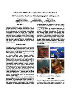
Different representations were evaluated to fit the obtained cloud of samples. A direct representation of the samples distribution can be obtained using a Gaussian, that will form a properly oriented and scaled hyperellipsoid. This is usually simplified as in [10] by using the squared Mahalanobis distance, which may be calculated using computationally expensive algorithms such as Expectation Maximization or second order algorithms such as gradient descent. This representation works well with few samples and it is suitable for online adaptation of a cluster. The problem of this parametric technique is that assumes a known underlying distribution, in this case a normal distribution, which have unimodal densities. Although color classes may present a roughly normal distribution, they usually have convex and concave discontinuities, even holes, due to the codification of color signals. These discontinuities should be noticed for the final cluster, since they might represent regions of possible misclassification. Instead, implicit surfaces were chosen, as they can easily differentiate when samples are inside or outside them, providing a natural interface for color classification. In addition, it is easy to blend different surfaces as in Figure 1. In this way, a set of disjoint samples can produce a continuous surface enclosing all the intermediate points from a color class that are rarely found in sampled images.
Fig. 1. Spherical implicit surfaces for point skeleton primitives, with different blending parameters.
Formally, implicit surfaces, as defined in [11], are two-dimensional, geometric shapes that exist in three dimensional space, defined according to a particular mathematical form. Besides this function, an implicit surface can be easily characterized by its skeleton and a blending function. The skeleton is a set of
primitive elements, such as points and lines, defining individual implicit shapes. The blending function determines the fusion between the individual objects according to their influence. An example of a variation in the blending function is also represented by Figure 1. Our technique can be compared with nonparametric procedures in terms of their capacity for approximating arbitrary clusters with no underlying known distribution. Two well known approaches are the Nearest-neighbor and the Parzenwindow, which can be implemented using a Probabilistic Neural Network, as said in [12]. Although they are powerful methods, they have the drawback of being more complex than the proposed technique, a key point since the desired final application in robotics.
4
Bounding Algorithm
Our approach starts from a set of sample images from which a user selects a set of color samples. A number of primitives is distributed uniformly along the volume of the samples using the k-means algorithm. Once located, the radius of the primitives is obtained from the standard deviation of the samples contained by that primitive. Finally, these primitives are blended to produce the final surface. Figure 2 shows a general overview of this process.
Fig. 2. General description of our approach.
4.1
Distribution of the primitives
To obtain the primitives centers, we use the K-means algorithm. K-means, as defined in [13], is an algorithm for clustering a set of data points into a number of disjoint, non-hierarchical subsets of data points by minimizing a distance criterion. Some options for this criterion are shown in [14]. We selected Euclidean distance, as it describes accurately the color nature in the selected color space; however, it is possible to study different criteria to achieve good results for different applications. K-means is well suited to generate globular clusters, similar to the ones formed by the implicit primitives. Therefore, we conceive the cloud of samples as a big cluster that will be approximated by a group of small clusters defined by N number of primitives. The K-means algorithm will distribute the primitives in the volume occupied by the samples, then adjust iteratively their position to provide each small cluster with a subset of the samples. These samples will be assigned according to the Euclidean distance criterion. The movement is defined by the following process:
1. Calculate the distance from each sample to the primitive center. 2. Move the centroid to the mean of the samples that are closer to the primitive. This process guarantees that every sample will belong to a cluster and that the distribution will converge to a local minimum. Some of the initially declared N clusters will get no samples; they will be eliminated from the final configuration. The initial condition for this process is that each primitive cluster must have at least two samples. For example, if there are ten clusters and only ten samples, five clusters are discarded to guarantee that, if all five are selected as clusters they will have at least the two necessary samples to form a sphere. If, on the contrary we have more than twice samples than the N number of declared primitives, we only use those N primitives to approximate the surface. Another issue is the initial location of the primitives, as a bad initialization will converge to poor results. These locations are determined randomly within the bounding box that contains the cloud of samples using a Gaussian distribution, with more primitives around the centroid of the cloud, where we will probably find more samples, and less in the boundaries.
4.2
Estimation of the radius of the primitives
For each cluster with at least two samples, the standard deviation for the distance to its samples is calculated. The radius of that primitive is set to a multiple S of the standard deviation, according to the next property: For normally distributed data, there is a relation between the fraction of the included data and the deviation from the mean in terms of standard deviations. Part of this relation is shown in Table 1. Table 1. Confidence Interval relation. Fraction of data (%) Number of Standard Deviations from Mean 68.3 1.000 95.4 2.000 99.7 3.000
After calculating the radiuses, we obtain a configuration of primitives that fit the samples cloud. However, we may produce primitives with a large radius but just a few samples. These primitives are said to have low density; meaning that the relation between the primitive size and its samples number is below a threshold U . This could lead to a bigger color class than desired, a problem especially considering possible merge with other classes. To diminish this problem we divide each of those primitives in D new primitives, reapplying the algorithm to the samples in the original primitives.
4.3
Construction of the surface
The reconstruction scheme is based in [15] which creates an implicit surface composed of a set of spherical primitives, defined by: (x − xci )2 + (y − yci )2 + (z − zci )2 (1) ri2 with the following properties: f (P ) < T For all interior points. f (P ) > T For all exterior points. f (P ) = T For all boundary points. where T is a scaling parameter of the sphere, and is set to 1 for simplicity. Primitives are placed in various positions with different radiuses, and then blended with a union function to define the final implicit surface. A differentiable algebraic expression proposed by Ricci [16] is used for this union: fi (P ) =
( q )− n1 X 1 f= For q primitives fn i=0 1
(2)
Here, n is referred as the blending degree; when n approaches to infinity, the function converges to its true minimum. Graphically, this means how tight the surface fits the primitives; a large n means tighter, as illustrated in Figure 3.
Fig. 3. Blending Degree. Left: Small blending degree, Right: Large blending degree.
Through this reconstruction scheme, we will obtain the center and radius of a set of primitives that define an implicit function enclosing the samples. In [15], this reconstruction is obtained by minimizing a cost function, a quadratic sum, representing an error of the desired characteristics in the intended surface. Minimization of this function is neither simple nor fast. Besides, it works directly with samples that lay on the surface and not inside the volume, as the ones used in color classification. A possible solution might be to extract the points that possibly belong to the surface, but many important samples might be lost. One suitable way to perform the data approximation and get the primitives configuration is through a Delaunay Tetrahedronization, as defined in [17], producing a group of tetrahedra that connect all of the sample. Setting a primitive in the center of each tetrahedron and a radius proportional to its volume would yield to a good approximation of the sample data. However, the number of tetrahedra and resulting primitives would be very big, and limiting the number of primitives to the k bigger tetrahedra would result in a poor approximation.
Therefore, we propose a different approach to obtain a configuration of primitives that will approximate a better bounding surface by considering the samples inside of it. While the obtained surface will probably not be the tightest possible to the cloud sample, the color segmentation does not demand a high degree of detail; instead, this provides a higher tolerance for omitted samples.
5
Experimental Results
The algorithm was implemented on a 1.4 MHz Pentium 4 PC with 256 MB memory. The tool works on images or streaming video from an AIBO ERS-210 robot, allowing selecting samples for each color and bound them by an implicit surface. Once the color classes are defined, a look-up table is exported to a text file loaded into a robot for efficient image processing. The configurations produced and the resulting implicit surfaces fit closely the point samples used in the process, producing an accurate representation as depicted in Figure 4.
Fig. 4. Results of configuration of primitives and final implicit surface. Parameters: N=10, D=2,U=2.5, n=2, S=2.
We can also modify iteratively the blending degree. Visually it is interpreted as the “blobbiness” of the bounding surface. Figure 5 exemplifies the effect of this parameter. While a smaller blending degree produces higher robustness in color recognition, a large blending degree can produce accurate results. This is useful to solve collisions between different color classes that are close to each other. A comparison between our approach and a traditional color segmentation technique is shown in Figure 6. In both cases, the same color samples were evaluated to segment the image. It is possible to appreciate that the orange ball is partially recognized as yellow when using cubes; besides, much noise produced by the cube segmentation is automatically filtered in our technique. In Figure 7, a classification is tested in different lighting conditions. The images processed by our algorithm identify colors better even with extreme changes in illumination. This figure also shows the color subspace that is used to identify the color. A traditional approach bounds the samples in this subspace by a cube, leading to misclassifications shown in the lower images. While this tolerance to lighting conditions shows an improvement over traditional techniques, this procedure can be extended to automatically adapt the color subspace dynamically as required by the environment.
Fig. 5. Bounding surface with different blending degrees and the image segmentation for yellow color in a sample image. (a) n=2. (b) n=1.5. (c) n=1.
Fig. 6. Color Classification of a yellow color class. Left: Original image. Center: Image segmentation using our approach. Right: Image segmentation using traditional cubes.
Fig. 7. Robustness to illumination changes. Yellow color is being classified and replaced by blue on the images. Upper row: Image segmentation using our approach with different light intensities. Lower row center: Color subspace used for upper row images. Lower row edges: Image segmentation using traditional cubes on the same images.
Table 2. Time required fitting the surface and reconstructing the look-up table with random initialization for center of primitives. The reconstructed look-up table uses a resolution of 2563 voxels. Number of samples 100-300 300-500 500-700 700-900 900-1100 Time to find primitives (ms) 23 78 197.1 234.4 287.4 Time to create look-up table (ms) 710.9 849.2 968.3 1113.4 1117.6
In addition, the classification process it is notably fast, as seen in Tables 2 and 3. The speed achieved in the approach permits collecting samples interactively in different light conditions, making possible to obtain feedback on the samples almost immediately. Table 3. Time required fitting the surface and reconstructing the look-up table with center initialization based on last adjusted primitives. The reconstructed look-up table uses a resolution of 2563 voxels. Number of samples 100-300 300-500 500-700 700-900 900-1100 Time to find primitives (ms) 17.1 34.1 43.0 44.1 60.0 Time to create look-up table (ms) 766.1 768.1 840.0 887.2 922.5
There are many possible techniques to speed up convergence time and increase precision in the K-means algorithm, as those in [18]. The bottleneck is the conversion of color classes as a look-up table, due to the complexity of evaluating Equation 2 at a high resolution. Although this long evaluation time is permissible for a static offline use, like our classification tool, it is too expensive in a real-time application. Therefore, some other union equations should be evaluated to avoid this issue. Another solution with little impact in the quality of color segmentation is reducing the resolution of the reconstruction space, originally equal to the size of color space (2563 for YUV color signal). Approximations using smaller resolutions considerably reduce the reconstruction time.
6
Conclusions and future work
A new technique for color classification and image segmentation has been proposed. It presents a good approximation of color subspaces even for color signals that are difficult to classify, like YUV, without the need of transforming the current color signal. The surface of the produced subspace bounds tightly the color samples, reducing merging between color classes, and can easily be adjusted to increase tolerance for a given subspace. The algorithm is fast enough to be used interactively and to obtain feedback on the produced segmentation. In the future, we will work with overlapping color classes, in order to derive in some criteria to separate the overlapped subspaces. Moreover, we are developing
an algorithm that permits us to update color samples during the operation of a vision system with the purpose of reaching higher illumination robustness.
Acknowledgments This research is part of “Sensor-Based Robotics” project fully supported by NSF-CONACyT grant under 36001-A and by Tec de Monterrey CEM grant under 2167-CCEM-0302-07. Authors thank Bedrich Benes ITESM-CCM and Neil Hern´andez ITESM-CEM for his comments about this work. This work is part of a MsC Thesis at ITESM-CEM.
References 1. Aceves, A., Junco, M., Ramirez-Uresti, J., Swain-Oropeza, R.: Borregos salvajes 2003. team description. In: RoboCup: 7th Intl. Symp. & Competition. (2003) 2. Junco, M., Ramirez-Uresti, J., Aceves, A., Swain-Oropeza, R.: Tecrams 2004 mexican team. team description. In: RoboCup: 8th Intl. Symp. & Comp. (2004) 3. Bruce, J., Balch, T., Veloso, M.: Fast and cheap color image segmentation for interactive robots. In: Proceedings of WIRE-2000. (2000) 4. Du, Y., Crisman, J.: A color projection for fast generic target tracking. In: IEEE/RSJ Inter. Conf.on Intelligent Robots and Systems. (1995) 5. Oda, K., Ohashi, T., Kato, T., Katsumi, Y., Ishimura, T.: The kyushu united team in the four legged robot league. In: RoboCup: 6th Intl. Symp. & Comp. (2002) 6. Ingo Dahm, Sebastian Deutsch, M.H., Osterhues, A.: Robust color classification for robot soccer. In: RoboCup: 7th Intl. Symp. & Competition. (2003) 7. Nakamura, T., Ogasawara, T.: On-line visual learning method for color image segmentation and object tracking. In: Proc. of IROS’99. (1999) 222–228 8. Wesolkowski, S., Tominaga, S., Dony, R.D.: Shading and highlight invariant color image segmentation. In: Proc. of SPIE. (2001) 229–240 9. Rasmussen, C., Toyama, K., Hager, G.D.: Tracking objects by color alone. DCS RR-1114, Yale University (1996) 10. Ozyildiz, E., Krahnstoever, N., Sharma, R.: Adaptive texture and color segmentation for tracking moving objects. Pattern Recognition 35 (2002) 2013–2029 11. Bloomenthal, J., Wyvill, B.: Introduction to Implicit Surfaces. Morgan Kaufmann Publishers Inc. (1997) 12. Duda, R.O., Hart, P.E., Stork, D.G.: Pattern Classification (2nd Edition). WileyInterscience (2000) 13. Bishop, C.M.: Neural networks for pattern recognition. Oxford Univ. Press (1996) 14. Clustan: k-means analysis. http://www.clustan.com/k-means analysis.html (2004) 15. Lim, C.T., Turkiyyah, G.M., Ganter, M.A., Storti, D.W.: Implicit reconstruction of solids from cloud point sets. In: Proceedings of the third ACM symposium on Solid modeling and applications, ACM Press (1995) 393–402 16. Ricci, A.: A constructive geometry for computer graphics. The Computer Journal 16 (1973) 157–160 17. Zachmann, G., Langetepe, E.: Geometric data structures for computer graphics. In: Proc. of ACM SIGGRAPH. ACM Transactions of Graphics (2003) 18. Elkan, C.: Using the triangle inequality to accelerate k-means. In: Proc. ICML’03. (2003)