and Adaboost) with respect to Ross Quinlan's decision tree inducer C4.5 Release 8 [27] with its default values and its pruning method (all the decision trees ...
Pattern Analysis & Applications (2002)5:201–209 Ownership and Copyright 2002 Springer-Verlag London Limited
Combining Different Methods and Numbers of Weak Decision Trees Patrice Latinne1, Olivier Debeir2 and Christine Decaestecker3 1
IRIDIA (Artificial Intelligence Department), Universite´ Libre de Bruxelles, Brussels, Belgium; 2Information and Decision Systems, Universite´ Libre de Bruxelles, Brussels, Belgium; 3Laboratory of Histopathology, Universite´ Libre de Bruxelles, Brussels, Belgium Abstract: Several ways of manipulating a training set have shown that weakened classifier combination can improve prediction accuracy. In the present paper, we focus on learning set sampling (Breiman’s Bagging) and random feature subset selections (Ho’s Random Subspaces). We present a combination scheme labelled ‘Bagfs’, in which new learning sets are generated on the basis of both bootstrap replicates and random subspaces. The performances of the three methods (Bagging, Random Subspaces and Bagfs) are compared to the standard Adaboost algorithm. All four methods are assessed by means of a decision-tree inducer (C4.5). In addition, we also study whether the number and the way in which they are created has a significant influence on the performance of their combination. To answer these two questions, we undertook the application of the McNemar test of significance and the Kappa degree-of-agreement. The results, obtained on 23 conventional databases, show that on average, Bagfs exhibits the best agreement between prediction and supervision. Keywords: Bagging; Boosting; Decision trees; Ensemble learning; Random subspaces
1. INTRODUCTION Many theoretical and experimental studies have shown that a multiple classifier system is an effective technique for reducing prediction errors [1–6]. From these studies, we identified mainly four groups not mutually exclusive that characterise a Multiple Classifier System (MCS): 쐌 The representation of the input (what each individual classifier receives by way of input). 쐌 The architecture of the individual classifiers (in the learning algorithm and its parameters). 쐌 The architecture of the MCS (parallel, serial or hierarchical, dynamic selection). 쐌 The way in which to combine the classifiers outputs in order to take a decision together. It can be assumed that a combination method is efficient if each individual classifier makes errors ‘in a different way’,
Received: 17 November 2000 Received in revised form: 30 October 2001 Accepted: 13 December 2001
so that it can be expected that most of the classifiers can correct the mistakes that an individual one makes [7]. The term ‘weak classifiers’ [8–11] refers to classifiers whose capacity has been reduced in some way so as to increase their prediction diversity. Either their internal architecture is simple (e.g. they use mono-layer perceptrons or onenearest neighbours), or they are prevented from using all the information available. Since each classifier sees different parts of the learning set, the error correlation among them is reduced [12,13]. It has been shown that the plurality vote is the best strategy if the errors among the classifiers are not correlated. Moreover, in real applications, the plurality vote also appears to be as efficient as more sophisticated decision rules [14–17]. One method of generating a diverse set of classifiers is to upset some aspect of the training input of which the classifier is rather unstable. In the present paper, we study two distinct ways to create such weakened classifiers, i.e. learning set resampling (using the ‘Bagging’ approach [18]), and random feature subset selection (using ‘MFS’, a Multiple Feature Subsets approach [19]). We will compare our results with the boosting method AdaBoost.M1 [20]. Other recent and similar techniques are also based on modifications to the training and/or the feature set [21–23].
202
Bagging is a popular solution for classification problems, and consists of building bootstrap replicates of an original data set and of using these to run a learning algorithm. Quinlan [24] has validated the bagging method with C4.5 decision trees. Once the classifiers have been independently induced from the data (decision tree building), their predictions, made on an independent testing case, are combined with a majority vote rule. Breiman [18] argues that the main reason why bagging works is the instability of the chosen learning algorithm (i.e. decision trees or neural networks) with respect to the variations in the learning set introduced by bootstrapping. The Random Subspace Method consists of training a given number of classifiers (B), with each having as its input a given proportion of features (k) picked randomly from the original set of f features with or without replacement. Ho [25] proposed this approach for decision trees. Bay [19] applied a very similar approach, labeled ‘MFS’, to nearest neighbours. So, like bagging with training patterns, MFS attempts to use classifier instability (this time, with respect to feature selection) to generate a set of classifiers with uncorrelated errors (see also Zheng [23] and Breiman [26]). In the rest of the paper, we will called this second type of weakening method ‘MFS’. The standard boosting algorithm, Adaboost.M1 [20,24], generates a set of classifiers sequentially (the next classifier depends upon the classification results of the previous one performed on the learning set), while bagging generates them independently. Adaboost changes the weights of the training examples by increasing the weights of the misclassified examples. The goal is to force the learning algorithm to minimise the expected error over different input distributions: the classifiers are combined by a weighted voting rule, the weight of each classifier depending upon its performance on the learning set used to build it.
2. MATERIAL AND METHODS To take qualitative advantages of both techniques (bagging and MFS), we investigated their combination in the same architecture we labelled ‘Bagfs’. For this purpose, we generated B bootstrap replicates of the learning set (those used to apply the bagging). In each replicate we independently sampled a subset of f⬘ features, randomly selected from amongst the f initial ones without replacement. We denoted k = f⬘/f as the proportion of features in these B subsets (the same subsets of features were used to apply ‘MFS’). The proposed architecture thus has two parameters, B and k, to be set. We combined the B predictions made on an independent test set with respect to the plurality voting rule. We tested the different algorithms (bagging, MFS, Bagfs and Adaboost) with respect to Ross Quinlan’s decision tree inducer C4.5 Release 8 [27] with its default values and its pruning method (all the decision trees were pruned). C4.5 was adapted to handle the instance weights used by Adaboost, as specified by Quinlan [24]. We applied bagging, MFS, Bagfs and Adaboost to 23 databases (see Table 1). Of these, 18 were downloaded from
P. Latinne et al.
Table 1. Databases used to assess the classification tasks Data set
Training set size
Testing set size
# Feat.
# Class
glass irisa ionosphere liver disorders new-thyroid breast-cancer-wb wine car diabetes hepatitisb,c soybeanb,c annealingb,c
214 150 351 345 215 699 178 1728 768 155 307 798
– – – – – – – – – – 376 100
9 4 34 6 5 9 13 6 8 19 35 38
6 3 2 2 3 2 3 4 2 2 19 5
ringnorma twonorma satimage waveforma waveform 40a image phoneme texturea gauss 8D abalonec lettera
7400 7400 6435 5000 5000 2310 5404 5500 5000 3133 4000
– – – – – – – – – 1044 16000
20 20 36 21 40 18 5 40 8 8 16
2 2 6 3 3 7 2 11 2 28 26
a
Databases where the examples are equi-distributed across the classes Databases that have missing values c Databases that have nominal features b
the UCI Machine Learning Repository [28], i.e. iris, wine, glass, ionosphere, BUPA liver disorders, image segmentation, new thyroid gland, waveform (with or without 20 noisy features), Wisconsin breast-cancer, car evaluation, soybean, annealing, hepatitis, Pima Indian diabetes, abalone, satimage, letter. We also included Ringnorm and Twonorm, two artificial databases used by Breiman [29]. Finally, we downloaded other classical problems from the ELENA’s project repository (ftp.dice.ucl.ac.be/pub/neural-nets/ELENA/databases) : gauss 8D, texture and phoneme. Several databases are reported as being divided into a learning and a testing set (soybean, annealing, abalone, letter). For these databases, the experimental design will be the same, except that no global crossvalidation is required.
3. EXPERIMENTAL DESIGN In the present paper, we investigate the benefit of using different ways to weaken a learning set to create diverse decision-trees: learning set bootstrapping and multiple feature selections. This is illustrated by the three methods described above, namely bagging, MFS and Bagfs. We also compared these methods to the boosting method, Adaboost.M1.
Combining Methods and Numbers of Weak Decision Trees
203
The comparisons were made with the same number of classifiers (B = 200), and we studied the impact of increasing the number of classifiers from 1 to 200. For the databases that have no separated testing set, a stratified 10-fold crossvalidation was performed. Evaluations and comparisons were made on the basis of the same learning and testing set resulting from each stratified 10-fold cross-validation. For all the smallest databases (fewer than 200 examples), 10 replications of the experiment were also performed to validate our estimates. The degree-of-agreement coefficient () was computed between the test pattern predictions and the corresponding true classes (supervision). was proposed by Rosenfield et al [30]. It represents an efficient accuracy measurement that estimates the level of agreement (1) after any chance agreement (2) has been discarded (see also Siegel et al [31] and Rosner [32]):
=
1 − 2 1 − 2
(1)
= 1 if the prediction agrees perfectly with the supervision, = 0 if this agreement is obtained by chance, and ⬍ 0 if it is worse than that obtained by chance. In this paper, we use the McNemar test [31–33] as a direct method for testing whether two sets of predictions differ significantly among themselves. Given the two algorithms A and B, this test compares the number of examples misclassified by A, but not by B (labelled Mab), with the number of examples misclassified by B, but not by A (labelled Mba). In the case that Mab ⫹ Mba ⱖ 20, if the null hypothesis H0 is true (i.e. if there is no difference between the algorithms’ predictions), then the statistics X2 can be considered as following an 2 distribution (with 1 degree of freedom): X2 =
(兩Mab − Mba兩 − 1)2 苲 21 Mab + Mba
(2)
H0 is rejected if X2 is greater than 21 = 3.841459 (significance level p ⬍ 0.05). In this case, the algorithms have significantly different levels of performance. As for the evaluation, we applied this test to the complete set of predictions performed during every cross-validation on each database. If condition Mab ⫹ Mba ⱖ 20 is not satisfied, the approximation of the statistical distribution cannot be used and the exact test described in Rosner [32] has to be performed. As it happened rarely in our experimental design, in these cases, we preferred to accept the hypothesis that the two algorithms have the same performance. Moreover, different studies (see, for instance, [33,34] showed that this non-parametric test is also preferred to parametric ones (such as the commonly used t-test), because no assumption is required and it is independent of any evaluation measurement (error rate, degree of agreement kappa, etc.). Dietterich [34] has also shown that McNemar has a low type I error (the probability of incorrectly detecting a difference when no difference exists), and concluded that it is one of the most acceptable tests among the most common ones if the algorithms can only be executed once.
4. RESULTS AND DISCUSSION Table 2 shows the results of the estimated accuracy based on the degree-of-agreement, . The last two columns represent the proportions of selected features (kopt) and the corresponding number of features. kopt is the effective proportion of features obtained by maximising when performing a stratified 10-fold cross-validation on each learning set. We used this nested cross-validation process to keep one testing set independent of the data used for the training and tuning of the internal parameter, k. This nested cross-validation was applied to Bagfs and MFS, and for each database we identified the same kopt value for these two algorithms (i.e. the kopt value reported in Table 2). Table 2 also shows the usefulness of this nested crossvalidation process to determine kopt values. Indeed, when kopt is larger than 0.5 (in the case of seven different databases), MFS systematically exhibited lower results than bagging and Bagfs. Bagfs also suffered from this since it was never better than bagging in these situations. This indicates that the MFS contribution of Bagfs is not useful when a large proportion of features is required. So, if the nested cross-validation reveals that kopt ⬎ 0.5, then we may conclude that MFS is not an appropriate way of weakening a classifier, and should not be used. In Table 3, we also computed the standard error rate ⫾ standard deviation to be directly comparable to other similar studies (see, for instance, [21,24]). The results in Tables 2 and 3 show that Bagfs was a competitive method when used on these 23 databases, even against Adaboost. On each database, Bagfs had always at least the same level of performance than the best method among bagging and MFS. Adaboost outperformed Bagfs on ‘car evaluation’ data base only. Tables 4 and 5 reports the results of a strict comparison of the four algorithms (bagging, MFS, Bagfs and Adaboost) with respect to McNemar test statistics performed on the 23 databases. This comparison is strict in the sense that, for the small databases (i.e. N ⬍ 2000), as we performed 10 replications of the experiments, we concluded that the compared algorithms differed significantly if the McNemar H0 hypothesis is rejected on six replications or more with a p ⬍ 0.05 level of significance. For the large databases, we performed only one test on the total set of predictions. In Table 4, a bold value designates a data base for which the compared models differ significantly with respect to McNemar. Tables 4 and 5 report that Bagfs performed significantly better with respect to McNemar test than bagging or MFS on at least eight databases and than Adaboost on four databases (Adaboost is significantly better than Bagfs on ‘car evaluation’). Bagfs outperformed significantly both bagging and MFS on four databases. Why Bagfs works better can be explained by observing the influence on the global accuracy estimates of the induced diversity and error decorrelation between all the combined classifiers. Dietterich [21] recently used the index as a measurement of the ‘diversity’ between two classifier predictions.
204
P. Latinne et al.
Table 2. Prediction accuracy in terms of degree-of-agreement estimates Data set
C4.5
Bag200
MFS200
Bagfs200
Boost200
kopt
(f⬘/f)
glass iris iono bupa new-thyroid breast-cancer-w wine car diabetes hepatitis soybean annealing
0.563 0.920 0.792 0.220 0.861 0.884 0.880 0.839 0.438 0.319 0.689 0.280
0.650 0.910 0.820 0.422 0.895 0.916 0.924 0.850 0.460 0.400 0.722 0.335
0.660 0.915 0.856 0.225 0.830 0.938 0.984 0.839 0.433 0.396 0.869 0.298
0.686 0.915 0.856 0.437 0.881 0.936 0.982 0.851 0.449 0.425 0.878 0.332
0.677 0.916 0.828 0.434 0.898 0.933 0.940 0.947 0.466 0.409 0.774 0.320
0.4 0.5 0.4 0.7 0.3 0.2 0.3 0.8 0.7 0.4 0.6 0.8
(4/9) (2/4) (13/33) (5/6) (2/5) (2/9) (4/13) (5/6) (6/8) (8/20) (21/35) (32/38)
ringnorm twonorm satimage waveform waveformn image phoneme texture gauss8D abalone letter
0.829 0.693 0.837 0.644 0.623 0.966 0.688 0.916 0.706 0.117 0.869
0.912 0.936 0.891 0.757 0.758 0.973 0.751 0.967 0.777 0.157 0.931
0.955 0.939 0.900 0.765 0.767 0.972 0.699 0.978 0.754 0.134 0.952
0.964 0.948 0.898 0.779 0.780 0.972 0.742 0.976 0.784 0.157 0.950
0.944 0.944 0.898 0.779 0.780 0.974 0.750 0.976 0.784 0.159 0.877
0.4 0.5 0.5 0.5 0.5 0.4 0.7 0.3 0.5 0.8 0.4
(8/20) (10/20) (18/36) (11/21) (20/40) (13/33) (4/5) (12/40) (4/8) (7/8) (7/16)
Mean
0.677
0.741
0.739
0.762
0.757
Table 3. Prediction accuracy in terms of the global error rate estimates ⫾ standard deviation Data set
C4.5
Bag200
MFS200
Bagfs200
Boost200
glass iris iono bupa new-thyroid breast-cancer-w wine car diabetes hepatitis soybean annealing
0.321 0.053 0.094 0.374 0.065 0.053 0.079 0.074 0.251 0.200 0.287 0.310
0.257 ⫾ 0.024 0.060 ⫾ 0.000 0.080 ⫾ 0.006 0.275 ⫾ 0.023 0.048 ⫾ 0.010 0.038 ⫾ 0.006 0.050 ⫾ 0.004 0.069 ⫾ 0.004 0.238 ⫾ 0.014 0.173 ⫾ 0.019 0.257 ⫾ 0.008 0.267 ⫾ 0.007
0.244 ⫾ 0.037 0.057 ⫾ 0.017 0.065 ⫾ 0.006 0.362 ⫾ 0.034 0.073 ⫾ 0.009 0.028 ⫾ 0.004 0.011 ⫾ 0.002 0.074 ⫾ 0.000 0.247 ⫾ 0.009 0.156 ⫾ 0.015 0.119 ⫾ 0.004 0.282 ⫾ 0.010
0.226 ⫾ 0.033 0.057 ⫾ 0.009 0.065 ⫾ 0.006 0.266 ⫾ 0.026 0.052 ⫾ 0.012 0.029 ⫾ 0.005 0.012 ⫾ 0.002 0.069 ⫾ 0.004 0.239 ⫾ 0.013 0.154 ⫾ 0.028 0.111 ⫾ 0.003 0.246 ⫾ 0.010
0.235 ⫾ 0.032 0.056 ⫾ 0.011 0.075 ⫾ 0.019 0.268 ⫾ 0.029 0.046 ⫾ 0.009 0.031 ⫾ 0.006 0.039 ⫾ 0.014 0.024 ⫾ 0.004 0.234 ⫾ 0.018 0.179 ⫾ 0.039 0.207 ⫾ 0.005 0.252 ⫾ 0.010
ringnorm twonorm satimage waveform waveformn image phoneme texture gauss8D abalone letter
0.085 0.154 0.132 0.237 0.251 0.029 0.131 0.076 0.147 0.786 0.127
0.044 ⫾ 0.006 0.032 ⫾ 0.006 0.088 ⫾ 0.010 0.162 ⫾ 0.012 0.161 ⫾ 0.022 0.023 ⫾ 0.011 0.103 ⫾ 0.017 0.030 ⫾ 0.008 0.112 ⫾ 0.014 0.746 ⫾ 0.006 0.126 ⫾ 0.001
0.022 ⫾ 0.004 0.030 ⫾ 0.007 0.081 ⫾ 0.008 0.156 ⫾ 0.011 0.155 ⫾ 0.020 0.024 ⫾ 0.011 0.125 ⫾ 0.011 0.020 ⫾ 0.007 0.123 ⫾ 0.017 0.775 ⫾ 0.004 0.094 ⫾ 0.001
0.018 ⫾ 0.005 0.026 ⫾ 0.007 0.082 ⫾ 0.007 0.147 ⫾ 0.012 0.151 ⫾ 0.019 0.024 ⫾ 0.011 0.107 ⫾ 0.016 0.022 ⫾ 0.007 0.108 ⫾ 0.019 0.745 ⫾ 0.005 0.093 ⫾ 0.001
0.028 ⫾ 0.005 0.028 ⫾ 0.007 0.086 ⫾ 0.008 0.148 ⫾ 0.010 0.147 ⫾ 0.024 0.022 ⫾ 0.009 0.103 ⫾ 0.019 0.218 ⫾ 0.007 0.108 ⫾ 0.016 0.742 ⫾ 0.009 0.118 ⫾ 0.001
Mean
0.188
0.150 ⴞ 0.010
0.145 ⴞ 0.011
0.132 ⴞ 0.011
0.148 ⴞ 0.013
Combining Methods and Numbers of Weak Decision Trees
205
Table 4. McNemar test resultsa Data set
Bag MFS
McN
Bagfs MFS
McN
Bag Bagfs
McN
Boost Bagfs
McN
glass iris iono bupa new-thyroid breast wine car diabetes hepatitis soybean annealing
138 12 33 522 93 35 0 187 417 34 56 34
166 17 86 223 41 107 70 102 353 60 575 19
0 0 0 10 0 3 10 0 0 0 10 0
97 9 14 530 46 9 0 188 391 38 62 36
58 9 14 198 2 16 2 101 334 34 31 0
0 0 0 10 3 0 0 0 0 0 0 0
82 5 26 63 51 46 0 1 198 14 44 11
149 10 79 96 43 111 68 3 191 44 594 32
0 0 0 0 0 2 9 0 0 2 10 0
82 11 36 98 51 53 5 856 226 44 53 34
107 10 72 107 37 62 55 82 181 84 415 51
0 0 1 0 0 0 3 10 1 1 10 0
ringnorm twonorm satimage waveform waveformn image phoneme texture gauss8D abalone letter
57 52 58 169 147 19 231 29 196 117 74
216 66 104 198 176 16 114 85 138 89 146
1 0 1 0 0 0 1 1 1 0 1
49 64 46 133 138 9 204 13 177 141 58
17 32 55 86 95 8 106 24 101 97 82
1 1 0 1 1 0 1 0 1 1 0
36 43 64 127 100 17 86 32 124 64 100
227 89 101 203 172 15 67 77 142 80 148
1 1 1 1 1 0 0 1 0 0 1
32 51 52 124 129 16 78 36 120 58 341
107 68 77 130 128 12 57 36 120 56 763
1 0 1 0 0 0 0 0 0 0 1
a
We indicated for each comparison two columns containing the Mab and Mba values for the total number of trials (10 for small databases and one for large ones). In each McN column, a value indicates the number of replications of the experimental design for which the hypothesis that the models are identical is rejected with respect to McNemar
Table 5. Summary of the McNemar test resultsa McNemar
Bag200
MFS200
Bagfs200
Bag200 MFS200 Bagfs200
– 6–3 9–0
3–6 – 8–0
0–9 0–8 –
a On 23 databases, numbers of times the algorithm indicated in the row has significant better-worse levels of performance than the algorithm in the column
In this case, the index was computed on a confusion table crossing the predictions made by the two classifiers. We used a similar approach here, and thus disposed of the index as both diversity and accuracy of the base classifiers. The results, obtained on the 23 databases, all lead to the same overall observations. Figure 1 illustrates four representatives diagrams for which the algorithms compared are significantly different with respect to the McNemar test. Each dot in Fig. 1 corresponds to a pair of classifiers included in the different combination schemes. Each possible pair is characterised by the kappa index computed on both the agreement between the predictions of the two classifiers
(1 ⫺ is reported on the x coordinate as a measurement of the diversity of these classifiers) and that between prediction and supervision averaged over the two classifiers (reported on the y coordinate as a measurement of the accuracy of these classifiers). These figures show that individual Bagfs classifiers always exhibit a greater degree of diversity than bagging and MFS, and also a lower level of accuracy (each individual classifier is weaker, on average). So, to obtain an effective weak multiple classifier system, we expect to have a scatter plot where the dots are in the high diversity and low individual accuracy regions. Moreover, all these results were obtained with 200classifier systems. One important question may be to know if it is necessary to build so many trees to obtain similar results. This is crucial in many applications with large databases like the classification of millions of pixels in remote-sensing, for instance, for which multiple classifier systems are efficient but rather time-consuming. When creating multiple classifier systems such as bagging, MFS and Bagfs, we would like to avoid overproducing an arbitrary large number, B, of voting classifiers. We propose here to apply the McNemar test again to measure the impact of the number of base classifiers on prediction accuracy. We applied the McNemar test of significance as described in Section 3 between two sets of predictions from two MCSs
206
P. Latinne et al.
Fig. 1. Diversity – accuracy diagrams in terms of the Kappa degree-of-agreement.
that differ only in their number of classifiers. Let us denote L as a learning set and T = {(x, y)} as a data set independent from L. Let Cm = {yˆ = vote{(k) (x, L), k = 1, . . . , m}} be the prediction set of m voting classifiers. The classifiers (k) are built so that the classifier predictions are diverse and on an equal footing in terms of voting (non-weighted plurality vote): no classifier is a priori better than another with respect to any criterion (i.e. this is not the case for boosting-like algorithms). The proposed procedure consists of comparing the prediction set Cm to Cn, with n ⬎ m, with respect to the McNemar test. Either the set of classifiers used to obtain predictions Cn is entirely independent from that which predicts Cm, or it contains all or part of the m classifiers that predicts Cm. Our results showed that this does not change the conclusion of the experiment. The McNemar test gives an answer d(m, n) with respect to a significance level (here, p ⬍ 0.05):
冦
1
if H0 rejected and Mmn ⬎ Mnm
d(m, n) = −1 if H0 rejected and Mnm ⬎ Mmn 0
if the two prediction sets do not differ
If d(m, n) = 1, then McNemar concludes that combining n classifiers gives a higher level of performance than combining m classifiers with respect to the McNemar test. If d(m, n) = ⫺1, it may only appear rarely, since increasing the number of voting classifiers should not degrade the prediction accuracy significantly. In fact, this case never appeared in our experiments.
If d(m, n) = 0, then combining m weakened classifiers does not significantly differ from combining n. For five large databases and the different methods (bagging, MFS and Bagfs), we performed a stratified threefold cross-validation. One fold is used for building 200 decision trees with respect to each weakening method and the remaining part to apply the McNemar test. In Fig. 2, for each method and database, each dot represents the mean of each table d(m, n), obtained from the three-fold crossvalidation (i.e. the result of the McNemar test that compares the prediction set of an m-classifier system (on a row) with the prediction of an n-classifier system (on a column) (m, n = 1..200)). Each diagram is composed of a bright and a dark region (d(m, n) took only the values ⫺1 and 0; d(m,n)=⫺1 never appeared in our experimental framework). The dark region means that the compared architectures differ significantly with respect to McNemar (p ⬍ 0.05). The bright region means that the architectures compared do not differ significantly. These results show that a threshold appeared distinctly between the two regions ‘differ’ or ‘differ not significantly’. We are able to find a minimum number of trees required to obtain a prediction accuracy not significantly different from those obtained by combining larger numbers of trees. On ‘satimage’, Bagfs needed approximately at least 50 trees, while MFS and bagging required (respectively) at least 60 and 20 trees. On ‘letter’, Bagfs required 90 trees, bagging required 90 trees and MFS required at least 50 trees. Therefore, we conclude that the McNemar test is a strict significance measure of combining many trees to obtain a better
Combining Methods and Numbers of Weak Decision Trees
207
Fig. 2. Influence of the number of trees on the predictions with respect to the McNemar test.
prediction accuracy. The McNemar test might be useful to find a ‘minimum’ but secure number of trees to combine, obtained on a validation set, and then to use this number of trees on a larger number of new data to be scored. Any post-processing method could thereafter be applied to select a subset of ‘good’ trees to combine with respect to an optimal criterion (see, for instance, Giacento and Rol: [35]).
5. CONCLUSION This paper compares four methods for generating multiple learning sets: bagging, random subspaces, Adaboost and a novel approach, labelled ‘Bagfs’, that mixes bagging and random subspaces. These methods were applied with the C4.5 algorithm. For each method, 200 trees were built. By
208
a strict application of a statistical method (the McNemar test), we investigated the significant differences between these methods of weakening decision trees in terms of classification accuracy. The experimental results obtained on 23 conventional databases showed that Bagfs differed significantly from bagging and random subspaces on at least eight databases and on five databases in comparison with Adaboost. We showed that Bagfs never performed worse, and performed even better than the other models combining the same number of classifiers (except that Adaboost outperformed Bagfs on one database). We illustrated on several representative databases, for which the models were significantly different with respect to the McNemar test, that Bagfs’ base classifiers had a higher level of diversity and a lower level of accuracy than the classifiers in the other models. If the optimal proportion of selected features (determined a priori by a nested cross-validation) is too large (⬎ 50% of the total number of features), we showed that random subspaces was not an appropriate method to increase prediction accuracy (and Bagfs had the same level of performance than bagging). Furthermore, we investigated the use of the McNemar test to measure the impact of the number of base classifiers, on prediction accuracy. We showed that a limited number of base classifiers, once combined with the plurality voting rule, offered the same level of performance than larger numbers, with respect to the McNemar test. First results showed on five real databases that the three methods, bagging, random subspaces and Bagfs, required smaller numbers of trees to be as accurate as the combination of larger numbers of trees. Acknowledgements
Patrice Latinne and Olivier Debeir are supported by a grant under an ARC (Action de Recherche Concerte´ e) programme of the Communaute´ Franc¸ aise de Belgique. Christine Decaestecker is a Research Associate with the ‘F.N.R.S’ (Belgian National Scientific Research Fund).
References 1. Ho TK. Data complexity analysis for classifier combination. Proceedings 2nd International Workshop of Multiple Classifier System, Cambridge, UK. Lecture Notes in Computer Science, Springer-Verlag, 2001; 2096:53–67 2. Ho TK, Hull JJ, Srihari SN. Decision combination in multiple classifier systems. IEEE Trans Pattern Analysis and Machine Intelligence 1994; 16(1):66–75 3. Huang YS, Suen CY. A method of combining multiple experts for the recognition of unconstrained handwritten numerals. IEEE Trans Pattern Analysis and Machine Intelligence 1995; 17(1) 4. Kittler J. Combining classifiers: a theoretical framework. IEEE Trans Pattern Analysis and Applications 1998; 1:18–27 5. Lam L. Classifier combinations: implementations and theoretical issues. Proceedings 1st International Workshop of Multiple Classifier System, Cagliari, Italy. Lecture Notes in Computer Science, Springer-Verlag, 2000; 1857:77–86 6. Xu L, Krzyzak A, Suen CY. Methods of combining multiple classifiers and their applications to handwriting recogntion. IEEE Trans Systems, Man and Cybernetics 1992; 22(3):418–435
P. Latinne et al. 7. Ali KM, Pazzani MJ. Error reduction through learning multiple descriptions. Machine Learning 1996; 24:173–202 8. Dietterich TG, Kearns M, Mansour Y. Applying the weak learning framework to understand and improve c4.5. Proceedings 13th International Conference on Machine Learning. Morgan Kaufmann Publishers, 1996; 96–104 9. Ji and Ma. Combinations of weak classifiers. IEEE Trans Neural Network 1997; 7(1):32–42 10. Jiang W. Some theoretical aspects of boosting in the presence of noisy data. Proceedings 18th International Conference on Machine Learning, Williams, MA, 2001; 234–241 11. Schapire RE. The strength of weak learnability. Machine Learning 1990; 5:197–227 12. Oza NC, Tumer K. Input decimation ensembles: Decorrelating through dimensionality. Proceedings 2nd International Workshop of Multiple Classifier System, Cambridge, UK. Lecture Notes in Computer Science, Springer-Verlag, 2001; 2096:238–247 13. Tumer K, Ghosh J. Classifier combining: analytical results and implications. Proceedings National Conference on Artificial Intelligence – Workshop in Induction of Multiple Learning Models, Portland, OR, 1996 14. Battiti R, Colla AM. Democracy in neural nets: voting schemes for classification. Neural Networks 1995; 7(4):691–708 15. Duin RPW, Tax DMJ. Experiments with classifier combining rules. Proceedings 1st International Workshop of Multiple Classifier System, Cagliari, Italy. Lecture Notes in Computer Science, Springer-Verlag, 2000; 1857:16–29 16. Lam L, Suen CY. Application of majority voting to pattern recognition: an analysis of its behavior and performance. IEEE Trans Systems, Man and Cybernetics 1997; 27(5) 17. Perrone M. Putting it all together: methods for combining neural networks. Advances in Neural Information Processing Systems 6, 1994; 1188–1189 18. Breiman L. Bagging predictors. Machine Learning 1996; 24 19. Bay SD. Nearest neighbor classification from multiple feature subsets. Proceedings 15th International Conference on Machine Learning, Madison, WI, 1998 20. Freund and Schapire. A decision-theoretic generalization of online learning and an application to boosting. J Computer and System Sciences 1997; 55(1):119–139 21. Dietterich TG. An experimental comparison of three methods for constructing ensembles of decision trees: bagging, boosting and randomization. Machine Learning 2000; 40:139–157 22. Kohavi R, Kunz C. Option decision trees with majority votes. Proceedings 14th International Conference on Machine Learning, San Francisco, CA, 1997; 161–169 23. Zheng Z. Generating classifier committees by stochastically selecting both attributes and training examples. Proceedings 5th Pacific Rim International Conferences on Artificial Intelligence (PRI-CAI’98), Springer-Verlag, 1998; 12–23 24. Quinlan JR. Bagging, boosting, and c4.5. Proceedings 13th National Conference on Artificial Intelligence 1996; 725–730 25. Ho, TK. The random subspace method for constructing decision forests. IEEE Trans Pattern Analysis and Machine Intelligence 1998; 20:832–844 26. Breiman L. Random forests – random features. Technical Report 567, Statistics Department, University of California, Berkeley, CA 94720, September 1999 27. Quinlan JR. C4.5: Programs For Machine Learning. Morgan Kaufmann, San Mateo, CA 1993 28. Blake C, Keogh E, Merz CJ. Uci respository of machine learning databases. [http://www.ics.uci.edu/mlearn/MLRepository.html]. University of California, Department of Information and Computer Science, 1998 29. Breiman L. Arching classifiers. Annals of statistics 1998; 26:801–849
Combining Methods and Numbers of Weak Decision Trees 30. Rosenfield GH, Fitzpatrick-Lins K. A coefficient of agreement as a measure of thematic classification accuracy. Photogrammetric Engineering and Remote Sensing 1986; 52(2):223–227 31. Siegel S, Castellan NJ. Nonparametric Statistics for the Behavioral Sciences. McGraw-Hill, 2nd ed, 1988 32. Rosner B. Fundamentals of Biostatistics. Duxbury Press (ITP), Belmont, CA, 4th ed, 1995 33. Salzberg S. On comparing classifiers: Pitfalls to avoid and a recommended approach. Data Mining and Knowledge Discovery 1997; 1:317–327 34. Dietterich TG. Approximate statistical tests for comparing supervised classification learning algorithms. Neural Computation 1998; 10:1895–1923 35. Giacento G, Roli F. Dynamic classifier selection based on multiple classifier behaviour. Pattern Recognition Letters 2001; 34(9):179–181
Patrice Latinne received his MS from the Universite´ Libre de Bruxelles (ULB) in mechanical and electrical engineering in 1998 and his ‘Diplome d’Etudes Approfondies’ in applied sciences in 2001. He is currently achieving his PhD in the Institute of Interdisciplinary Research and Development in Artificial Intelligence (IRIDIA, ULB). He is supported by a grant under an ARC (Action de Recherche Concerte´ e) programme of the Communaute´ Franc¸ aise de Belgique. His research interests are data analysis, machine learning, pattern recognition applied among others to medical diagnosis, remote sensing and quality control.
209
Olivier Debeir received his MS from the Universite´ Libre de Bruxelles (ULB) in mechanical and electrical engineering in 1995 and his ‘Diplome d’Etudes Approfondies’ in applied sciences in 2001. He is currently working on his PhD in the Information and Decision Systems Department (ULB). He is supported by a grant under an ARC (Action de Recherche Concerte´ e) programme of the Communaute´ Franc¸ aise de Belgique. His research interests are artificial intelligence, decision tree algorithms, computer vision applied, among others, to medical diagnosis aid to melanoma detection and remote sensing.
Christine Decaestecker obtained her MS in mathematics in 1984 from the Universite´ Libre de Bruxelles (ULB), where she also received her PhD in pure science in 1991. From 1992 to 1996 she was at the Institute of Interdisciplinary Research and Development in Artificial Intelligence (IRIDIA, ULB) for research projects involving data analysis, pattern recognition, machine learning and neural networks. Since 1994, she has collaborated with the Laboratory of Histopathology (Faculty of Medicine, ULB), which she joined in 1996, to develop computerassisted methods aiming to establish new prognostic and diagnostic markers in the cancer field. This research was the subject of her ‘Agre´ gation de l’Enseignement Supe´ rieur’ thesis (qualification for university professorship). Since October 1999 she has been a Research Associate with the Belgian FNRS at the Laboratory of Histopathology (ULB).
Correspondence and offprint requests to: P. Latinne, IRIDIA (Artificial Intelligence Department), Universite´ Libre de Bruxelles, CP 194106, 50 Franklin Roosevelt, Brussels B-1050, Belgium. E-mail:platinne얀ulb.ac.be