Combining Formal Verification and Testing for ... - Semantic Scholar

Combining Formal Verification and Testing for Correct Legacy Component Integration in Mechatronic UML! Holger Giese1 , Stefan Henkler2 , and Martin Hirsch2 1

Hasso Plattner Institute for Software Systems Engineering at the University of Potsdam, Prof.-Dr.-Helmert-Str. 2-3, D-14482 Potsdam , Germany 2 Software Engineering Group, University of Paderborn, Warburger Str. 100, D-33098 Paderborn, Germany [email protected], {shenkler-mahirsch}@uni-paderborn.de Abstract. One of the main benefits of component-based architectures is their support for reuse. The port and interface definitions of architectural components facilitate the construction of complex functionality by composition of existing components. For such a composition means for a sufficient verification either by testing or formal verification are necessary. However, the overwhelming complexity of the interaction of distributed real-time components usually excludes that testing alone can provide the required coverage when integrating a legacy component. In this paper we present a scheme on how embedded legacy components can be tackled. For the embedded legacy components initially a behavioral model is derived from the interface description of the architectural model. This is in the subsequent steps enriched by an incremental synthesis using formal verification techniques for the systematic generation of component tests. The proposed scheme results in an effective combination of testing and formal verification. While verification is employed to tackle the inherently subtle interaction of the distributed real-time components which could not be covered by testing, local testing of the components guided by the verification results is employed to derive refined behavioral models. The approach further has two outstanding benefits. It can pin-point real failures without false negatives right from the beginning. It can also prove the correctness of the integration without learning the whole legacy component (using the restrictions of the integration context).

1 Introduction The main benefits of the component-based architectures are their support for information hiding and reuse. The interface of a component is well defined by structural elements and collaboration protocols (cf. [7]). The dependencies between components are reduced to the knowledge of the known interfaces or ports. Thereby, a component can be exchanged if the specified port remains fulfilled. The port and interface definitions of !

This work was developed in the course of the Special Research Initiative 614 - Self-optimizing Concepts and Structures in Mechanical Engineering - University of Paderborn, and was published on its behalf and funded by the Deutsche Forschungsgemeinschaft.

R. de Lemos et al. (Eds.): Architecting Dependable Systems V, LNCS 5135, pp. 248–272, 2008. c Springer-Verlag Berlin Heidelberg 2008 !

Combining Formal Verification and Testing

249

architectural components therefore facilitate the construction of complex functionality by composition of existing components. Especially in domains like automotive software where the development of new functions is an exception rather than the regular case (cf. [48]) component-based development can result in dramatic improvements. However, as long as an open and flexible software architecture which facilitate reuse is missing, many functions are nearly built from scratch for each new version (cf. [25]). Today, initiatives such as AUTOSAR1 are a first step towards open and flexible software architectures for automotive systems. The definition of standard interfaces and an infrastructure for the software components ensures that components from different suppliers and vendors can technically interoperate. However, also a correct integration at the application level is needed. In general, the proper composition of independently developed components in the software architecture of embedded real-time systems requires means for a sufficient verification of the integration step either by testing or formal verification. However, the overwhelming complexity of the interaction of distributed real-time components usually excludes that testing alone can provide the required coverage when integrating a legacy component. Today, often a model-based development approach is employed to plan the decomposition of complex systems into components which are developed by different suppliers. The M ECHATRONIC UML approach is one approach which permits to plan the decomposition of complex real-time systems upfront. It supports the description and compositional verification of the real-time coordination by means of components and patterns [24] and the integrated description and modular verification of discrete behavior and continuous control with components [9,21]. While it also supports for the generation of code for hard real-time processing [8,10] from further refined models in practice, seldom the whole system will be generated from the models. Besides the automatically derived components also either manually programmed or already existing components which fit more or less to the M ECHATRONIC UML models will be employed. Thus an approach is required which permits to integrate these legacy components not only syntactically but also provide the required verification guarantees. The overwhelming complexity of the interaction of distributed real-time components usually excludes that testing alone can provide the required coverage when integrating a legacy component. Thus formal verification techniques seem to be a valuable alternative. However, the required verification of the resulting system often becomes intractable as no abstract model of the reused components which can serve the verification purpose is available. A number of techniques which either use a black-box approach and automata learning [32] or a white-box approach which extracts the models from the code [39,15,31] exists. However none of them exploits the knowledge about the context and a component-based view to provide an approach which could in principle scale even for larger systems and which can help excluding besides false positives also false negatives after a feasible number of learning steps. In this paper we present a scheme how embedded legacy components in a M ECHA TRONIC UML architecture can be tackled based on our approach presented in [29]. For the embedded legacy components initially a behavioral model is derived from the 1

www.autosar.org

250

H. Giese, S. Henkler, and M. Hirsch

existing interface description which is a safe abstraction. This abstraction is then in subsequent steps enriched by an incremental synthesis procedure. This procedure uses the counterexample of a formal verification step to improve the accuracy of the behavioral model of the legacy component. We extend our previous work by supporting a (safe) over approximation and a rigorous formalization of the approach. The formal verification step based on [21,24] is employed to cover the inherently subtle interaction of the distributed real-time components completely which could not be achieved by testing. Local testing of the legacy components using our model-based testing approach [23] and our approach for deterministic replay [22] guided by the verification results in the form of counterexamples is employed to derive refined behavioral models for the legacy component. The approach therefore extends our former work [21,22,23,24,29] and has the benefit that it could pin-point real failures in the test step which are no false negatives right from the beginning. In addition, it can also prove the correctness of the integration for an abstract behavioral model of the legacy component without learning the whole legacy component by only checking possible integration problems for the explicit given context. Application Example As a concrete example for a complex mechatronic product, we use a simplified version of the software for the RailCab research project2 . The vision of the RailCab project is a mechatronic rail system where autonomous shuttles apply the linear drive technology, used in the Transrapid, but travel on the existing passive track system of the standard railway. One particular problem, which has been previously described in [24], is to reduce the energy consumption due to air resistance by coordinating the autonomously operating shuttles in such a way that they form convoys whenever possible. Such convoys are created on-demand and require small distances between the shuttles in order to achieve significant energy savings. Coordination between the speed control units of the shuttles becomes a safety-critical aspect and results in a number of hard real-time constraints, which have to be addressed when building the control software of the shuttles. In [24] it has been solved for a simplified version of this shuttle coordination problem. In this example convoys consist of at most 2 shuttles. The main requirement of the shuttle controller software is to ensure that no rearend collision happens when the first shuttle has to brake suddenly e.g., in case of an emergency. If the shuttle is the head of a convoy it may brake only with reduced force, because another shuttle drives behind it with a reduced, minimal distance and therefore reacts with delay. Therefore the controlling software needs to ensure that the following situation will never occur: The rear shuttle is in convoy mode and therefore reduces the distance and the front shuttle is in mode no-convoy and brake with full strength in case of an emergency. Modeling Within our modeling and verification approach for the software of complex real-time systems [24], modeling is divided into modeling the interaction between components of the system by reusable coordination patterns and modeling the detailed behavior of the components by relating to the behavior of the applied patterns. 2

http://www-nbp.upb.de/en/index.html


251

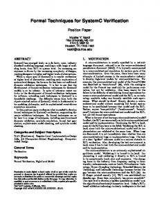
A pattern describes communication and therefore consists of multiple communication partners, called roles. Roles interact through ports which are linked by a connector. The communication behavior of a role is specified by a real-time statechart (RTSC) and is restricted by an invariant. The behavior of the connector is described by another real-time statechart that is used to model channel delay and reliability, which are of crucial importance for real-time systems. The overall behavior of a pattern is restricted by a pattern constraint, whereas the behavior of a role can be restricted by a role invariant. Altogether, we call the constraints, invariants, and known communication partners context information Within the shuttle example, distance coordination between two shuttles is modeled as a pattern. This DistanceCoordination pattern consists of two roles, the frontRole and the rearRole and one connector that models the wireless radio link between the two shuttles. The pattern specifies the behavior needed to coordinate two successive shuttles. The main requirement of the pattern is to ensure that no rear-end collision happens when the first shuttle has to brake suddenly, e.g. in case of an emergency. If the shuttle is the head of a convoy, it is allowed to brake only with reduced force, to ensure that it cannot collide with the shuttle which drives behind it with a reduced, minimal distance. Otherwise, as the follower shuttle will react with a certain delay, a collision might happen. We thus require that the front shuttle must not brake with full power if it is in convoy mode. For the rear shuttle, we require that it does brake with full power. These two requirements are called role invariants. On the other hand, the overall pattern constraint forbids the rear role to be in mode convoy while frontRole is in mode noConvoy. The pattern constraint and role invariants can be annotated to the pattern respectively its roles using timed ACTL3 formulas. The pattern with its annotated constraint and invariants is depicted in Figure 1. true A[] not deadlock A[] not (rearRole.convoy and frontRole.noConvoy)

unsafe A[] not deadlock DistanceCoordination A[] not (myRearRole.convoy and myFrontRole.convoy) frontRole rearRole

Shuttle2

Shuttle3

Fig. 1. The DistanceCoordination pattern

After the patterns have been specified, the concrete software components can be built. Components are designed by coordinating and refining each role RTSC of the involved patterns. The refinement has to respect the role RTSC (i.e. not add additional behavior or block guaranteed behavior) and additionally has to respect the guaranteed behavior of the roles in the form of their invariants. An additional internal RTSC for coordination is used to describe the required coordination of the refined roles. We further refer to the refined roles as component ports or ports in short. 3

Timed ACTL is the subset of timed computation tree logic [13] which only contains always path operators.

252


In our example, the shuttle component must conform to the DistanceCoordination pattern and has to operate as both a rearRole and a frontRole as it may be follow, or be followed by, another shuttle as well as itself can follow another shuttle. To complete the presented approach the outlined modeling capabilities are further extended by model checking and code generation. We prove that the given constraints hold for the system by using a model checker. Code generation on the other hand ensures that the constraints still hold for the code. However, in practice frequently not the whole system will be generated from the models. Instead several independent developed or already existing components that have been not automatically derived from M ECHATRONIC UML models have to be integrated (cf. Figure 2). Approach Given a M ECHATRONIC UML architecture which embeds a legacy component and behavioral models for all other components building the context of the legacy component, the basic question of correct legacy component integration is whether for the composition of the legacy component and its context all anomalies such as deadlocks are excluded or all additionally required properties hold. However, it is usually very expensive and risky to reverse-engineer an abstract model of the legacy component to verify whether the integration will work. To overcome this problem we suggest employing some learning strategy via testing to derive a series of more detailed abstract models for the legacy component. The specific feature of our approach will be that we exploit the present abstract model of the context to only test relevant parts of the legacy component behavior. The approach depends only to a minimal extent on reverse engineering results. We start with synthesizing a model of the legacy component behavior based on known structural interface description and a reverse engineered upper bound on the state size. Then, we check whether the context plus the model of legacy behavior exhibit any undesired behavior taking generic correctness criteria or additional required properties into account. If not, we use the resulting counterexample trace to test the legacy component. If the trace can be realized with the legacy component, a real error has been found. If not, we first enrich the trace with additional information using deterministic replay and then merge the enriched trace into the model of the legacy component behavior. We repeat the checks until either a real error has been found or all relevant cases have been covered. Figure 2 illustrates our process with a summary of the overall approach. 1) Initially, we synthesize an initial behavior model for the legacy component based on known structural interface description and derive a behavioral model of the context from the existing M ECHATRONIC UML models. 2) We check the combination of the two behavioral models and either get a) a counterexample or b) the checked properties are guaranteed. In the latter case we are done. 3) If we have a counterexample, we use this as test input for the legacy component. Deterministic replay enables us to enrich the observable behavior with state information by monitoring. If the tested faulty run is confirmed, we have found a real counterexample. If not, we can use the new observed behavior to refine the previously employed behavior model of the legacy component. We repeat steps 2) to 4) until one of the described exits occurs.


253

1

Extract behavioral model of context

Synthesize behavior

Mcontext

Mlegacy

4

Observed behavior Counterxample (Input vector)

3

Execute legacy component

[Counterexample confirmed]

2

Check combination

Mlegacy Mcontext

[Properties satisfied]

Produce output

Fig. 2. Sketch of the approach

Overview We first define in the next Section the prerequisite of our approach. We will introduce incomplete automata and chaotic automata which are required for learning the behavior. In Section 3 we describe the initial behavior synthesis and in Section 4 we describe the iterative process for behavioral synthesis. Based on the counterexamples from Section 4, we describe in Section 5 our testing approach. Section 6 compares our work to similar approaches and Section 7 presents the conclusion and future work.

2 Prerequisites To provide a formal ground for our later employed M ECHATRONIC UML concepts, we present a formal definition for the employed notion of automata, parallel composition, and refinement as well as the employed compositionality results for this formal model. The RTSC employed in M ECHATRONIC UML are mapped to a finite state transition system in the form of extended Kripke structures (called I/O-interval structures [44]). We present here only a rather simplified version of this finite state transition model where discrete time is mapped to single states and transitions. This automata model is sufficient to permit the understanding of the underlying behavior model and to prove that the compositional verification combined with the testing and monitoring is correct. The simplification is justified by the following assumption which are valid for the considered domain: (1) the usual clock synchronization assumption which is common to many systems and means that time is progressing equally fast in any system component, and (2) a discrete time model suffices to model all time depending constraints, because the underlying infrastructure (hardware and possibly a real-time operating systems) does not react infinitely fast. The simplified real-time automaton model and its real-time processing which corresponds to our employed notion of RTSC are defined as follows: Definition 1. An automaton is a 5-tuple M = (S, I, O, T, Q) with a finite set S of states, input signals I, output signals O, a set of transitions T ⊆ S × ℘(I) × ℘(O) × S where ℘(X) denotes the power-set of X, and the initial state set Q. The behavior is characterized by execution sequences called runs.

254


Definition 2. A regular run is a sequence of states and I/O π = s1 , A1 /B1 , s2 , . . . , where for each i ≥ 1 exists (si , Ai , Bi , si+1 ) ∈ T . We in addition have deadlock runs which are a sequence of states and I/O π = s1 , A1 /B1 , s2 , . . . sn , An /Bn , where for each 1 ≤ i ≤ n exists (si , Ai , Bi , si+1 ) ∈ T and & ∃sn+1 (sn , An , Bn , sn+1 ) ∈ T . We write [M ] for the set of all regular and deadlock runs and use π|I/O to restrict a run to an observable trace and π|S to denote the related state sequence.4 The time semantics of an automaton is simply that each transition takes exactly one time unit. For convenience we use in the following Si , Ii , Oi , Ti , and Qi to denote the corresponding elements of Mi . Two automata M and M ! with distinct input and output sets (I ∩ I ! = ∅ and O ∩ O! = ∅) are further called composable. If also I ∩ O! = ∅ and O ∩ I ! = ∅ holds, they are even orthogonal to each other. 2.1 Property Specification Properties which should hold for a specific model are specified by using clocked CTL (CCTL) constraints (φ) and invariants (ψ). These formulas will be build using a shared set of atomic propositions P . An automaton Mi and any of its states s ∈ Si is annotated with all propositions in Pi ⊆ P which they fulfill using a labeling function Li : S → ℘(Pi ). Thus an automaton Mi = (Si , Ii , Oi , Ti , Qi ) is accordingly extended to a 6tuple Mi = (Si , Ii , Oi , Ti , Li , Qi ). The label set L(Mi ) denotes the set of all by the labeling considered propositions Pi . L(φ) and L(ψ) denote the subsets of the basic proposition set P that is employed within the formulas. Finally, for sake of simplification of the following formal definitions, we omit any syntactical details of CTL and CCTL and write M |= φ when an automaton M fulfills a constraint or invariant φ. The special symbol δ is used to denote that a deadlock (a state without any outgoing transition) can be reached. M |= ¬δ thus denotes that M does not contain any deadlocks. 2.2 Parallel Composition In our application domain the composition of multiple components requires their parallel execution. As we model time explicitly and in a discrete manner, the required notion of parallel composition must result in the synchronous execution [13] of all systems running in parallel. The communication is formalized by synchronous communication such that sending and receiving happens within the same time step. Consequently, the asynchronous event semantics of statecharts is modeled by explicitly defined event queues (channels) given in the form of additional automata. These explicit models of the event queues are required anyway to take the QoS characteristics of each connection into account. To combine two composed automata we simply connect their input and output signals and consider their parallel execution. 4

The concepts outlined here have some similarities with process algebra concepts. While regular runs reduced to the observable events are traces in CSP [30] or other process algebras, deadlock runs are related to ideas of failures in CSP or refusals. In contrast to the presented proposal, process algebra approaches abstract from states.


255

Definition 3. For two automata M = (S, I, O, T, L, Q) and M ! = ! ! ! ! ! ! (S , I , O , T , L , Q ) which are composable to each other (I ∩ I ! = ∅ and O ∩ O! = ∅), we define their parallel composition denoted by M +M ! as the automaton (S !! , I !! , O!! , T !! , L!! , Q!! ) with S !! = S × S ! , I !! = I ∪ I ! , O!! = O ∪ O! , Q!! = Q × Q! , and ((s1 , s!1 ), A!! , B !! , (s2 , s!2 )) ∈ T !! iff (s1 , A, B, s2 ) ∈ T and (s!1 , A! , B ! , s!2 ) ∈ T ! exist with A!! = A ∪ A! and B !! = B ∪ B ! . Additionally, (A ∩ O! ) = B ! and (A! ∩ O) = B must hold. S !! and T !! are further adjusted to exclude all non reachable state combinations and transitions. The labelling L!! for (s, s! ) ∈ S !! is easily derived as L!! ((s, s! )) = L(s) ∪ L! (s! ).

Informally, a transition in T !! is a combination of two transitions in each automaton iff all required local inputs by the other side are matching ((A ∩ O! ) = B ! and (A! ∩ O) = B) and the non local input and output signals are simply the union of both automata. 2.3 Automata Refinement

Our restricted notion of components means that they are derived by refining the role protocols from all the patterns they are participating in. Thus, we require an appropriate notion for refinement which is essentially a restricted version of simulation which additionally preserves reactivity. For two given automata we can define whether the first is a refinement of the second as follows. Definition 4. An automaton M = (S, I, O, T, L, Q) is a refinement of automaton M ! = (S ! , I ! , O! , T ! , L! , Q! ) (M - M ! ) iff hold: ∀π = . . . s ∈ [M ]∃π ! = . . . s! ∈ [M ! ] : π|I/O = π ! |I ! /O! ∧ L(s) = L! (s! )

(1)

∀π = . . . s, A/B ∈ [M ]∃π = . . . s! , A/B ∈ [M ! ] : π|I/O = π ! |I ! /O!

(2)

For each path in the refinement M equation 1 further ensures that a related path in M ! exists. Equation 2 further ensures that every deadlock path of M is also a possible deadlock path for M ! . Therefore, - implies simulation (0). 2.4 Compositional Constraints For our approach the interesting class of constraints is the constraints, which are preserved under refinement and composition with disjoint labeling. Definition 5. A constraint φ is compositional iff for any automaton M1 , M1! , and M2 with L(M2 ) ∩ L(φ) = ∅ holds (M1 |= φ) ⇒ ((M1 +M2 |= φ) ∨ (M1 +M2 |= δ)) and ((M1 - M1! ) ∧ (M1! |= φ)) ⇒ (M1 |= φ)

(3) (4)

CTL formulas are preserved by the bisimulation equivalence relation, while ACTL formulas are preserved by the simulation preorder (0) [13]. The presented refinement implies simulation and thus preserves ACTL formulas also, but in contrast it additionally preserves deadlock freedom:

256


Lemma 1. For automaton M and M ! with M - M ! holds M ! |= ¬δ ⇒ M |= ¬δ. Proof. (sketch) Condition 1 ensures that for any s ∈ S at least one related s! ∈ S ! exists with (s, s! ) ∈ Ω. From M ! deadlock free follows that s! will have at least one outgoing transition and due to condition 2 s also. Therefore, M is also deadlock free. Invariants, upper and lower time-bounds, and ACTL formulas in general are constraints which refer only to all possible paths. Thus using the fact that a refinement or composition with disjoint labeling sets only reduces the possible sequences of states with identical labeling, they are compositional. That deadlock freedom is also compositional follows by construction for condition 3 and Lemma 1 for condition 4. Compositionality can thus be established for the properties required so far during our studies such as deadlock freedom, upper bounds for the maximal delays of message transports, lower bounds for the minimal delays of message transports, and invariants. For example, the according CCTL formula with only A path quantifiers for a maximal delay is for d the maximal delay, p1 the trigger condition, and p2 the required condition: AG(¬p1 ∨ (AF [1,d] p2 )). In contrast, temporal logic formulas that demand explicitly that a specific state is eventually reached (abstracting from possible effects of nondeterminism) are not preserved. 2.5 Parallel Composition and Refinement We also require that parallel composition preserves refinement. Lemma 2. For any automaton M1 and an automaton M2 refining automaton M2! (M2 - M2! ) holds M2 - M2! ⇒ (M1 +M2 - M1 +M2! ). Proof. (sketch) For M1 +M2! we can form the construction of the parallel composition conclude that only path and deadlock path result which are also present in M1 +M2 . Therefore condition 1 and 2 must be fulfilled for M1 +M2 and M1 +M2! . For a substitution of a restricted refinement that only adds disjoint I/O signals we further have to prove that compositional constraints and deadlock freedom are preserved. Lemma 3. For automaton M1 , M2 , and M2! with M2 -I/O M2! , I1 ∩ (O2 − O2! ) = ∅, O1 ∩ (I2 − I2! ) = ∅, and L(M1 ) ∩ (L(M2 ) − L(M2! )) = ∅ and any compositional constraint φ holds (M1 +M2! |= φ ∧ ¬δ) ⇒ (M1 +M2 |= φ ∧ ¬δ)

(5)

Proof. Due to φ and ¬δ being compositional and Definition 5 we can for M2!! = M2 |I2! /O2! /L(M2! ) conclude that M1 +M2!! |= φ ∧ ¬δ or M1 +M2!! |= δ. Due to Lemma 1 and 2 we even have M1 +M2!! |= φ∧¬δ. From I1 ∩(O2 −O2! ) = ∅ and O1 ∩(I2 −I2! ) = ∅ follows that M2 adds to M2!! only I/O that does not interfere with M1 and thus M1 +M2 has the same reachable state set and transitions and thus M1 +M2 |= ¬δ. As φ is only interpreted over states and the labeling is identical for L(φ) ⊆ L(M2! ), φ must also hold and thus condition 5 is proven.


257

2.6 Incomplete Automata When incrementally improving the accuracy of a behavioral model with respect to some original, we can use the concept of a incomplete automaton. Definition 6. An incomplete automaton is a 6-tuple M = (S, I, O, T, T , Q) with M = (S, I, O, T, Q) an automaton and T ⊆ S × ℘(I) × ℘(O) denoting the known not supported interactions. To ensure that T and T are consistent we require that ¬(∃s, A, B, s! : (s, A, B, s! ) ∈ T ∧ (s, A, B) ∈ T ). The behavior is characterized by execution sequences called runs. Definition 7. A regular run of an incomplete automaton is a sequence of states and I/O π = s1 , A1 /B1 , s2 , . . . , where for each i ≥ 1 exists (si , Ai , Bi , si+1 ) ∈ T . We in addition have deadlock runs which are a sequence of states and I/O π = s1 , A1 /B1 , s2 , . . . sn , An /Bn , where for each 1 ≤ i ≤ n exists (si , Ai , Bi , si+1 ) ∈ T and (sn , An , Bn ) ∈ T . We write [M ] for the set of all regular and deadlock runs and use π|I/O to restrict a run to an observable trace and π|S to denote the related state sequence. The definition of the runs highlights the fact that in an incomplete automaton deadlock runs are only assumed when explicitly defined by T and not implicitly if no transition is present in T . A concrete automaton is deterministic if for any s, A, and B holds that |{(s, A, B, s! ) ∈ T }| ≤ 1. An incomplete automaton is deterministic if for any s, A, and B holds that |{(s, A, B, s! ) ∈ T } ∪ {(s, A, B) ∈ T }| ≤ 1. Given an incomplete automaton, we can then describe a completion step as any extension of S, T or T which again results in an incomplete automaton. In a final step an incomplete automata becomes complete, when for each possible interaction is either forbidden by T or present in T : ∀s ∈ S, A ∈ ℘(I), B ∈ ℘(O) : (∃s! ∈ S : (s, A, B, s! ) ∈ T xor (s, A, B) ∈ T ). 2.7 Chaotic Automata and Closure Taking the refinement notion of Definition 4, we can identify a maximal behavior (named chaotic automaton) which is an abstraction of every possible behavior as it might accept any sequence of inputs but may also deadlock for every possible interaction. Definition 8. For given input and output sets I and O, the chaotic automaton Mc = (Sc , I, O, Tc , Qc ) is build as follows: The state set Sc = {sδ , s∀ } contains two distinct state, the transition set Tc = {(s∀ , A, B, s∀ )|A ∈ ℘(I), B ∈ ℘(O)} ∪ {(s∀ , A, B, sδ )|A ∈ ℘(I), B ∈ ℘(O)}, and Qc = {sδ , s∀ }.

The chaotic automaton specified in Definition 8 is depicted in Figure 35 . We can see that both state s∀ and sδ are possible initial states and that while sδ will block any 5

Note, we write in all figures and listings s all and s delta and not s∀ and sδ as the mathematical notation is not supported by the used tool.

258


s_all *

*

s_delta

Fig. 3. Maximal chaotic behavior: the chaotic automaton

interaction, s∀ will support any possible interaction (all possible input and output combinations are referred to here by ’*’). If also a number of properties are relevant, we have to further have states s∀ and sδ for every possible proposition subset P ! of P . However, it is much more efficient to instead label s∀ and sδ with a new proposition p! and replace for all propositions p ∈ P all occurrences of p by (p ∨ p! ) as well as occurrences of ¬p by (¬p ∨ p! ). If we are interested in a safe abstraction, a special kind of completion is the chaotic completion where all defined behavior result in arbitrary chaotic behavior. Definition 9. Given an incomplete automaton M = (S, I, O, T, T , Q) we derive the related chaotic closure automaton M ! = (S ! , I, O, T ! , Q! ) as follows: 1. double the state set and include the chaotic automaton (S ! = (S × {0}) 4 (S × {1}) 4 Sc ) and 2. adjust the transition set to the doubling such that all not specified interactions either are not supported or lead to the added chaotic automaton (T ! = {((s, 0), A, B, (s! , 0)|(s, A, B, s! ) ∈ T } 4 {((s, 0), A, B, (s! , 1)|(s, A, B, s! ) ∈ T } 4 {((s, 1), A, B, (s! , 0)|(s, A, B, s! ) ∈ T } 4 {((s, 1), A, B, (s! , 1)|(s, A, B, s! ) ∈ T } 4 {((s, 1), A, B, s∀ )|s ∈ S, a ∈ ℘(I), B ∈ ℘(O), (s, A, B) &∈ T } 4 {((s, 1), A, B, sδ )|s ∈ S, a ∈ ℘(I), B ∈ ℘(O), (s, A, B) &∈ T } 4 Tc .

We denote the chaotic closure of M as chaos(M ).

In this construction Q! = {(s, 0)|s ∈ Q} 4 {(s, 1) ∈ Q}. The states (s, 0) are those representing the case that no further extension is assumed which might thus result in a deadlock, while the states (s, 1) are those representing the case that all possible further extensions are assumed which therefore lead to chaos (which is represent by sδ and s∀ ). Note that this chaotic behavior is highly non-deterministic while the real legacy component behavior is required to be deterministic. 2.8 Observation Conformance and Refinement Definition 10. The incomplete automaton M is observation conforming concerning an automaton Mr iff [M ] ⊆ [Mr ]. Note that the defined notion of observation includes states in our case, while in a standard setting we would only consider the path. Theorem 1. If M is an observation conforming incomplete automaton concerning a concrete deterministic component implementation Mr , it holds that Mr - chaos(M ).


259

Proof. Condition 1 for refinement follows directly from [M ] ⊆ [Mr ] as we let sδ and s∀ fulfil all positive and negative propositions (by modifying the formulas accordingly). Condition 2 is fulfilled as the chaotic closure guarantees by construction only additional behavior which can always also result in a deadlock. !

3 Initial Behavior Synthesis Given a concrete context Mrc with abstract model Mac that refines the concrete context (Mrc - Mac ) and a concrete component implementation Mr with hidden internal details (legacy component), the basic question we want to check is whether a given property φ as well as deadlock freedom (¬δ) holds. We are in particular interested in a guarantee that both properties hold or a counterexample witnessing that they do not hold. However, usually Mr cannot be employed to traverse the whole state space as the state space of the system Mac +Mr is too large to directly address this question. To overcome this problem we suggest to build a series Mai of abstractions of Mr which are all safe when it comes to verification but become more and more accurate such that finally we can use them to conclude either that the integration works correctly or not. (6) Mr - Mai (∀i ≥ 0).

We thus start with synthesizing a model of the legacy component behavior based on the known structural interface description. While the interface description can be taken from the context or reverse-engineered straightforwardly from the legacy component, deriving an upper bound on the relevant legacy component states can become more complicated. The crucial criterion for a valid state abstraction is that for all possible inputs/outputs the state reached must be the same. In a first step we simply build Ma0 using the available information about the interface of Mr . We simply build an Ml0 by determining the initial state s0 of Mr and derive an automaton Ml0 = ({s0 , I, I, ∅, {so}). We can then use the chaotic closure to derive our first safe approximation: Ma0 = chaos(Ml0 ). Due to Theorem 1 we then know that Ma0 is a safe abstraction from Mr (Mr - Ma0 ). Lemma 4. For the initial model Ma0 = chaos(Ml0 ) for Ml0 build for the initial state s0 of Mr as the automaton Ml0 = ({s0 , I, I, ∅, {so }) holds Mr - Ma0 .

Proof. Due to Theorem 1 we can conclude that Ma0 is a safe abstraction from Mr as Ml0 is observation conforming to Mr . !

In Figure 4(a) the initial trival automaton is depicted. The automaton consists of an initial state (depicted as a double circle) and the first state noConvoy::default which is connected via a transition with the initial state. The automaton which results when the chaotic closure is applied to the trivial incomplete automaton depicted in Figure 4(a) which only captures the known initial state noConvoy::default is depicted in Figure 4(b). We can see how this initial state has been doubled and that one of these two states is connected via any possible interaction with both chaotic states s∀ and sδ (all possible input and output combinations are referred to here by ’*’).

260


noConvoy::default

*

s_all

*

*

noConvoy::default

(a)

s_delta

noConvoy:default

(b)

Fig. 4. Trivial initial implicit automaton encoding the known initial state (4(a)) and Initial behavior of a legacy component (4(b)) convoyProposal? noConvoy::default

breakConvoy! convoy::break

convoyProposalRejected!

breakConvoyProposal?

noConvoy::answer

startConvoy! convoy::default

breakConvoyRejected!

Fig. 5. Known behavior of context

In Figure 5 the known behavior of the context, the frontrole, is depicted. The automaton starts in the noConvoy state. The automaton remains in the state until the frontRole receives the convoyProposal message. Thereafter the automaton switches to the answer state. In this state, the automaton non-deterministically decides to reject the convoy (convoyProposalRejected) or to start the convoy (startConvoy). In the latter case the automaton switches to the convoy state and remains there until a breakConvoyProposal message is received. The automaton decides to reject or accept this message.

4 Iterative Behavior Synthesis On the basis of the initial behavior synthesis, we describe in this section our approach of iterative behavior synthesis. First, we start with checking if the given properties hold for the initial synthesized behavior. If a counterexample exists, we proceed with testing based on that counterexample. While testing we monitor the legacy system. The monitored trace is used for learning the behavior. The new synthesized behavior is then the start point for the next iteration. 4.1 Formal Verification Step The iterative behavior synthesis starts with checking for the abstraction derived from initial behavior synthesis (cf. Section 3), whether a counterexample for the required property φ exists. We therefore check for i ≥ 0 Mac +Mai |= φ ∧ ¬δ.

(7)

If the check succeeded, we have indeed proven that the property must also hold for Mac +Mr and Mrc +Mr .


261

Lemma 5. Given a concrete context Mrc with abstract model Mac and a concrete component implementation Mr with derived abstraction Mai such that the concrete context refines the abstract context (Mrc - Mac ) and that the abstraction is valid (Mr - Mai ) it holds for any compositional property φ: Mac +Mai |= φ

⇒

Mrc +Mr |= φ.

(8)

Proof. As refinement (-) is a precongruence for parallel composition (+) and Mrc Mac , we can conclude that Mrc +Mai - Mac +Mai must hold. Similarly, having Mr - Mai we thus have Mrc +Mr - Mac +Mai . As refinement preserves property φ, we thus can starting with Mac +Mai |= φ conclude that Mrc +Mr |= φ must hold. ! If, however, the check did no succeed, we will have a counterexample in the form of a path π for Mac +Mai which is a witness that φ is not true for the abstraction. This counterexample restricted to Mai is then used to test the legacy component. Listing 1.1. Initial counterexample shuttle1.noConvoy, shuttle2.s_all, shuttle2.convoyProposal!, shuttle1.convoyProposal? shuttle1.answer, shuttle2.wait, shuttle1.convoyProposalRejected!, shuttle2.convoyProposalRejected? shuttle1.noConvoy, shuttle2.s_all shuttle2.convoyProposal!, shuttle1.convoyProposal? shuttle1.answer, shuttle2.wait shuttle1.startConvoy!, shuttle2.startConvoy? shuttle1.convoy, shuttle2.s_all shuttle2.breakConvoyProposal!, shuttle1.breakConvoyProposal? shuttle1.break, shuttle2.s_delta

In Listing 1.1 the counterexample of the first check is shown. The counterexample is a relatively long run. First, the closure sends a convoyProposal to the context. Afterwards, the context sends a convoyProposalReject. Then, the closure sends once again a convoyProposal and the context decides to build a convoy by sending a startConvoy. After building the convoy, the context tries to break the convoy but the closure goes in sδ state and a deadlock is manifested. 4.2 Testing Step If the test reveals that the path π is also possible in the concrete system, we can conclude that we have found a real integration problem. Lemma 6. Given a concrete context Mrc with abstract model Mac and a concrete component implementation Mr with derived abstraction Mai such that the concrete context refines the abstract context (Mrc - Mac ) and that the abstraction is valid (Mr - Ma0 ) it holds: ! c " Ma +Mai , π &|= φ ∧ π ∈ Mrc +Mr ⇒ Mrc +Mr &|= φ (9)

Proof. As π is a witness of ¬φ and φ is a run of Mrc +Mr we can conclude that Mrc +Mr &|= φ must hold. !

262


If we use our trick to weaken the properties rather than using a chaotic closure which distinguishes all possible subsets of the atomic properties P , it seems that we have to evaluate φ on Mrc +Mr , π to check that the counterexample is a real one. As this could only happen when π visits states in the chaotic closure (s∀ or sδ ) it is guaranteed that in these cases π is not really a possible run of Mrc +Mr as the concrete state will never include states of the chaotic closure. It is to be noted we assume that for runs the encoding (s, i) with i ∈ {0, 1} is considered equivalent to s and therefore runs which are only visiting these states can be mapped to runs in the legacy component and therefore result in uncover real counterexamples. If the run cannot be found when testing the legacy component, we can use the observed difference between π and the really observed behavior π ! to derive an improved Mai+1 . In our example, if we test the legacy component based on the counterexample shown in the last Section with the techniques described in Section 5, we monitor the trace shown in Listing 1.2. As described in the next Section when testing the legacy component, we only monitor relevant events for deterministic replay. Hence, we monitor only the outgoing message convoyProposal at port rearRole and the incoming message convoyProposalRejected at the same port. If we look in more detail at the behavior while deterministically replay the legacy component with all relevant instrumentation for monitoring additionally the states and timing, the trace shows a conflict with expected behavior based on the initial counterexample (cf. Listing 1.3). In the next Section, we will shown, how conflict is manifested while checking the synthesized behavior based on the monitored traces. Listing 1.2. Monitored relevant events for deterministic replay: blocking state [Message] name="convoyProposal", portName="rearRole", type="outgoing" [Message] name="convoyProposalRejected", portName="rearRole", type=incoming

Listing 1.3. Monitoring all relevant events: blocking state [CurrentState] name="noConvoy" [Message] name="convoyProposal", portName="rearRole", type="outgoing" [Timing] count=1 [CurrentState] name="convoy", [Message] name="convoyProposalRejected", portName="rearRole", type=incoming

4.3 Learning Step In this learning step we employ the observed difference between π and the really observed behavior π ! to derive an improved Mli+1 . Then we derive Mai+1 again as chaos(Mli+1 ) and have due to Theorem 1 by construction: Mr - Mai+1 ,

(10)

as π ! is an observable behavior of Mr and all other behavior still present in Mli+1 is already present in Mli .


263

For learning we have to distinguish two cases. First, a previously unobserved behavior π ! has been recorded. We can then do the learning as follows: Definition 11. Given a deterministic incomplete automaton M = (S, I, O, T, T , Q) and a regular run π, we derive the deterministic incomplete automaton M ! = (S ! , I, O, T ! , T , Q! ) which results from learning π (denoted by learn(M, π)) as follows: S ! = S ∪ {s &∈ S|π = . . . s . . . }, T ! = T ∪ {(s, A, B, s! ) &∈ T |π = . . . s(A, B)s! . . . }, and Q! = Q ∪ {s &∈ Q|π = s . . . }.

A second case is present, when the test was blocked. In this case we have a deadlock run π of the form . . . s(A, B) where (A, B) has been blocked in state s. Learning will then work as follows. Definition 12. Given a deterministic incomplete automaton M = (S, I, O, T, T , Q) and a deadlock run π = . . . s(A, B) where the last interaction was blocked, we derive ! the deterministic incomplete automaton M ! = (S, I, O, T, T , Q) which results from ! learning π (denoted by learn(M, π)) as follows: T = T ∪ {(s, A, B)}.

In both cases a learned behavior results in a safe abstraction, as shown in the following lemmata. Lemma 7. Given a concrete context Mrc with abstract model Mac and a concrete component implementation Mr with derived abstraction Mai such that the concrete context refines the abstract context (Mrc - Mac ) and that the behavior learned so far is valid (Ma0 is observation conforming to Mr ) holds for any possible run π of Mrc +Mr : Mr - Mai+1 for Mai+1 = chaos(learn(Mli , π)).

(11)

Proof. It follows form the construction that learn(Mli , π) is like Mli observation conforming to Mr . Due to Theorem 1 refinement for chaos(learn(Mli , π ! )) follows. ! In order to be able to employ a trace to improve our abstraction, we only require that the implementation Mr is deterministic while Mai might include non-determinism. This is, however, no real limitation, as in the domain of safety-critical systems we will build components such that any non-determinism or pseudo non-determinism is excluded. In our example, we have synthesized the automaton shown in Figure 6. First, the legacy component is in a noConvoy state. When sending the covnoyProposal message, the legacy component switches in state convoy. 4.4 Multiple Iterations With the outlined procedure we can systematically derive a series of abstraction Ma0 , Ma1 , . . . , Man such that we stepwise improve our knowledge about the legacy component Mr . In contrast to other approaches for learning this series guarantees always refinement such that we can stop our efforts if a first n has been found with Mac +Man |= φ noConvoy

convoyProposal! convoy

Fig. 6. Synthesized behavior: conflict with environment

264


as this implies that φ also holds for the real system (Mrc +Mr |= φ). If in contrast we reach an n where the related counterexample πn can also be detected in the real implementation Mrc +Mr and thus the counterexample is also one for the implementation. Theorem 2. Given a concrete context Mrc with abstract model Mac such that the concrete context refines the concrete context (Mrc - Mac ) and a concrete component implementation Mr with derived series of abstractions {Mai |0 ≤ i ≤ n} constructed as outlined in Lemma 7, we can decide whether a property φ holds for Mrc +Mr or continue the series. Proof. (sketch) We can show that Mli is observation conforming to Mr ∀0 ≤ i ≤ n via induction. The first step of the induction is: Lemma 4 provides the guarantee that we will always at least have one first element Ml0 in the series. Thus we can assume the condition for n = 0. In the induction step we show that if the series can be continued for i, Lemma 7 guarantees the condition also holds for i + 1. If we cannot continue the series, we either have proven φ for Mac +Man or the counterexample πn is also present for Mrc +Mr . In the former case du to Lemma 5 we have proven the property φ for Mrc +Mr . In the latter, Lemma 6 allows us to conclude that the property φ is also violated by Mrc +Mr . Thus, we can either continue the series or prove respectively disprove the property φ. ! For finite state legacy components, we can even guarantee termination of this process. Assuming a finite number of states and transitions as well as deterministic behavior of the legacy component, every time where the counterexample could not be observed during testing, we will replace chaotic behavior by previously unknown states or transitions. Therefore, the number of not already captured states and transitions is strict monotonically decreasing with each iteration round. As it cannot fall below zero, the iterative process will thus terminate. Based on the synthesized behavior shown in Figure 6, we build a closure and check it with the context. Listing 1.4 shows the counterexample. The property A[] not (rearRole.Convoy and frontRole.noConvoy) is violated. The trace shows, that the violation is only in the synthesized part of the model and therefore, we have a proof that the legacy component is in conflict with context! This example shows, that our approach supports a fast conflict detection. Listing 1.4. Counterexample with conflict in synthesized behavior shuttle1.noConvoy, shuttle2.noConvoy shuttle2.convoyProposal!), shuttle1.convoyProposal? shuttle1.answer, shuttle2.convoy

The approach supports besides possible fast conflict detection a systematic/automatic way of testing all relevant input combination of the context with respect to the specification (properties). The input for testing is the same as shown in the conflicting example


265

(cf. Listing 1.1). The monitoring trace shows, that all interactions are performed by the legacy component with respect to the test input. The synthesized behavior, shown in Figure 7 confirm this observation. When checking the synthesized behavior containing the closure, a deadlock is manifested in the closure and not only in the synthesized part of the behavior. Hence, we will get a counterexample, which we can use as test input for the next step. Listing 1.5. Succesful learning step: monitoring all relevant events [CurrentState] name="noConvoy::default" [Message] name="convoyProposal", portName="rearRole", type="outgoing" [Timing] count=1 [CurrentState] name="noConvoy::wait" [Message] name="convoyProposalRejected", portName="rearRole", type=incoming [Timing] count=2 [CurrentState] name="noConvoy" [Message] name="convoyProposal", portName="rearRole", type="outgoing" [Timing] count=3 [CurrentState] name="noConvoy::wait" [Message] name="startConvoy", portName="rearRole", type=incoming [Timing] count=4 [CurrentState] name="convoy"

convoyProposalRejected? noConvoy

convoyProposal! wait startConvoy? convoy

Fig. 7. Correct synthesized behavior w.r.t. context

5 Counterexample Based Testing As shown in the previous sections, we can check via testing whether π is also a possible path for Mrc +Mr . If this is the case we have indeed found a witness that Mrc +Mr |= φ does not hold on the one hand and on the other hand we can use the π for extending our knowledge of the legacy component. As proposed in [23], we can use a set of counterexamples of a model checker to generate test traces for our model. In general this is achieved by passing a constraint in the form of a temporal logic formula to the model checker that is known not to be satisfied by the model. The model checker returns an error trace leading to the part of the model that violates the constraint. This trace π is used to compute initial and final values for a test case. In our special case here, a specific counterexample is generated if the synthesized behavior is in conflict with the environment with respect to the properties of the environment or the interaction between the environment and the legacy system. Hence, we can take this counterexample to check whether π is also a possible path for Mrc +Mr .

266


The test case is directly derived from the counterexample. While executing the system with the test cases, we need to observe relevant events of the system to synthesize the behavior. Relevant information are the state, messages, and the time when a message is received/send or a state is changed (see Definition 1 and [34]). To observe these events, we need some white box information of the system. In the case of software monitoring, instrumentation of the source code is needed to observe the relevant events. For safety critical systems, a hugh amount data is needed. This includes all timing, all external events (messages), and all scheduling events like thread switches. During the early development phases, where the software is executed on a host system, this is typically not a problem. During the later development phases, however, the lack of resources on a target system can result in severe problems. Due to this limitation probes for monitoring relevant events must often be removed or strictly limited for the later development phases. These different probes can then result in different operation times and timing and thus in different behavior. This effect is called the probe effect [42]. Because monitoring is often relevant during the whole life cycle of embedded systems, a popular technique is minimizing the relevant events and keeping the probes up during development and operation (cf. [16] and [19]). We will use our platform independent deterministic replay approach [22] which minimizes the relevant events. In a first step, we (can) execute the system in the real environment and monitor only the relevant information for deterministic replay e.g, the incoming/outgoing messages and the period number when the messages were received/send (see Listing 1.2). In a second step, we reproduce the execution deterministically by the recorded data of the first step. We (can) add further instrumentation, which have no effects on the execution, to get the information of the relevant events for the behavior synthesize. These are especially the required state information (see Listing 1.3).

6 Related Work Related to our approach are on the one hand side regular inference approaches and on the other hand model abstraction approaches for formal verification purposes. We first discuss the regular inference approaches. Regular Inference In regular inference systems are viewed as black boxes. It is assumed that the considered black box system can be modeled by a deterministic finite automaton (DFA). The problem is than, to identify the regular language L(M ) of the black system M. Learning algorithms are used to identify the regular language. A Learner, who initially knows only the alphabet Σ ∗ about M, is trying to learn L(M ) by asking queries to a Teacher and an Oracle. L(M ) is learned by membership queries which asks the Teacher whether a string w ∈ Σ ∗ is in L(M ). Further, an equivalence query is required to ask the Oracle whether the hypothesized (learned) DFA A is correct (L(A) = L(M )). The Oracle answers yes if A is correct, or else supply an counterexample. Typically, the Learner asks a sequence of membership queries and build a hypothesized automaton using the observed answers. When the Learner determines that the hypothesized behavior is stable an equivalence query is used to find out whether the behavior is correct. If the query is


267

successful the Learner has succeeded, otherwise the returned counterexample is used to revise A and perform further membership queries until deriving the next hypothesized automaton, and so forth. Angluin’s Algorithm. The most widely recognized regular inference algorithm is L∗ developed by Angluin [1]. The algorithm organizes the information obtained from queries and answers in a so called observation table. The observation table regards each string as consisting of a prefix and a suffix. The prefixes are indices of rows and the suffixes indices of columns in the table. A prefix is a string which leads to a state in the system, and a suffix is used to distinguish prefixes that lead to different states from another. The complexity of the L∗ algorithm is as follows. The upper bound on the number of equivalence queries is n (n is the number of states of M). The upper bound on the number of membership queries is O(|Σ|n2 m). Domain Specific Approaches. A number of approaches exist, which are based on Angluin’s [1] learning algorithm. Some approaches, like [5], extend the algorithm of Angluin to get better runtime behavior in specific applications or domains. Other approaches use Angluin’s algorithm and add technologies like testing or verification. Hungar et al. [33,32,46,40,41] optimizes Angluin’s algorithm by domain specific information, like the utilization of a deterministic system. They reduce the number of membership queries. Li and Shahbaz et al. presents in [37,36,45] an approach which use testing to learn parameterized state machines. This approach is based on Angluin’s algorithm. First a unit test for each component is executed. Then, the components are integrated. Based on the synthesized models tests are generated. Berg et al. presents in [6] an approach which also tries to regular inference state machines with parameters. They have adopted Angluin’s L∗ algorithm to work more efficiently on a particular class of systems. They optimizes the approach in that they infer, for each state, a partitioning of input symbols into equivalence classes, under the hypothesis that all input symbols in an equivalence class have the same effect on the state machine. The presented approaches in [2,14,20] are based on an automaton model of the system/component. Based on that model and a specification, they learn the required assumption to guarantee the specification. A technique to model check a black box is presented by Peled et al. in [43] by combining regular inference and model checking. The idea of combining the two techniques is further elaborated to a method called adaptive model checking [27,28]. In [18] this approach is further extended to grey box checking. The authors assume that some parts of the system are known. These approaches have the possibility to find an error with respect to given properties while learning the model. Grinchtein et al. presents in [26] an approach which extends the inference algorithm of Angluin and others to the setting of timed systems. More precisely they consider systems which can be described by a timed automaton. Equivalence Check. In regular inference an equivalence oracle is required as introduced in this section. The oracle confirm that the suggested conjecture is correct or provide

268


a counterexample. Two techniques provide an automatic approach for getting an counterexample, monitoring and conformance testing. The approaches based on monitoring affect the complexity of the regular inference algorithm negatively. As conformance testing provides a systematic way of achieving an answer to an equivalence query, it is mostly used [3]. Like [27] most conformance test approaches are based on Vasilevski and Chow [47,11]. According to Vasilevski, an upper bound for the total length of a test sequences suite is O(k 2 l|Σ|l−k+1 ). Hence, it is exponential in the difference between the number of states of the system and the hypothesis. A common assumption for conformance testing is that A has at most as many states as M [4]. Conclusion. In principle, all approaches based on Angluin require an equivalence check and the synthesized behavior is an under approximation of the legacy component. Also other learning approaches like [17] use an under approximation. Despite [27], most approaches rather try to synthesize the whole behavior and than finding conflicting situations. However, our approach considers especially the collaboration (context) between the environment and the legacy component. Thus, the whole behavior of the legacy system is not required but only the relevant part for the collaboration. As we have as starting point an over approximation, we did not require an equivalence check. Further, we check at every learning step the correctness of the model. Abstraction Abstraction is an important technique for handling the state explosion problem of model checking. Counterexamples are often used to refine an abstract model. The upper approximation is refined, if some behavior in the approximation which is not present in the original model is the cause of a counterexample. When this happens, it is necessary to refine the abstraction so that the behavior which caused the erroneous counterexample is eliminated. Based on white box knowledge like the program variables, the approach is to find a model of the system with a good abstraction to reduce verification efforts. First, it is started with an over-approximation of states (states are reduced to one). Then, the model is refined as long as erroneous counterexamples are eliminated. A number of approaches are investigating this problem, like [35,38,12]. These approaches are based on white box information. Hence, no tests are required and these approaches requires not to consider the possible alphabet of the system, which is the basis for an black box approach. An interaction to the environment of the system, e.g. in the form of a context, is not considered, too.

7 Conclusion and Future Work In this paper we presented a scheme on how the correct embedding of legacy components can be tackled by a combination of compositional formal verification and testing. An initial behavioral model is derived from the existing interface description and minimal additional information about the possible states of a legacy component using reverse engineering. This behavioral model is subsequently improved using formal verification techniques to systematically generate test for the legacy component. The tests are then enriched using our deterministic replay capabilities for components such that they can be exploited to improve the behavioral model. While verification permits to


269

completely cover the inherently subtle interaction of the distributed real-time components, local testing of the components guided by the verification results is employed to derive the refined behavioral models. A serious limitation of the presented results is the limitation to a single legacy component. The approach can, however, be extended to multiple legacy components, by using the parallel combination of multiple behavioral models. The iterative synthesis will then improve all these models in parallel. While theoretically possible, we can currently provide no experience whether such a parallel learning is beneficial and useful for multiple legacy components. Our expectation that it depends on the degree in which the known context restricts their interaction which determines which benefits our approach may show also for this more advanced integration problems. We also have to admit that the approach has currently been evaluated only for a very small example. We therefore plan to apply it at a larger scale. The employed learning strategy still provides several options for optimization. At first, the interplay between the formal verification and the test could be improved when a number of counterexample instead only single one could be derived from the model checker. Another improvement seems possible when specific strategies in model checkers to derive counterexamples (e.g., the shortest one) are considered.

References 1. Angluin, D.: Learning regular sets from queries and counterexamples. Inf. Comput. 75(2), 87–106 (1987) 2. Barringer, H., Pasareanu, C.S., Giannakopolou, D.: Proof rules for automated compositional verification through learning. In: International Workshop on Specification and Verification of Component Based Systems, Finland, pp. 14–21 (September 2003) 3. Berg, T.: Regular Inference for Reactive Systems. Licentiate thesis, it (April 2006) 4. Berg, T., Grinchtein, O., Jonsson, B., Leucker, M., Raffelt, H., Steffen, B.: On the correspondence between conformance testing and regular inference. In: Cerioli, M. (ed.) FASE 2005. LNCS, vol. 3442, pp. 175–189. Springer, Heidelberg (2005) 5. Berg, T., Jonsson, B., Leucker, M., Saksena, M.: Insights to Angluin’s learning. In: Proceedings of the International Workshop on Software Verification and Validation (SVV 2003). Electronic Notes in Theoretical Computer Science, vol. 118, pp. 3–18 (December 2003) 6. Berg, T., Jonsson, B., Raffelt, H.: Regular inference for state machines with parameters. In: Baresi, L., Heckel, R. (eds.) FASE 2006. LNCS, vol. 3922, pp. 107–121. Springer, Heidelberg (2006) 7. Bosch, J., Szyperski, C.A., Weck, W.: Component-oriented programming. In: Malenfant, J., Moisan, S., Moreira, A.M.D. (eds.) ECOOP 2000 Workshops. LNCS, vol. 1964, pp. 55–64. Springer, Heidelberg (2000) 8. Burmester, S., Giese, H., Gambuzza, A., Oberschelp, O.: Partitioning and Modular Code Synthesis for Reconfigurable Mechatronic Software Components. In: Bobeanu, C. (ed.) Proc. of European Simulation and Modelling Conference (ESMc 2004), Paris, France, pp. 66–73. EOROSIS Publications (October 2004) 9. Burmester, S., Giese, H., Oberschelp, O.: Hybrid UML Components for the Design of Complex Self-optimizing Mechatronic Systems. In: Informatics in Control, Automation and Robotics. Springer, Heidelberg (2006)

270


10. Burmester, S., Giese, H., Schäfer, W.: Model-Driven Architecture for Hard Real-Time Systems: From Platform Independent Models to Code. In: Hartman, A., Kreische, D. (eds.) ECMDA-FA 2005. LNCS, vol. 3748, pp. 1–15. Springer, Heidelberg (2005) 11. Chow, T.S.: Testing software design modeled by finite-state machines. IEEE Trans. Softw. Eng. 4(3), 178–187 (1978) 12. Clarke, E., Grumberg, O., Jha, S., Lu, Y., Veith, H.: Counterexample-guided abstraction refinement for symbolic model checking. J. ACM 50(5), 752–794 (2003) 13. Clarke, E.M., Grumberg, O., Peled, D.: Model Checking. MIT Press, Cambridge (2000) 14. Cobleigh, J.M., Giannakopoulou, D., Psreanu, C.S.: Learning assumptions for compositional verification. In: Garavel, H., Hatcliff, J. (eds.) TACAS 2003. LNCS, vol. 2619, pp. 331–346. Springer, Heidelberg (2003) 15. Corbett, J.C., Dwyer, M.B., Hatcliff, J., Laubach, S., P˘as˘areanu, C.S., Robby, Zheng, H.: Bandera: extracting finite-state models from java source code. In: International Conference on Software Engineering, pp. 439–448 (2000) 16. Dodd, P.S., Ravishankar, C.V.: Monitoring and debugging distributed real-time programs. Softw. Pract. Exper. 22(10), 863–877 (1992) 17. Duarte, L.M., Kramer, J., Uchitel, S.: Model extraction using context information. In: Nierstrasz, O., Whittle, J., Harel, D., Reggio, G. (eds.) MoDELS 2006. LNCS, vol. 4199, pp. 380–394. Springer, Heidelberg (2006) 18. Elkind, E., Genest, B., Peled, D., H.Q.: Grey-box checking. In: Najm, E., Pradat-Peyre, J.-F., Donzeau-Gouge, V.V. (eds.) FORTE 2006. LNCS, vol. 4229, pp. 420–435. Springer, Heidelberg (2006) 19. Fidge, C.: Fundamentals of distributed system observation. IEEE Softw. 13(6), 77–83 (1996) 20. Giannakopoulou, D., Pasareanu, C.S.: Learning-based assume-guarantee verification (tool paper). In: Godefroid, P. (ed.) SPIN 2005. LNCS, vol. 3639, pp. 282–287. Springer, Heidelberg (2005) 21. Giese, H., Burmester, S., Schäfer, W., Oberschelp, O.: Modular Design and Verification of Component-Based Mechatronic Systems with Online-Reconfiguration. In: FSE 2004, pp. 179–188. ACM Press, New York (2004) 22. Giese, H., Henkler, S.: Architecture-driven platform independent deterministic replay for distributed hard real-time systems. In: Proceedings of the 2nd International Workshop on The Role of Software Architecture for Testing and Analysis (ROSATEA 2006), pp. 28–38. ACM Press, New York (2006) 23. Giese, H., Henkler, S., Hirsch, M., Priesterjahn, C.: Model-based testing of mechatronic systems. In: Geiger, L., Giese, H., Zündorf, A. (eds.) Proc. of the fifth International Fujaba Days 2007, Kassel, Germany. Technical Report, vol. tr-ri-07-285, pp. 51–55. University of Kassel (September 2007) 24. Giese, H., Tichy, M., Burmester, S., Schäfer, W., Flake, S.: Towards the Compositional Verification of Real-Time UML Designs. In: Proc. of the 9th European software engineering conference held jointly with 11th ACM SIGSOFT international symposium on Foundations of software engineering (ESEC/FSE-11), pp. 38–47. ACM Press, New York (2003) 25. Grimm, K.: Software technology in an automotive company: major challenges. In: ICSE 03: Proceedings of the 25th International Conference on Software Engineering, Washington, DC, USA, pp. 498–503. IEEE Computer Society, Los Alamitos (2003) 26. Grinchtein, O., Jonsson, B., Pettersson, P.: Inference of event-recording automata using timed decision trees. In: Baier, C., Hermanns, H. (eds.) CONCUR 2006. LNCS, vol. 4137, pp. 435– 449. Springer, Heidelberg (2006) 27. Groce, A., Peled, D., Yannakakis, M.: Adaptive model checking. In: Katoen, J.-P., Stevens, P. (eds.) TACAS 2002. LNCS, vol. 2280, pp. 269–301. Springer, Heidelberg (2002) 28. Groce, A., Peled, D., Yannakakis, M.: Amc: An adaptive model checker. In: Brinksma, E., Larsen, K.G. (eds.) CAV 2002. LNCS, vol. 2404, pp. 521–525. Springer, Heidelberg (2002)


271

29. Henkler, S., Hirsch, M.: Compositional Validation of Distributed Real Time Systems. In: Preliminary Proc. of the 4th Workshop on Object-oriented Modeling of Embedded RealTime Systems (OMER 4), Paderborn, Germany (October 2007) 30. Hoare, C.A.R.: Communicating Sequential Processes. Series in Computer Science. PrenticeHall International, Englewood Cliffs (1985) 31. Holzmann, G.J., Smith, M.H.: A practical method for verifying event-driven software. In: ICSE 1999: Proceedings of the 21st international conference on Software engineering, pp. 597–607. IEEE Computer Society Press, Los Alamitos (1999) 32. Hungar, H., Niese, O., Steffen, B.: Domain-specific optimization in automata learning. In: Proc. 15 Int. Conf. on Computer Aided Verification (2003) 33. Hungar, H., Niese, O., Steffen, B.: Domain-specific optimization in automata learning. In: Hunt Jr., W.A., Somenzi, F. (eds.) CAV 2003. LNCS, vol. 2725, pp. 315–327. Springer, Heidelberg (2003) 34. Krichen, M., Tripakis, S.: Black-box conformance testing for real-time systems. In: Graf, S., Mounier, L. (eds.) SPIN 2004. LNCS, vol. 2989, pp. 109–126. Springer, Heidelberg (2004) 35. Kurshan, R.P.: Computer-aided verification of coordinating processes: the automata-theoretic approach. Princeton University Press, Princeton (1994) 36. Li, K., Groz, R., Shahbaz, M.: Integration testing of components guided by incremental state machine learning. In: TAIC-PART 2006: Proceedings of the Testing: Academic & Industrial Conference on Practice And Research Techniques, Washington, DC, USA, pp. 59–70. IEEE Computer Society, Los Alamitos (2006) 37. Li, K., Groz, R., Shahbaz, M.: Integration testing of distributed components based on learning parameterized i/o models. In: Najm, E., Pradat-Peyre, J.-F., Donzeau-Gouge, V.V. (eds.) FORTE 2006. LNCS, vol. 4229, pp. 436–450. Springer, Heidelberg (2006) 38. Lind-Nielsen, J., Andersen, H.R.: Stepwise ctl model checking of state/event systems. In: Halbwachs, N., Peled, D.A. (eds.) CAV 1999. LNCS, vol. 1633, pp. 316–327. Springer, Heidelberg (1999) 39. Lucio, D., Kramer, J., Uchitel, S.: Model extraction based on context information. In: ACM/IEEE 9th International Conference on Model Driven Engineering Languages and Systems. LNCS. Springer, Heidelberg (2006) 40. Margaria, T., Niese, O., Raffelt, H., Steffen, B.: Efficient test-based model generation for legacy reactive systems. In: HLDVT 2004: Proceedings of the High-Level Design Validation and Test Workshop, 2004. Ninth IEEE International, Washington, DC, USA, pp. 95–100. IEEE Computer Society Press, Los Alamitos (2004) 41. Margaria, T., Raffelt, H., Steffen, B., Leucker, M.: The learnlib in fmics-jeti. In: 2th International Conference on Engineering of Complex Computer Systems (ICECCS 2007), pp. 340–352. IEEE Computer Society, Los Alamitos (2007) 42. McDowell, C.E., Helmbold, D.P.: Debugging concurrent programs. ACM Comput. Surv. 21(4), 593–622 (1989) 43. Peled, D., Vardi, M.Y., Yannakakis, M.: Black box checking. In: FORTE XII / PSTV XIX ’99: Proceedings of the IFIP TC6 WG6.1 Joint International Conference on Formal Description Techniques for Distributed Systems and Communication Protocols (FORTE XII) and Protocol Specification, Testing and Verification (PSTV XIX), Deventer, The Netherlands, The Netherlands, pp. 225–240. Kluwer, Dordrecht (1999) 44. Ruf, J.: RAVEN: Real-Time Analyzing and Verification Environment. Journal on Universal Computer Science (J.UCS) 7(1), 89–104 (2001) 45. Shahbaz, M., Li, K., Groz, R.: Learning parameterized state machine model for integration testing. In: COMPSAC 2007: Proceedings of the 31st Annual International Computer Software and Applications Conference, Washington, DC, USA, vol. 2- (COMPSAC 2007), pp. 755–760. IEEE Computer Society Press, Los Alamitos (2007)

272


46. Steffen, B., Hungar, H.: Behavior-based model construction. In: Zuck, L.D., Attie, P.C., Cortesi, A., Mukhopadhyay, S. (eds.) VMCAI 2003. LNCS, vol. 2575, pp. 5–19. Springer, Heidelberg (2002) 47. Vasilevskii, M.P.: Failure diagnosis of automata. Cybernetics and Systems Analysis 9(4), 653–665 (1973) 48. Weber, M., Weisbrod, J.: Requirements engineering in automotive development: Experiences and challenges. IEEE Software 20(1), 16–24 (2003)