Combining Reinforcement Learning with. Symbolic Planning. Matthew Grounds and Daniel Kudenko. Department of Computer Science. University of York.
Combining Reinforcement Learning with Symbolic Planning Matthew Grounds and Daniel Kudenko Department of Computer Science University of York York, YO10 5DD, UK {mattg,kudenko}@cs.york.ac.uk Abstract. One of the major difficulties in applying Q-learning to realworld domains is the sharp increase in the number of learning steps required to converge towards an optimal policy as the size of the state space is increased. In this paper we propose a method, PLANQ-learning, that couples a Q-learner with a STRIPS planner. The planner shapes the reward function, and thus guides the Q-learner quickly to the optimal policy. We demonstrate empirically that this combination of highlevel reasoning and low-level learning displays significant improvements in scaling-up behaviour as the state-space grows larger, compared to both standard Q-learning and hierarchical Q-learning methods.
1
Introduction
Even though Q-learning is the most popular reinforcement learning algorithm to date, it scales poorly to problems with many state variables, where the state space becomes so large that the time taken for Q-learning to converge becomes infeasible. While hierarchical reinforcement learning [1] has shown some promise in this area, there remain similar scaling issues. In this paper, we propose a method, PLANQ-learning, that combines STRIPS planning with Q-learning. A high-level STRIPS plan that achieves the goal of the Q-learner is computed, and is then used to guide the learning process. This is achieved by shaping the reward function based on the pre- and post-conditions of the individual plan operators. This enables it to converge to the optimal policy more quickly. We begin this paper with background information on Q-learning and STRIPS planning, and proceed to describe their combination in the PLANQ-learning algorithm. We then introduce the evaluation domain, and present empirical results that compare the PLANQ-learner’s performance to that of a standard Q-learner. While these first results are encouraging, a much greater improvement in performance is achieved by incorporating a state-abstraction mechanism. The performance of this extended PLANQ-learner is compared with a MAX-Q learner [2], a hierarchical algorithm that is also able to exploit the state abstraction. The results show that PLANQ is superior in its scaling-up properties both in terms of time steps and CPU time, but exhibits a large variance in the CPU time expended per time step.
2
Q-learning
A reinforcement learning problem can be described formally as a Markov Decision Process (MDP). We can describe an MDP as a 4-tuple < S, A, T, R >, where S is a set of problem states, A is the set of available actions, T (s, a, s 0 ) → [0, 1] is a function which defines the probability that taking action a in state s will result in a transition to state s0 , and R(s, a, s0 ) → R defines the reward received when such a transition is made. If all the parameters of the MDP are known then an optimal policy can be calculated using dynamic programming. However, if T and R are initially unknown then reinforcement learning methods can learn an optimal policy by interacting with the environment and observing what transitions and rewards result from these interactions. The Q-learning algorithm [3] is a well established reinforcement learning method, popular both for its simplicity of implementation and its strong theoretical convergence results, and exhibiting good learning performance in practice. The goal of Q-learning is to learn the function Q∗ (s, a), defined as the expected total discounted return when starting in state s, executing action a and thereafter using the optimal policy π ∗ to choose actions: h i X T (s, a, s0 ) R(s, a, s0 ) + γ max Q∗ (s0 , a0 ) Q∗ (s, a) = 0 a
s0
The discount factor γ ∈ [0, 1) defines to what degree rewards in the short term outweigh rewards in the long term. Intuitively, Q∗ (s, a) describes the utility of taking action a in state s. For each s and a we store a floating point number Q(s, a) as our current estimate of Q∗ (s, a). As experience tuples < s, a, r, s0 > are generated, the table of Q-values is updated using the following rule: Q(s, a) ← (1 − α)Q(s, a) + α(r + γ max Q(s0 , a0 )) 0 a
The learning rate α ∈ [0, 1] determines the extent to which the existing estimate of Q∗ (s, a) contributes to the new estimate. An exploration strategy is also required to make the trade-off between exploration and exploitation. In these experiments, a simple �-greedy strategy is used [3].
3
AI Planning
A classical AI planning problem can be characterised by an initial state described by a set of logical formulae, a set of actions or operators which are described by the changes they make to the set of formulae, and a set of goal states also described by a set of formulae. To solve the planning problem, a sequence of operators must be found which transforms the initial state to one of the goal states. The STRIPS representation [4] and its descendants form the basis of most AI planning systems. It is based on first-order predicate logic, but with a number of
restrictions which make it possible to search for plans without requiring a theorem proving system. Each STRIPS operator is represented by three components: Preconditions The literals which must be true in a state for the operator to be applicable in that state. Add List The literals which become true in the state which results after applying the operator. Delete List The literals which become false in the state which results after applying the operator. The latest generation of STRIPS planning software based on the influential Graphplan algorithm [5] has achieved orders of magnitude gains in speed over previous algorithms. Graphplan itself is based on a data structure called a planning graph, which encodes which literals can be made true after n time steps, and which are mutually exclusive at that time step. Our initial experiments used the FastForward or FF planner [6], which uses the Graphplan algorithm on a relaxed version of the planning problem. The planning graph then forms the basis of a heuristic for forward search. In our current system we use our own implementation of the Graphplan algorithm, which eliminates parsing and file operations to minimise the CPU time used by the planner.
4
The State Space Explosion
The key problem which arises when reinforcement learning is applied to large real-life problems is referred to as the state-space explosion, or the curse of dimensionality. The “flat” state space S used by a traditional reinforcement learner can generally be expressed as the Cartesian product of n simpler state variables, X1 × X2 × . . . × Xn . As we scale-up to larger problems by increasing the number of state variables involved, the size of the state space S grows exponentially with n. Since the learning time grows at least as fast as the size of the state space, the learning time will also grow exponentially. Even if these were only binary state variables, |S| would be equal to 2n , and learning would soon become infeasible if n became much larger than about 20. It is clear that for the fully general case of an MDP with 2n states, there is an inescapable limit on how large we can allow n to grow and still find the optimal policy in a reasonable amount of time. Thankfully, real-life learning problems do not always exhibit the generality of an unconstrained MDP model. In a particular region of the state space, there may be only a few state variables which are relevant to the action choice. Alternatively, there may be a large group of states with similar state features which can be considered interchangeable in terms of state value and optimal action choice. Traditionally researchers have used techniques such as function approximation [7] and hierarchical reinforcement learning [1] to exploit the internal structure of an MDP to make reinforcement learning feasible.
5
The PLANQ-Learning Algorithm
In this paper we introduce a new approach to reinforcement learning in largescale problems, using symbolic AI plans to explicitly represent prior knowledge of the internal structure of a MDP, and exploiting this knowledge to constrain the number of action steps required before an adequate policy is obtained. We have named this approach PLANQ-learning. The definition of an adequate policy will vary according to the application domain, but we use this wording to emphasize that our goal is not to find the optimal policy, but to find an acceptable policy in a reasonable amount of time. The approach explored in this paper uses a STRIPS knowledge base and planner to define the desired high-level behaviour of an agent, and reinforcement learning to learn the unspecified low-level behaviour. One low-level behaviour must be learned for each STRIPS operator in the knowledge base. There is no need to specify separately a reward function for each of these operators - instead a reward function is derived directly from the logical preconditions and effects of the STRIPS operator. As well as a knowledge base describing the high-level operators to be learned, the agent has access to an interface which, given a low-level reinforcement learning state (representing low-level low level percepts), can construct a high-level set of STRIPS literals which describe the state. This includes the current goal of the agent. This limits our learning agent to domains where the only reward received is associated with reaching one of a set of goal states. Initially the agent has no plan, so it uses the above interface to turn the initial state into a STRIPS problem description. The STRIPS planner takes this problem description and returns a sequence of operators which solves the problem. The agent has a subordinate Q-learning agent to learn each operator, so the Q-learner corresponding to the first operator in the plan is activated. The activated Q-learner takes responsibility for choosing actions, while the primary agent monitors the high-level descriptions of subsequent states. When the high level description changes, the primary agent performs one or more of the following operations: Goal Changed If the overall goal of the agent is detected to have changed, a new plan is needed, so the agent must run the STRIPS planner again. Effects Satisfied If the changes specified by the Add and Delete Lists of the operator have taken place, the Q-learner has been successful, and receives a reward of +1. The Q-learner for the next operator in the plan is activated. Preconditions Violated If the effects are unsatisfied but a precondition has become false, the operator is assumed to have failed.1 The Q-learner receives a reward of -1, and the STRIPS planner is activated for re-planning. Operator In Progress If the effects are unsatisfied and the preconditions inviolate, either the effects are partially complete, or a irrelevant literal has changed truth value. The current Q-learner receives reward 0 and continues. 1
This implies that all post-conditions are achieved in the same time step. To relax this restriction, we could specify an invariant for each operator to detect failure events.
6
Evaluation Domain
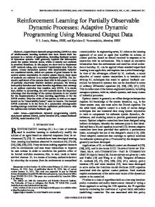
The evaluation domain used here is a grid world which consists of both smaller grid squares and the larger region squares which contain groups of grid squares. The region squares represent target areas to which the mobile robot must navigate. Using region squares for the agent’s goal rather than individual grid squares is preferable for our purposes, since the regions are intended to provide the basis for qualitative spatial reasoning in our system at a later date. There is only one active (i.e. goal) region square at any time, and whenever the robot enters the active region, it receives a reward, and a new goal region is chosen at random. The robot is situated in one of the grid squares, and faces in one of the four compass directions, north, east, south and west.
N
Region edges Grid squares Target region Robot
n g= 5 nr= 3
Fig. 1. An instance of the evaluation domain.
The simplicity of this domain makes it an ideal choice for illustration purposes. In addition, the size of the state space can be easily altered by changing the grid size, and planning knowledge can be incorporated in the form of high level movement operations. To evaluate performance as the state space is scaled-up, we define a class of these problems, where the regions are arranged in a square of side nr (see Figure 1). Each region contains a square set of grid squares, of side ng . Hence the size of the state space S, which encodes the position and direction of the robot, as well as the current destination region, is: |S| = 4n2g n4r
There are only three actions available to the robot: turn left, turn right and forward. Turn left turns the robot 90◦ anticlockwise to face a new compass direction. Turn right makes a 90◦ clockwise turn. Forward will move the robot one square forward in the current face direction, unless the robot is at the edge of the entire map of grid squares, in which case it has no effect. The robot receives a reward of 0 on every step, except on a step where the robot moves into the active region. When this happens, the robot receives a reward of 1 and a new active region is picked at random from the remaining regions. This introduces a small element of stochasticity to the domain, but this is not significant for the PLANQ-learner, since it will re-plan each time the goal (the active region) changes. The high level STRIPS representation of the evaluation domain abstracts away the state variables corresponding to the face direction of the robot and the position of the grid square it occupies in the current region. The representation is limited to reasoning at the region level, to plan a path between the current and target regions using a knowledge base which encodes an adjacency relation over the set of regions. Each region at a position (x, y) is represented as a constant r x y. The adj(r1,r2,dir) predicate encodes the fact that region r2 can be reached from region r1 by travelling in the direction dir, which can be one of the compass points N,S,E or W. The at(r) predicate is used to encode the current location of the robot, and to define the goal region to be reached. The operators available are NORTH, SOUTH, EAST and WEST, which correspond to low-level behaviours to be learned for moving in each of the four compass directions. The Planning Domain Definition Language [8] was used to pass data to the FF planner. An example of a planning problem in PDDL format is shown in Figure 2.
(:objects
r_0_0 r_0_1 r_1_0 r_1_1)
(:init
(adj r_0_0 r_1_0 (adj r_0_0 r_0_1 (adj r_0_1 r_1_1 (adj r_0_1 r_0_0 (adj r_1_0 r_0_0 (adj r_1_0 r_1_1 (adj r_1_1 r_0_1 (adj r_1_1 r_1_0 (at r_0_1))
(:goal
(at r_0_0)))
E) S) E) N) W) S) W) N)
Fig. 2. Part of the PDDL problem encoding for nr = 2.
nr = 3
ng = 5
nr = 5
ng = 5
0.1 Mean reward per step
Mean reward per step
0.2
0.15
0.1
Optimal Q-Learner PLANQ-Learner
0.05
0
0.08 0.06 0.04 Optimal Q-Learner PLANQ-Learner
0.02 0
0
0.5
1
1.5
2
2.5
3
Steps taken in the environment x 10-6
3.5
0
10
20
30
40
50
60
Steps taken in the environment x 10-6
Fig. 3. Results of Experiment 1: these graphs demonstrate that as larger values of nr are considered, the performance advantage of PLANQ-learning over Q-learning becomes progressively smaller.
7
Experiment 1: Results
In our first experiment, the PLANQ-learner was evaluated using a variety of values for nr and ng . For purposes of comparison, a standard Q-learning agent and an agent using a hand-coded version of the optimal policy were also evaluated in the domain. The standard Q-learner uses the full state space S as defined above, and chooses between the three low-level actions, turn left, turn right and forward. Like the PLANQ-learner, it receives a reward of 1 on a step where it enters a goal region, and a reward of 0 everywhere else. In all these experiments, the learning rate α is 0.1, the discount factor γ is 0.9, and the �-greedy parameter � is decayed linearly from 1.0 to 0.0 over the course of the experiment. We choose a decay rate for � such that any slower decay rate will not improve the quality of the solution. Examples of the performance of the agents over time are shown in Figure 3. The Q-learning agent consistently learns the true optimal policy. The PLANQlearner learns a good policy, but not quite the optimal one. This is because the planning model of the grid world does not model the cost of making turns - the plans {NORTH, EAST, NORTH, EAST} and {NORTH, NORTH, EAST, EAST} are considered equally suitable by the planner, but in reality the latter plan has a better reward rate. This results in slightly sub-optimal performance. In both of the experiments, the PLANQ-learner finds a good policy several times more quickly than the Q-learner. This is to be expected: the Q-learner must learn both high and low-level behaviours, whereas the PLANQ-learner need only learn the low-level behaviour. However it can be observed that the advantage of the PLANQ-learner over the Q-learner is less in the nr = 5 experiment than in the nr = 3 experiment. The general trend for the PLANQ-learner to lose advantage as nr increases is discussed in the next section.
8
Problems with Experiment 1
The learning speed-up achieved by the PLANQ-learner over the Q-learner can be attributed to the temporal abstraction inherent in the STRIPS formulation of the problem domain. The temporal abstraction allows us to express the overall problem as a number of sequential sub-problems, each of which is easier to learn than the overall task. Because the PLANQ-learner can learn the sub-tasks separately, it can finish learning more quickly than the Q-learner, which must tackle the problem as a whole. However, the advantage offered by temporal abstraction grows smaller as we scale up to larger domains because we have not supplied a state-abstraction to the PLANQ-learner. A state abstraction allows state variables to be excluded from the learner’s state space if they are not relevant to learning a particular task (or subtask). For instance, to learn the behaviour for the NORTH operator, only the direction and the position of the agent within the current region is relevant - the identities of the current and destination regions are irrelevant. Without the state abstraction, the PLANQ-learner has no way of knowing that the experience learned for moving NORTH from r0,1 to r0,0 can be exploited when moving from r2,1 to r2,0 (writing rx,y to represent the region at position (x, y) in the region grid). This means that the quality of a partially-learned operator can vary considerably in different regions of the grid world. The PLANQ-learner needs to perform enough exploration in the state space to learn the operator separately in all the regions in which it is applicable. As n r increases, the time taken to perform this exploration approaches the time taken by the Q-learner to learn the entire problem from scratch.
9
Adding State Abstraction
To exploit the STRIPS representation of PLANQ effectively, we incorporated a state abstraction mechanism into our system. Each of the STRIPS operators was annotated with the names of the state variables which were relevant for learning that operator (see bottom right of Figure 4). The Q-learner for that operator learns with a state space consisting only of these relevant variables. This speeds up learning by generalising the experience from one region to improve performance in another region. However, supplying this extra information to the PLANQ-learner gives it a significant advantage over the Q-learner, and comparing their learning times is unlikely to be useful. A more revealing comparison would be with a hierarchical Q-learner [1] which can take advantage of the temporal and state abstractions already exploited by PLANQ. We selected a hierarchical Q-learner based on the MAX-Q reward function decomposition [2]. The hierarchy used by the MAX-Q learner (see Figure 4) is based on four abstract actions corresponding to the STRIPS operators of PLANQ. The desired behaviour of each abstract action is determined by an internal reward function supplied as part of the hierarchy. The high-level task in the hierarchy is to find a
policy for executing the abstract actions to maximise the reward obtained from the environment. The hierarchy also encodes which state variables are relevant for learning each operator, and which state variables are relevant for learning the high-level policy for choosing abstract actions. Temporal Abstraction High−level control Policy for choosing abstract actions
North
West East
South
State Abstraction Relevant state variables Current region x−pos Current region y−pos Destination region x−pos Destination region y−pos
Relevant state variables Robot direction Robot x−offset within region Robot y−offset within region
Abstract actions
Fig. 4. Temporal and state abstractions used by MAX-Q.
10
Experiment 2: Results
Figure 5 shows the results obtained by the augmented PLANQ-learner and the MAX-Q learner for two instances of the evaluation domain. The PLANQ-learner consistently achieves a policy close to the optimal within a constant number of steps (around 100,000). Once it has learned a good policy for achieving each of the operators in an arbitrary 5x5 region (thanks to the state abstraction), the PLANQ-learner has enough information to achieve a good rate of return in a region square of arbitrary size. In other words, the number of steps needed for the PLANQ-learner to achieve a good rate of return is dependent only on ng , not on nr . The MAX-Q learner on the other hand needs to learn both the low-level abstract actions and the high-level policy for choosing abstract actions. By exploiting both this temporal abstraction and the state abstraction information supplied with the hierarchy, the MAX-Q learner can achieve a hierarchicallyoptimal policy [2] in orders of magnitude less time than the original Q-learner takes to achieve a good rate of return. However, the number of steps the MAX-Q learner needs to achieve this policy does increase with nr , since the high-level policy becomes more difficult to learn. So as the value of nr is increased, the PLANQ-learner outperforms MAX-Q to a greater degree.
nr = 4
ng = 5
nr = 6 0.07
0.1 0.08 0.06 0.04 0.02
ng = 5
0.08 Mean reward per step
Mean reward per step
0.12
Optimal MAX-Q PLANQ + Abstraction
0.06 0.05 0.04 0.03 Optimal MAX-Q PLANQ + Abstraction
0.02 0.01
0
0 0 0.05 0.1 0.15 0.2 0.25 0.3 0.35 0.4
0
Steps taken in the environment x 10-6
0.1
0.2
0.3
0.4
0.5
0.6
0.7
Steps taken in the environment x 10-6
Fig. 5. Results of Experiment 2: The PLANQ learner using state abstraction consistently learns a near-optimal policy in around 105 time steps as we increase the value of nr . In contrast, the MAX-Q learner takes an increasing number of time steps to learn a policy of similar quality as nr is increased.
11
Computational Requirements
Although PLANQ achieved a good policy after fewer actions in the environment than the other agents, it is important to consider the CPU time required to calculate each action choice. Our original implementation used the FF planner and the STRIPS encoding shown in Figure 2. This scaled very poorly in terms of CPU time - we could only obtain results for nr ≤ 6. To improve the scaling properties of PLANQ, we implemented our own version of a Graphplan planner, eliminating costly operations such as parsing and file-access, but still providing a fully functional domain-independent planner.
(:objects
n0 n1 n2)
(:init
(s (s (x {y
n0 n1) n1 n2) n0) n0))
(:goal
(x n1) (y n2)))
Fig. 6. Alternative PDDL problem encoding for nr = 3.
We also adopted an alternative STRIPS encoding of the evaluation domain, shown in Figure 6. This involves encoding a subset of the natural numbers with the successor relation s(a,b), and representing the x and y coordinates inde-
pendently as x(n) and y(n). Replacing the adjacency relation with a successor relation means that the number of formulae in the initial conditions is O(n r ) instead of O(n2r ), which makes a great improvement to the performance of PLANQ. Figure 7 shows the amount of CPU time taken for PLANQ to learn a policy with 95% optimal performance. While the MAXQ learning method is infeasible for nr > 20, PLANQ can learn to make near-optimal action choices in under a minute while nr < 50. However, as nr approaches 70, PLANQ also starts to become infeasible.
CPU Time (seconds)
200
PLANQ MAXQ
150
100
50
0 0
10
20
30
40
50
60
70
nr
Fig. 7. CPU time required to achieve 95% optimal performance when ng = 5.
A key limitation of the PLANQ algorithm in its current form is the large variance in CPU time required per time step. On most steps an action choice can be made in a few microseconds, but if the planner needs to be invoked the choice may be delayed for 50 or 100 milliseconds. For systems with real-time constraints this is clearly unacceptable, and we plan to address this problem in future research.
12
Conclusions and Related Work
In this series of experiments, we have shown that an AI planning algorithm based on the STRIPS representation can be combined successfully with reinforcement learning techniques, resulting in an agent which uses an explicit symbolic description of its prior knowledge of a learning problem to constrain the number of action steps required to learn a policy with a good (but not necessarily optimal) rate of return. The STRIPS representation used in this work is limited to describing problems which are deterministic, fully observable, and goal oriented. To overcome
some of these limitations, the PLANQ method could be adapted to use a more complex planner which can reason about stochastic action effects and plan quality. However, we believe that prior knowledge encoded in the limited STRIPS representation will still be useful for speeding up the learning of many problems, even if some aspects of those problems are inexpressible in the representation. Our technique for deriving a reward function from the pre-conditions and effects of a STRIPS operator is similar to that used by Ryan [9], although his work is primarily concerned with teleo-reactive planning in contrast to the classical STRIPS plans used in our work. Boutilier et al. [10] employ symbolic plans to solve factored MDPs with reward functions expressible as an additive combination of sub-goals. Partiallyordered plans are used as an intermediate representation for constructing a high quality solution which makes a trade-off between the sub-goals.
References 1. Barto, A., Mahadevan, S.: Recent advances in hierarchical reinforcement learning. Discrete Event Systems 13 (2003) 41–77 2. Dietterich, T.G.: Hierarchical reinforcement learning with the MAXQ value function decomposition. Journal of Artificial Intelligence Research 13 (2000) 227–303 3. Watkins, C.J.C.H.: Learning from Delayed Rewards. PhD thesis, Cambridge University, U.K. (1989) 4. Fikes, R., Nilsson, N.: STRIPS: A new approach to the application of theorem proving to problem solving. Artificial Intelligence 2 (1971) 189–208 5. Blum, A.L., Furst, M.L.: Fast planning through planning graph analysis. Artificial Intelligence 90 (1997) 281–300 6. Hoffmann, J.: A heuristic for domain independent planning and its use in an enforced hill-climbing algorithm. In: Proceedings of the 12th International Symposium on Methodologies for Intelligent Systems. (2000) 216–227 7. Bertsekas, D.P., Tsitsiklis, J.N.: Neuro-Dynamic Programming. Athena Scientific (1996) 8. Ghallab, M., Howe, A., Knoblock, C., McDermott, D., Ram, A., Veloso, M., Weld, D., Wikins, D.: PDDL—the planning domain definition language. Technical Report CVC TR-98-003/DCS TR-1165, Yale Center for Computational Vision and Control (1998) 9. Ryan, M.: Using abstract models of behaviours to automatically generate reinforcement learning hierarchies. In: Proceedings of the 19th International Conference on Machine Learning. (2002) 10. Boutilier, C., Brafman, R.I., Geib, C.: Prioritized goal decomposition of Markov decision processes: Towards a synthesis of classical and decision theoretic planning. In: International Joint Conference on Artificial Intelligence. (1997)