Combining Visual Attention, Object Recognition and Associative

Combining Visual Attention, Object Recognition and Associative Information Processing in a NeuroBotic System Rebecca Fay, Ulrich Kaufmann, Andreas Knoblauch, Heiner Markert, and G¨ unther Palm University of Ulm, Department of Neural Information Processing, D-89069 Ulm, Germany

Abstract. We have implemented a neurobiologically plausible system on a robot that integrates visual attention, object recognition, language and action processing using a coherent cortex-like architecture based on neural associative memories. This system enables the robot to respond to spoken commands like ”bot show plum” or ”bot put apple to yellow cup”. The scenario for this is a robot close to one or two tables carrying certain kinds of fruit and other simple objects. Tasks such as finding and pointing to certain fruits in a complex visual scene according to spoken or typed commands can be demonstrated. This involves parsing and understanding of simple sentences, relating the nouns to concrete objects sensed by the camera, and coordinating motor output with planning and sensory processing.

1

Introduction

Detecting and identifying objects as well as processing language and planning actions are essential skills for robots performing non-trivial tasks in real world environments. The combination of object recognition, language understanding and information processing therefore plays an important role when developing service robots. We have implemented a neurobiologically inspired system on a robot that integrates visual attention, object recognition, language and action processing using a coherent cortex-like architecture based on neural associative memories (cf. [1]). Neural networks and associative memories which are both neurobiologically plausible and fault tolerant form the basic components of the model. The model is able to handle a scenario where a robot is located next to one or two tables with different kinds of fruit and other simple objects on them (cf. figure 4). The robot (”bot”) is able to respond to spoken commands such as ”bot show plum” or ”bot put apple to yellow cup” and to perform tasks like finding and pointing to certain fruits in a complex visual scene according to a spoken or typed command. This involves parsing and understanding of simple sentences, relating the nouns to concrete objects sensed by the camera, and coordinating motor output with planning and sensory processing. S. Wermter et al. (Eds.): Biomimetic Neural Learning, LNAI 3575, pp. 117–142, 2005. c Springer-Verlag Berlin Heidelberg 2005

118

R. Fay et al.

The underlying cortical architecture is motivated by the idea of distributed cell assemblies in the brain [2][3]. For visual preprocessing we use hierarchically organized radial-basis-function networks to classify objects selected by attention, where hidden states in this hierarchical network are used to generate sparse distributed cortical representations. Similarly, auditory input pre-processed by standard Hidden-Markov-Model architectures can be transformed into a sparse binary code for cortical word representations. In further cortical areas for language and action the sensory input is syntactically and semantically interpreted and finally translated into motor programs. The essential idea behind the cortical architecture is that different cortical areas represent different aspects (and correspondingly different notions of similarity) of the same entity (e.g., visual, auditory language, semantical, syntactical or grasp-related aspects of an apple) and that the (mostly bidirectional) long-range cortico-cortical projections represent hetero-associative memories that translate between these aspects or representations. These different notions of similarity can synergistically be used, for example, to resolve ambiguities within or across sensory modalities.

2

Architecture

Our architecture can roughly be divided into two large parts: (1) Sensory preprocessing and (2) cortical model. In the preprocessing part features are extracted from auditory and visual input selected by attention control. For the cortical model several different neural architectures are used. For object recognition and speech processing more artificial neural networks such as radial-basis-function networks are utilized, while a biologically more plausible architecture of many interconnected neural associative memories is used to model cortical information processing. Figure 1 shows the different components of our model, their interactions and the division into two parts. For the implementation of cortical cell assemblies [4][5][6][7][8][9], we decided to use the Willshaw model of associative memory as an elementary architectural framework. A cortical area consists of n binary neurons which are connected with each other by binary synapses. A cell assembly or pattern is a sparse binary vector of length n where k one-entries in the vector correspond to the neurons belonging to the assembly. Usually k is much smaller than n. Assemblies are represented in the synaptic connectivity such that any two neurons of an assembly are bidirectionally connected. Thus, an assembly consisting of k neurons can be interpreted as a k-clique in the graph corresponding to the binary matrix A of synaptic connections. This model class has several advantages over alternative models of associative memory such as the most popular Hopfield model [10]. For example, it better reflects the cortical reality where it is well known that activation is sparse (most neurons are silent most of the time), and that any neuron can have only one type of synaptic connection (either excitatory or inhibitory). Instead of classical one-step retrieval we used an extended algorithm based on spiking associative memory [11][12]. A cortical area is modeled as a local neuron population which receives input from other areas via hetero-associative Hebbian

Combining Visual Attention, Object Recognition and Associative Information

119

Fig. 1. The architecture is roughly divided into two parts: Sensory preprocessing and cortical model

Fig. 2. Interaction of the different areas of the cortical model (v : visual, l : location, f : contour features, o: visual objects, h: haptic / proprioceptive, p: phonetics, s: syntactic, a: action / premotoric, g: goals / planning) and their rough localization in the human brain

synaptic connections. In each time step this external input initiates pattern retrieval. The neurons receiving the strongest external input will fire first, and all emitted spikes are fed back immediately through the auto-associative Hebbian synaptic connections which allows both the activation of single assemblies and the representation of superpositions. In comparison to the classical model, this model has a number of additional advantages. For example, assemblies of dif-

120

R. Fay et al.

Fig. 3. Cortical architecture involving several inter-connected cortical areas corresponding to auditory, grammar, visual, goal, and motor processing. Additionally the model comprises evaluation fields and activation fields (see text)

ferent size k can be stored, input superpositions of several assemblies can more easily be separated, and it is possible to transmit more subtle activation patterns (e.g., about ambiguities or superpositions) in the spike timing. As already shown in figure 1, our cortical model divides into four main parts. Some of those again are quite complex tasks that may, considering the situation in the human brain, involve some different cortical areas. In figure 2, a rough overview of the cortical areas that are somehow reflected in our system is given. The interconnections shown there correspond to the flow of information we realized in our model. Figure 3 illustrates the overall architecture of our cortical model. Each box corresponds to a local neuron population implemented as spiking associative memory. The model consists of phonetic auditory areas to represent spoken language, of grammar related areas to interpret spoken or typed sentences, visual areas to process visual input, goal areas to represent action schemes, and motor areas to represent motor output. Additionally, we have auxiliary areas or fields to activate and deactivate the cortical areas (activation fields), to compare corresponding representations in different areas (evaluation fields), and to direct visual attention. The primary visual and auditory areas are part of sensory preprocessing and comprise additional (artificial) neural networks for processing of camera images and acoustic input. The suggested approach is implemented on the PeopleBot base by ActivMedia. To integrate the implemented functionality on the robot we used Miro [13], a robot middleware framework that allows control of the robot’s hardware and facilitates communication with other programs by using Corba. Miro supports distributed computing, i.e. time consuming calculations with low i/o-rates can be outsourced to other computers. Miro also facilitates the usage of the same application on different robot platforms. Hence the software developed here runs on the PeopleBot as well as on other robot bases.


121

Fig. 4. In the test scenario the robot is situated in front of a table. Different objects are laying on this table. The robot has to grasp or point to specified objects

3

Sensory Preprocessing

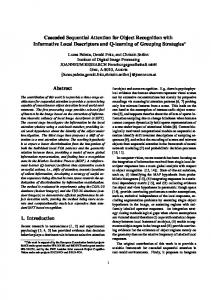
The object classification is performed in three stages, i.e. the system consists of three components which are activated consecutively. First objects of interests are to be localized within the robot’s camera image. Since neither the camera image contains solely the object of interest but also background as well as possible other objects nor is it guaranteed that the object is located in the center of the image, it is necessary to perform a pre-processing of the image. In the course of this preprocessing a demarcation of the objects from the background and from each other as well as a localization of the objects takes place. For this a color-based visual attention control algorithm is used to find regions of interests within the camera images. These regions contain objects to be classified. Once the objects are localized, characteristic features like orientation histograms or color information are extracted, which should be invariant to lighting conditions. In order to save computing time the features are not extracted from the entire image but only from the region of interest containing the object. These features are used to classify the localized objects one after the other. Due to the fact that the objects are centered within the regions of interest, the extracted features are made shift and scaling invariant. This yields improved classification results. The fact that in a first step meaningful objects are separated from meaningless background further improves the classification. Moreover, this accounts for invariance of the classification regarding background conditions. An overview of the whole process is shown in figure 5.

122

R. Fay et al.

Fig. 5. The classification system consists of three components arranged in successive order: object localization, feature extraction and classification. The figure depicts the interconnections as well as the inputs and outputs of the miscellaneous components. Starting with the robot’s camera image the classification process is shown. The attentional system currently works on visual sensory input. In the first step, the camera image is searched for regions containing interesting low level features (e.g., blobs of desired color). In the second step, additional features are extracted from the region of interest to be used by the object recognition system

3.1

Attentional System

The attentional system [14] receives input from some higher goal and motor areas which specify the current interest of the robot (e.g., searching for redcolored objects; areas M2 or M2attr in Fig. 3). Subsequently, the camera image is processed by standard computer vision algorithms in order to find regions of interest (see Fig. 5). If an interesting region is found, this part of the image is analyzed in more detail. Features (e.g., orientation histograms) are extracted and transmitted to the object recognition system which is explained in detail in the next section. The object recognition system classifies the object in the region of interest and transmits the information to the corresponding visual cortical area (areas V2 and V2attr). After some time, attention shifts to the next region of interest, until this process is interrupted by a cortical area controlling attention (e.g., areas G1 and M1). When locating relevant objects in complex visual scenes it would be too time-consuming to simply look at all possible regions. Therefore pre-processing

Fig. 6. Meaningful objects are separated from the background and are marked as regions of interest. The object colour is used to identify objects of interest. This also allows to detect partially occluded objects


123

is necessary to segment the image into interesting and non interesting regions. To reduce the time expense of the following process steps the number of regions that do not contain a relevant object should be minimized. It also should be ensured that all regions that contain a relevant object will be detected in this step. This pre-processing which separates meaningful objects from the background is called visual attention control which defines rectangular regions of interest (ROI). A region of interest is defined herein as the smallest rectangle that contains one single object of interest. Figure 6 shows the process of placing the region of interest. Especially in the field of robotics real-time requirements have to be met, i.e. a high frame processing rate is of great importance. Therefore the usage of simple image processing algorithms is essential here. The attention control algorithm consists of six consecutive steps. Figure 7 shows the intermediate steps of the attention control algorithm. Camera images in the RGB format constitute the starting point of the attention control algorithm. At first the original image is smoothed using a 5 × 5 Gaussian filter. This also reduces the variance of colors within the image. The smoothed image is then converted to HSV color space, where color information can be observed independent of the influence of brightness and intensity. In the following only the hue components are considered. The next step is a color clustering. For this purpose the color of the object of interest and a tolerance are specified. The HSV image is searched for colors falling into this predefined range. Thereafter the mean hue value of the so identified pixels is calculated. This mean value together with a predefined tolerance is now used to once again search for pixels with colors in this new range. The result is a binary image where all pixels that fall into this color range are set to black and all others are set to white. Owing to this adaptivity object detection is more robust against varying lighting conditions. The results are further improved using the morphological closing operation [15]. The closing operation has the effect of filling-in holes and closing gaps. In a last

Fig. 7. The intermediate steps of the attention control algorithm

124

R. Fay et al.

step a floodfill algorithm [16] is applied to identify coherent regions. The region of interest is then determined by the smallest rectangle that completely encloses the region found. Simple heuristics are used to decide whether such a detected region of interest contains an object or not. For the problem at hand the widthto-height ratio of the region of interest as well as the ratio of pixels belonging to the object to pixels belonging to the background in the region of interest are determined. This method allows for detecting several objects in one scene and can handle partial occlusion to a certain degree. 3.2

Feature Extraction

Simply using the raw image data for classification would be too intricate. Furthermore dispensable and irrelevant information would be obtained. Therefore it is necessary to extract characteristic features from the image which are suitable for classification. These features are more informative and meaningful for they contain less redundant information and are of a lower dimensionality than the original image data. To reduce calculation time, features will be extracted from the detected regions of interest only. Thus even expensive image processing methods can be used to calculate the features. If the object was localized precisely enough this yields translation and partial scaling invariance. The selection of the features depends, inter alia, on the objects to be classified. For the distinction of different fruits, appropriate features are those representing color and form of the object present. Among others we use the mean color values of the HSV representation of the detected region of interest as well as orientation histograms [17] summing up all orientations (directions of edges represented by the gradient) within the region of interest. To determine the mean color values the camera image is converted from RGB color space to HSV color space [18]. For each color channel the mean value of the localized object within the region of interest is calculated. Color information is helpful to distinguish e.g. between green and red apples. Advantages of color information are its scale and rotation invariance as well as its robustness to partial occlusion. Furthermore it can be effectively calculated. To calculate the orientation histograms which represent the form of the object the gradient in x and y direction of the grey value image is calculated using the Sobel edge detector [19]. The gradient angles are discretized. Here we divided the gradient angle range into eight sections. The discrete gradient directions are weighted with the gradient value and summed to form the orientation histogram. The orientation histogram provides information about the directions of the edges and their intensity. It has been found that the results achieved could be improved if not only one orientation histogram per region of interest is used to represent the form of the object but several orientation histograms are calculated from different parts of the region of interest as information about the location of the orientations is not completely disregarded. The region of interest is therefore split into m × m parts of the same size. For each part a separate orientation histogram is calculated. The concatenated orientation histograms then form the feature vector. If the


125

Fig. 8. The image is split into sub-images. For each sub-image an orientation histogram is calculated by summing up the orientations that occur in this sub-image. For reasons of simplicity non-overlapping sub-images are depicted

parts overlap by about 20% the result improves further since it becomes less sensitive to translation and rotation. We chose to divide the image into 3 × 3 parts with approximately 20% overlap. Figure 8 illustrates how an orientation histogram is generated. The dimension of the feature vector depends only on the number of subimages and the number of sections used to discretise the gradient angle. The orientation histogram is thus largely independent of the resolution of the image used to extract the features.

4

Cortical Model

Our cortical model consists of four parts, namely speech recognition, language processing, action planning and object recognition (see also figure 1). For speech recognition standard Hidden-Markov-Models on single word level are used, but for simplicity it is also possible to type the input directly via a computer terminal. The resulting word stream serves as input to the language processing system, which analyzes the grammar of the stream. The model is capable of identifying regular grammars. If a sentence is processed which is incorrect with respect to the learned grammar, the systems enters an error state, otherwise, the grammatical role of the words is identified. If the sentence is grammatically interpreted, it becomes possible to formulate what the robot has to do, i.e. the goal of the robot. This happens in the action planning part, which receives the corresponding input from the language processing system. The robot’s goal (e.g. ”bot lift plum”) is then divided into a sequence of simple subgoals (e.g. ”search plum”, ”lift plum”) necessary to archive the goal. The action planning part initiates and controls the required actions to archive each subgoal, e.g. for ”search red plum”, the attentional system will be told to look for red objects. The detected areas of interest serve as input for the object recognition system, the fourth part of our cortical model.

126

R. Fay et al.

We use hierarchically organized RBF (radial basis function) networks for object recognition, which are more accurate compared to a single RBF network, while still being very fast. The output of the object recognition again serves as input to the action planning system. If in our example a plum is detected, the action planning areas will recognize that and switch to the next subgoal, which here would be to lift the plum. The language as well as the action planning part are using the theory of cell assemblies which is implemented using Willshaw’s model of associative memory [4][5][6][7][8][9]. This results in an efficient, fault tolerant and still biological realistic system. 4.1

Visual Object Recognition

The visual object recognition system is currently implemented using a hierarchical arrangement of radial-basis-function (RBF) networks. The basic idea of hierarchical neural networks is the division of a complex classification task into several less complex tasks by making coarse discrimination at higher levels of the hierarchy and refining the discrimination with increasing depth of the hierarchy. The original classification problem is decomposed into a number of less extensive classification problems organized in a hierarchical scheme. Figure 9 shows a hierarchy for recognition of fruits and gestures which has been generated by unsupervised k-means clustering. From the activation of the RBF networks (the nodes in Fig. 9) we have designed a binary code in order to express the hierarchy into the domain of cell assemblies. This code should preserve similarity of the entities as expressed by the hierarchy. A straightforward approach is to use binary vectors of length corresponding to the total number of neurons in all RBF networks. Then in a representation of a camera image those components are activated that correspond to the l strongest activated RBF cells on each level of the hierarchy. This results in sparse and translation invariant visual representations of objects. That way, the result of the object recognition is transformed into the binary code, and using additional information about space and location from the attentional system, the corresponding neurons are activated in areas V1,V2,V2attr, and V3. Hierarchical Neural Networks. Neural networks are used for a wide variety of object classification tasks [20]. An object is represented by a number of features, which form a d dimensional feature vector x within the feature space X ⊆ IRd . A classifier therefore realizes a mapping from feature space X to a finite set of classes C = {1, 2, ..., l}. A neural network is trained to perform a classification task using supervised learning algorithms. A set of training examples S := {(xµ , tµ ), µ = 1, ..., M } is presented to the network. The training set consists of M feature vectors xµ ∈ IRd each labeled with a class membership tµ ∈ C. During the training phase the network parameters are adapted to approximate this mapping as accurately as possible. In the classification phase unlabeled data


127

xµ ∈ IRd are presented to the trained network. The network output c ∈ C is an estimation of the class corresponding to the input vector x. The basic idea of hierarchical approaches to object recognition is the division of a complex classification task into several smaller and less complex ones [21]. The approach presented here hierarchically decomposes the original classification problem into a number of less extensive classification problems. Starting with coarse discriminations between few (but large) subsets of classes at higher levels of the hierarchy the discriminations are stepwise refined. At the lowest levels of the hierarchy there are discriminations between single classes. Thus the hierarchy emerges from successive partitioning of sets of classes into disjoint subsets, i.e the original set of classes is recurrently decomposed into several disjoint subsets until subsets consisting of single elements result. This leads to a decrease in the number of class labels processed in a decision node with increasing depth of this node. The hierarchy consists of several simple neural networks that are stratified as a tree or more generally as a rooted directed acyclic graph, i.e. each node within the hierarchy represents a neural network that works as a classifier. The division of the complex classification problem into several less complex classification problems entails that instead of one extensive classifier several simple classifiers are used which are more easily manageable. This has not only a positive effect on the training effort, but also simplifies modifications of the design since the individual classifiers can be amended much more easily to the decomposed simple classification problems than one classifier could be adapted to a complex classification task. The use of different feature types additionally facilitates the classification tasks at different nodes, since for each classification task the feature type that allows for the best discrimination can be chosen. Hence for each data point within the training set a feature vector for each prototype is available. Moreover the hierarchical decomposition of the classification result provides additional intermediate information. In order to solve a task it might be sufficient to know whether the object to be recognized belongs to a set of classes and the knowledge of the specific category of the object might not add any value. The hierarchy also facilitates a link between symbolic information and subsymbolic information: The classification itself is performed using feature vectors which represent sub-symbolic information, whereas symbolic knowledge can be provided concomitantly via the information about the affiliation to certain subsets of classes. The usage of neural networks allows the representation of uncertainty of the membership to these classes since the original output of the neurons is not discrete but continuous. Moreover a distributed representation can easily be generated from the neural hierarchy. Since the hierarchy is generated using features which are based on the appearance of the objects such as orientation or color information it primarily reflects visual similarity. Thus it allows the generation of a sparse similarity preserving distributed representation of the objects. A straight-forward approach is the usage of binary vectors of length corresponding to the total number of neurons in the output layer of all networks in the hierarchy. The representation is created identifying the strongest

128

R. Fay et al.

activated output neurons for each node. The corresponding elements of the code vector are then set to 1, the remaining elements are set to 0. These properties are extremely useful in the field of neuro-symbolic integration [22] [23] [24]. For separate object localization and recognition a distributed representation may not be relevant, but in the overall system in the MirrorBot project this is an important aspect [25]. Hierarchy Generation. The hierarchy is generated by unsupervised k-means clustering [26]. In order to decompose the set of classes assigned to one node into disjoint subsets a k-means clustering is performed with all data points belonging to these classes. Depending on the distribution of the classes across the k-means clusters disjoint subsets are formed. One successor node corresponds to each subset. For each successor node again a k-means clustering is performed to further decompose the corresponding subset. The k-means clustering is performed for each feature type. Since the k-means algorithm depends on the initialization of the clusters, k-means clustering is performed several times per feature type. The number of clusters k must be at least the number of successor nodes or the number of subsets respectively but can also exceed this number. If the number of clusters is higher than the number of successor nodes, several clusters are grouped together so that the number of groups equals the number of successor nodes. All possible groupings are evaluated. In the following all equations only refer to clusterings for reasons of simplicity, i.e. the number of clusters k equals the number of successor nodes. A valuation function is used to rate the clusterings or groupings respectively. The valuation function prefers clusterings that group data according to their class labels. Clusterings where data are uniformly distributed across clusters notwithstanding their class labels receive low ratings. Furthermore clusterings are preferred which evenly divide the classes. Thus the valuation function rewards unambiguity regarding the class affiliation of the data assigned to a prototype as well as uniform distribution regarding the number of data points assigned to each prototype. The valuation function V (p) consists of two terms regulated by a scaling parameter λ > 0. The first term E(p) calculates the entropy of the distribution of each class across the different clusters. This accounts for unambiguous distribution of the data considering the corresponding classes. The term E(p) becomes minimal if it is ensured for all classes that all data belonging to one class is assigned to one cluster. It becomes maximal if all data belonging to one class is uniformly distributed across all clusters. The second term D(p) computes the deviation from the uniform distribution. This term becomes minimal if each cluster is assigned the same number of data points. This allows for the even division of the classes into subsets. During the hierarchy generation phase we are looking for clusterings that minimize the valuation function V (p). The influence of the respective term is regulated by the scaling parameter λ. Both terms are normalized so that they return values of the interval [0, 1]. The valuation function V (p) is given by V (p) =

1 1 E(p) + λ D(p) → min l log2 (k) l(k − 1)


where E(p) = pji

Pl

i=1 (−

Pk

j j=1 (pi

log2 (pji ))), D(p) =

Pk

j=1

|

Pl

i=1

pji −

129 l k|

and

|Xi ∩Zj | |Xi |

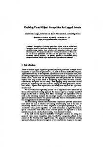
= denotes the rate of patterns from class i, that belong to cluster j. Here Xi = {xµ |µ = 1, ..., M ; tµ = i} ⊆ X is the set of data points that belong to class i, Rj = {x ∈ IRd |j = argminTi=1,...,k kx − zi k} denotes the Voronoi cell [27] defined by cluster j and Zj = Rj X is the set of data points that were assigned to cluster j. zi is the center of cluster i. The best clustering, i.e. the one that minimizes the valuation function V (p), is chosen and is used for determining the division of the set of classes into subsets. Moreover this also determines which feature type will be used to train the corresponding classifier. So each classifier within the hierarchy can potentially use a different feature type and thereby operates in a different feature space. To identify which classes will be added to which subset the distribution of the data across the clusters is considered. The division in subsets Cj is carried out by maximum detection. The set of classes belonging to subset Cj is defined as Cj = {i ∈ C|j = argmax{qi,1 , ..., qi,k }} |Xi ∩Zj | denotes the rate of class i in cluster j. For each class it where qi,j = |Z j| is determined to which cluster the majority of data points belonging to this class were associated. The class label will then be added to the corresponding subset. To generate the hierarchy at first the set of all classes is assigned to the root node. Starting with a clustering on the complete data set the set off classes is divided into subsets. Each subset is assigned to a successor node of the root node. Now the decomposition of the subsets is continued until no further decomposition is possible or until the decomposition does not lead to a new division. An example of a classification hierarchy is shown in figure 9.

Fig. 9. Classifier hierarchy generated for the classification of different kind of fruits using two feature types: orientation histograms and color information. Each node within the hierarchy represents a neural network or a classifier respectively. The end nodes represent classes. To each node a feature type and a set of classes is assigned. The corresponding neural network uses the assigned feature type to discriminate between the assigned classes

130

R. Fay et al.

Training and Classification. Within the hierarchy different types of classifiers can be used. Examples of classifiers would be radial basis function (RBF) networks, linear vector quantization classifiers or support vector machines. We chose RBF networks [28] as classifiers. They were trained with a three phase learning algorithm [29]. The hierarchy is trained by separately training each neural network within the hierarchy. The classifiers are trained using supervised learning algorithms. Each classifier is trained only with data points belonging to the classes assigned to the corresponding node hence the complete training set is only used to train the classifier that represents the hierarchy’s root node. The classifiers are trained with the respective feature type identified during the hierarchy generation phase. To train the classifiers the data will be relabeled so that all data points of the classes that belong to one subset have the same label. The classifiers within the hierarchy can be trained independently, i.e. all classifiers can be trained in parallel. The classification result is retrieved similar to the retrieval in a decision tree [27]. Starting with the root node the respective feature vector of the object to be classified is presented to the trained classifier. By means of the classification result the next classifier to categorize the data point is determined. Thus a path through the hierarchy from the root node to an end node is obtained which not only represents the class of the object but also the subsets of classes to which the object belongs. Hence the data point is not presented to all classifier within the hierarchy. If only intermediate results are of interest it is not necessary to evaluate the complete path. 4.2

Language Processing System

Our language system consists of a standard Hidden-Markov-based speech recognition system for isolated words and a cortical language processing system which can analyze streams of words detected with respect to simple (regular) grammars. For simplicity, the speech recognition system can also be replaced by direct text input via a computer terminal and a wireless connection to the robot. Regular Grammars, Finite Automata and Neural Assemblies. Regular grammars can be expressed by generative rules of the type A 7→ a or A 7→ bC, where capital letters are variables and lower case letters are terminal symbols, i.e. elements in of an alphabet Σ. There is usually a special starting variable S which can be expanded by applying the rules. Let Σ ∗ be the set of all possible strings of symbols from the alphabet Σ with arbitrary length. A sentence s ∈ Σ ∗ is then called valid with respect to the grammar, if it can be derived from S by applying the grammatical rules and resolving all variables by terminal symbols. It is easy to show that regular grammars are equivalent to deterministic finite automata. A deterministic finite automate (DFA) can be specified by the set M = (Z, Σ, δ, z0 , E), where Z = {z0 , z1 , . . . , zn } is a finite set of states, Σ is the alphabet, z0 ∈ Z is the starting state and E ⊆ Z contains the terminal states.


131

Fig. 10. Comparison of deterministic finite automate (DFA, left side) with a neural network (middle) and cell assemblies (right). Each δ-transition δ(zi , ak ) = zj corresponds to synaptic connections from neuron Ci to Cj and from input neuron Dk to Cj in the neural network. For cell assemblies, the same basic architecture as for the neural net (lower part in the middle) is used, but instead of using single neurons for the states, assemblies of several cells are used

Finally, the function δ : (Z, Σ) → Z defines the state transitions. A sentence s = s1 s2 . . . sn ∈ Σ ∗ is valid with respect to the DFA, if iterated application of δ on z0 and the letters of s transfers the automates starting state z0 into one of the terminal states in E, i.e. if δ(. . . δ(δ(z0 , s1 ), s2 ), . . . , sn ) ∈ E. We now show that DFAs can easily be modelled by recurrent neural networks. For an overview, see also figure 10. This recurrent binary network is specified by N = (C, D, W, V, C1 ), where C = (C1 , C2 , . . . , Cn ) contains the local cells of the network, D = (D1 , D1 , . . . Dm ) is the set of external input cells, C1 is the starting neuron and W = (wij )n×n as well as V = (vij )m×n are binary matrices. Here, wij describes the strength of the local synaptic connection between neuron Ci and neuron Cj , where vij is the synaptic strength between neuron Di and neuron Cj . The network evolves in discrete time steps, where a neuron Ci is activated if the sum over its inputs exceeds threshold Θi , otherwise, it is inactive, i.e. P P 0 , if j wji Cj (t) + j vji dj (t) ≥ Θi . Ci (t + 1) = 1 , otherwise To simulate a DFA, we need to identify the alphabet Σ with the external input neurons D and the states Z with the local cells C. The synapses wij and vk j are active if and only if δ(zi , ak ) = zj for the transition function δ of the DFA. Finally, set all thresholds Θi = 1, 5 and activate only the starting neuron D0 at time 0. A sentence s = s1 s2 . . . sn is then presented by activating neuron Dst at the discrete time t ∈ {1, . . . , n} and to deactivate all other neurons Dj with j 6= st . Then, the network simulates the DFA, i.e. after presenting the last symbol of the sentence, one of the neurons corresponding to the terminal states of the DFA will be active if and only if the sentence was valid with respect to the simulated DFA. Biologically, it would be more realistic to have cell assemblies (i.e. strongly interconnected group of nearby neurons) representing the different states. This

132

R. Fay et al.

Fig. 11. The language system consisting of 10 cortical areas (large boxes) and 5 thalamic activation fields (small black boxes). Black arrows correspond to inter-areal connections, gray arrows within areas correspond to short-term memory

enables fault tolerance, since incomplete input can be completed to the whole assembly, furthermore, it becomes possible to express similarities between the represented objects via overlaps of the corresponding assemblies. Cell Assembly Based Model. Figure 11 shows 15 areas of our model for cortical language processing. Each of the areas is modeled as a spiking associative memory of 400 neurons. Similar as described for visual object recognition, we a priori defined for each area a set of binary patterns constituting the neural assemblies stored auto-associatively in the local synaptic connections. The model can roughly be divided into three parts. (1) Primary cortical auditory areas A1, A2, and A3: First, auditory input is represented in area A1 by primary linguistic features (such as phonemes), and subsequently classified with respect to function (area A2) and content (area A3). (2) Grammatical areas A4, A5-S, A5-O1-a, A5O1, A5-O2-a, and A5-O2: Area A4 contains information about previously learned sentence structures, for example that a sentence starts with the subject followed by a predicate (see Fig. 12). In addition to the auto-associative connections, area A4 has also a delayed feedback-connection where the state transitions are stored hetero-associatively. The other grammar areas contain representations of the different sentence constituents such as subject (A5-S), predicate (A5-P), or object (A5-O1, O1-a, O2, O2-a). (3) Activation fields af-A4, af-A5-S, afA5-O1, and af-A5-O2: The activation fields are relatively primitive areas that are connected to the corresponding grammar areas. They serve to activate or deactivate the grammar areas in a rather unspecific way. Although establishing a concrete relation to real cortical language areas of the brain is beyond the scope


133

Fig. 12. Graph of the sequence assemblies in area A4. Each node corresponds to an assembly, each arrow to a hetero-associative link, each path to a sentence type. For example, a sentence “Bot show red plum” would be represented by the sequence (S,Pp,OA1,O1,ok SPO)

of this work [30][31], we suggest that areas A1,A2,A3 can roughly be interpreted as parts of Wernicke’s area, and area A4 as a part of Broca’s area. The complex of the grammatical role areas A5 might be interpreted as parts of Broca’s or Wernicke’s area, and the activation fields as thalamic nuclei. 4.3

Planning, Action and Motor System

Our system for cortical planning, action, and motor processing can be divided into three parts (see Fig. 13). (1) The action/planning/goal areas represent the robot’s goal after processing a spoken command. Linked by hetero-associative connections to area A5-P, area G1 contains sequence assemblies (similar to area A4) that represent a list of actions that are necessary to complete a task. For example, responding to a spoken command “bot show plum” is represented by a sequence (seek,show), since first the robot has to seek the plum, and then the robot has to point to the plum. Area G2 represents the current subgoal, and areas G3, G3attr, and G4 represent the object involved in the action, its attributes (e.g., color), and its location, respectively. (2) The “motor” areas represent the motor command necessary to perform the current goal (area G2), and also control the low level attentional system. Area M1 represents the current motor action, and areas M2, M2attr, and M3 represent again the object involved in that action, its attributes, and its location. (3) Similar to the activation fields of the language areas, there are also activation fields for the goal and motor areas, and there are additional “evaluation fields” that can compare the representations of two different areas. For example, if the current subgoal is ”search plum”, it is needed to compare between the visual input and the goals object ”plum” in order to tell whether the subgoal is achieved or not.

134

R. Fay et al.

Fig. 13. The cortical goal and motor areas. Conventions are the same as for Fig. 11

5

Integrative Scenario

To illustrate how the different subsystems of our architecture work together, we describe a scenario where an instructor gives the command “Bot show red plum!”, and the robot has to respond by pointing onto a red plum located in the vicinity. To complete this task, the robot first has to understand the command. Fig. 14 illustrates the language processing involved in that task. One word after the other enters areas A1 and A3, and is then transferred to one of the A5-fields. The target field is determined by the sequence area A4, which represents the next sentence part to be parsed, and which controls the activation fields which in turn control areas A5-S/P/O1/O2. Fig. 14 shows the network state when “bot”, “show”, and “red” have already been processed and the corresponding representations in areas A5-S, A5-P, and A5-O1attr have been activated. Activation in area A4 has followed the corresponding sequence path (see Fig. 12) and the activation of assembly O1 indicates that the next processed word is expected to be the object of the sentence. Actually, the currently processed word is the object “plum” which is about to activate the corresponding representation in area A5-O1. Immediately after activation of the A5-representations the corresponding information is routed further to the goal areas where the first part of the sequence assembly (seekshow,pointshow) gets activated in area G1 (see Fig. 15). Similarly, the information about the object is routed to areas G2, G3, and G3attr. Since the location of the plum is unknown, there is no activation in area G4. In area G2 the “seek” assembly is activated which in turn activates corresponding representations in the motor areas M1, M2, M3. This also ac-


135

Fig. 14. The language areas when processing the sentence “Bot show red plum!”. The first three words have already been processed successfully

tivates the attentional system which initiates the robot to seek for the plum as described in section 3.1. Fig. 15 shows the network state when the visual object recognition system has detected the red plum and the corresponding representations have been activated in areas V2, V2attr, and V3. The control fields detect a match between the representations in areas V2 and G3, which initiates area G1 to switch to the next part of the action sequence. Figure 16 shows the network state when already the “point” assembly in areas G1 and G2 has activated the corresponding representations in the motor areas, and the robot tries to adjust its “finger position” represented in area S1 (also visualized as the crosshairs in area V1). As soon as the control areas detect a match between the representations of areas S1 and G4, the robot has finished his task.

136

R. Fay et al.

Fig. 15. System state of the action/motor model while seeking the plum

Fig. 16. System state of the action/motor model while pointing to the plum

6 6.1

Results Evaluation of the Sensory Preprocessing

We evaluated the object localization approach using a test data set which consisted of 1044 images of seven different fruit objects. The objects were recorded under varying lighting conditions. The images contained a single object in front of a unicolored background. On this data set all 1044 objects were correctly localized by the attention control algorithm. No false-negative decisions were made, i.e. if there was an object in the scene it has been localized, and only 23 decisions were false-positive, i.e. regions of interest were marked although they


137

Fig. 17. Examples of the images used. They contain different fruits in front of various backgrounds

did not contain an object. In order to handle these cases appropriately the classifier should be able to recognize unknown objects. This could be achieved by adding an additional class for unknown objects and training the classifier with examples of unknown objects or by evaluating the classifier output to identify weak outputs which are likely to be caused by unknown objects. The algorithm was also tested on images that contained more than one object. It was found that the number of objects within the image did not have an impact on the performance of the algorithm as long as the objects are not occluded. Likewise different background colors and textures did not impact the performance provided that the background color is different from the object’s color. Figure 17 shows examples of the images used to evaluate the approach. They vary in type and number of fruits present as well as in background color and structure. The hierarchical classifier was evaluated using a subset of the data. This subset consists of 840 images, i.e. 120 images per object showing different views of the object. Figure 9 shows the hierarchy generated by the above described algorithm for the classification of seven fruit objects. Using 10-times 5-fold crossvalidation experiments have been conducted on a set of recorded camera images in order to evaluate our approach. We compared the performance of non-hierarchical RBF networks utilizing orientation histograms or color information respectively as feature type to the hierarchical RBF classifier architecture presented above. The classification rates are displayed in the box and whiskers plot in figure 19. Compared to simple neural networks that only used one feature type the performance of a hierarchical neural network is significantly better. The average accuracy rate of the hierarchical classifier was 94.05 ± 1.57% on the test data set and 97.92 ± 0.68% on the train data set. The confusion matrix in figure 18 shows that principally green apples were confused with red apples and yellow plums. Further confusions could be observed between red plums and red apples.

138

R. Fay et al.

Fig. 18. The confusion matrix shows row by row to which percentage objects of one class were classified as which class. If no confusions occurred the corresponding field on the matrix diagonal is marked in light grey. Confusions are marked in dark grey

Fig. 19. The box and whisker plot illustrating the classification accuracy of nonhierarchical and hierarchical classifiers. The non-hierarchical classifiers were used to evaluate the different feature types used

The performance of the approach was tested on a Linux PC (Intel Pentium Mobile 1,6 GHz, 256 MB RAM). The average time for one recognition cycle including object localization, feature extraction and object classification was 41 ms.


139

Furthermore the object recognition system was tested on the robot. Thereto we defined a simple test scenario in which the robot has to recognize fruits placed on a table in front of it. This proved that the robot is able to localize and identify fruits not only on recorded test data sets but also in a real-life situation. A video of this can be found in [32]. 6.2

Evaluation of the Cortical Information Processing

The cortical model is able to use context for disambiguation. For example, an ambiguous phonetic input such as ”bwall”, which is between ”ball” and ”wall”, is interpreted as ”ball” in the context of the verb ”lift”, since ”lift” requires a small object, even if without this context information the input would have been resolved to ”wall”. Thus the sentence ”bot lift bwall” is correctly interpreted. As the robot first hears the word ”lift” and then immediately uses this information to resolve the ambiguous input ”bwall”, we call that ”forward disambiguation”. This is shown in figure 20.

Fig. 20. A phonetic ambiguity between ”ball” and ”wall” can be resolved by using context information. The context ”bot lift” implies that the following object has to be of small size. Thus the correct word ”ball” is selected

Our model is also capable of the more difficult task of ”backward disambiguation”, where the ambiguity cannot immediately be resolved because the required information is still missing. Consider for example the artificial ambiguity ”bot show/lift wall”, where we assume that the robot could not decide between ”show” and ”lift”. This ambiguity cannot be resolved until the word ”wall” is recognized and assigned to its correct grammatical position, i.e. the verb of the sentence has to stay in an ambiguous state until enough information is gained to resolve the ambiguity. This is achieved by activating superpositions of the different assemblies representing ”show” and ”lift” in area A5P, which

140

R. Fay et al.

stores the verb of the current sentence. More subtle information can be represented in the spike times, which allows for example to remember which of the alternatives was the more probable one.

7

Conclusion

We have presented a cell assembly based model for visual object recognition and cortical language processing that can be used for associating words with objects, properties like colors, and actions. This system is used in a robotics context to enable a robot to respond to spoken commands like ”bot put plum to green apple”. The model shows how sensory data from different modalities (e.g., vision and speech) can be integrated to allow performance of adequate actions. This also illustrates how symbol grounding could be implemented in the brain involving association of symbolic representations to invariant object representations. The implementation in terms of Hebbian assemblies and auto-associative memories generates a distributed representation of the complex situational context of actions, which is essential for human-like performance in dealing with ambiguities. Although we have currently stored only a limited number of objects and sentence types, our approach is scalable to more complex situations. It is well known for our model of associative memory that the number of storable items scales with (n/ log n)2 for n neurons [4][5]. This requires the representations to be sparse and distributed, which is a design principle of our model. As any finite system, our language model can implement only regular languages, whereas human languages seem to involve more complex grammars from a linguistic point of view. On the other hand, also humans cannot “recognize” formally correct sentences beyond a certain level of complexity suggesting that in practical speech we use language rather “regularly”.

Acknowledgement This research was supported in part by the European Union award #IST-200135282 of the MirrorBot project.

References 1. Knoblauch, A., Fay, R., Kaufmann, U., Markert, H., Palm, G.: Associating words to visually recognized objects. In Coradeschi, S., Saffiotti, A., eds.: Anchoring symbols to sensor data. Papers from the AAAI Workshop. Technical Report WS04-03. AAAI Press, Menlo Park, California (2004) 10–16 2. Hebb, D.: The organization of behavior. A neuropsychological theory. Wiley, New York (1949) 3. Palm, G.: Cell assemblies as a guideline for brain research. Concepts in Neuroscience 1 (1990) 133–148


141

4. Willshaw, D., Buneman, O., Longuet-Higgins, H.: Non-holographic associative memory. Nature 222 (1969) 960–962 5. Palm, G.: On associative memories. Biological Cybernetics 36 (1980) 19–31 6. Palm, G.: Neural Assemblies. An Alternative Approach to Artificial Intelligence. Springer, Berlin (1982) 7. Palm, G.: Memory capacities of local rules for synaptic modification. A comparative review. Concepts in Neuroscience 2 (1991) 97–128 8. Schwenker, F., Sommer, F., Palm, G.: Iterative retrieval of sparsely coded associative memory patterns. Neural Networks 9 (1996) 445–455 9. Sommer, F., Palm, G.: Improved bidirectional retrieval of sparse patterns stored by hebbian learning. Neural Networks 12 (1999) 281–297 10. Hopfield, J.: Neural networks and physical systems with emergent collective computational abilities. Proceedings of the National Academy of Science, USA 79 (1982) 2554–2558 11. Knoblauch, A., Palm, G.: Pattern separation and synchronization in spiking associative memories and visual areas. Neural Networks 14 (2001) 763–780 12. Knoblauch, A.: Synchronization and pattern separation in spiking associative memory and visual cortical areas. PhD thesis, Department of Neural Information Processing, University of Ulm, Germany (2003) 13. Utz, H., Sablatn¨ og, S., Enderle, S., Kraetzschmar, G.K.: Miro – middleware for mobile robot applications. IEEE Transaction on Robotics and Automation, Special Issue on Object-Oriented Distributed Control Architectures 18 (2002) 493–497 14. Fay, R., Kaufmann, U., Schwenker, F., Palm, G.: Learning object recognition in an neurobotic system. 3rd IWK Workshop SOAVE2004 - SelfOrganization of AdaptiVE behavior, Illmenau, Germany. In press. (2004) 15. JShne, B.: Digitale Bildverarbeitung. Springer-Verlag (1997) 16. Foley, J., van Dam, A., Feiner, S., Hughes, J.: Computer Graphics. 2nd edn. Addisom-Wesley (2003) 17. Freeman, W.T., Roth, M.: Orientation histograms for hand gesture recognition. In: International Workshop on Automatic Face- and Gesture-Recognition, Znrich (1995) 18. Smith, A.R.: Color gamut transform pairs. Computer Graphics 12 (1978) 12–19 19. Gonzales, R.C., Woods, R.E.: Digital Image Processing. 2nd edn. Addison-Wesley (1992) 20. Bishop, C.M.: Neural Networks for Pattern Recognition. Oxford University Press (2000) 21. Schnrmann, J.: Pattern Classification. (1996) 22. Browne, A., Sun, R.: Connectionist inference models. Neural Networks 14 (2001) 1331–1355 23. Palm, G., Kraetzschmar, G.K.: Sfb 527: Integration symbolischer und subsymbolischer informationsverarbeitng in adaptiven sensomotorischen systemen. In Jarke, M., Pasedach, K., Pohl, K., eds.: Informatik ’97 - Informatik als Innovationsmotor, 27. Jahrestagung der Gesellschaft fnr Informatik, Aachen, Springer (1997) 24. McGarry, K., Wermter, S., MacIntyre, J.: Hybrid neural systems: From simple coupling to fully integrated neural networks. Neural Computing Surveys 2 (1999) 62–93 25. Knoblauch, A., Fay, R., Kaufmann, U., Markert, H., Palm, G.: Associating words to visually recognized objects. In: AAAI Workshop on Anchoring Symbols to Sensor Data, San Jose, California. (2004) 26. Tou, J.T., Gonzales, R.C.: Pattern Recognition Principles. Addison-Wesley (1979)

142

R. Fay et al.

27. Duda, R.O., Hart, P.E., Stork, D.G.: Pattern Classification. 2nd edn., New York (2001) 28. Broomhead, D., Lowe, D.: Multivariable functional interpolation and adaptive networks. Complex Systems 2 (1988) 321–355 29. Schwenker, F., Kestler, H.A., Palm, G.: Three learning phases for radial-basisfunction netwoks. Neural Networks 14 (2001) 439–458 30. Knoblauch, A., Palm, G.: Cortical assemblies of language areas: Development of cell assembly model for Broca/Wernicke areas. Technical Report 5 (WP 5.1), MirrorBot project of the European Union IST-2001-35282, Department of Neural Information Processing, University of Ulm (2003) 31. Pulverm¨ uller, F.: The neuroscience of language: on brain circuits of words and serial order. Cambridge University Press, Cambridge, UK (2003) 32. Fay, R., Kaufmann, U., Knoblauch, A., Markert, H., Palm, G.: Video of mirrorbot demonstration (2004)