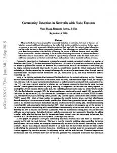
0 whose intercept C is maximized at the point corresponding to the smallest directional component as Theorem 2.2.3 describes. Therefore, the optimization (2.5) leads to the identification of the smaller of the two directional components in this network. To summarize the result, both Proposition 2.2.2 and the example show that the directional components, if there is any, can be identified sequentially by the L0 regularized SVD approach. Recall that we encountered the problem that the small number of external edges connect separate directional communities together as a large directional component. The root of the problem is the strict requirement on finding exact directional components, the maximal set of node satisfying D-connectivity. The L0 regularized SVD limits the number of non-zero entries of the singular vectors, so it may find a community that is embedded and almost separated from the other communities as we have argued in Section 2.2.1. To illustrate the advantage of the regularized approach, we add three external edges in the example. As a result, those two directional components merge together as one, as shown in the left panel of Figure 2.4b. The right panel of Figure 2.4b plots paired values (SZ! ,
1)
of the same 500 pairs of (S, T ) shown
in Figure 2.4a. The principal singular values of the two true directional components 45
y
3 4 5 6 7 8 9 10
1
2
3
4
5
6
7
8
9
x
1
x
0.8
0.6
0.4
0.2
0
10
0
2
4
Adjacency matrix
6
8
10
12
14
16
18
20
22
1
Size of sub-matrix
0.6
0.4
0.2
0
2
4
6
2
x
1
x
3 0.8 4
5 0.6
6 7
0.4
8
0.2
y
y = x+C
9
y = x+C
x 13
1.2
1
Principal singular value
Principal singular value
1.2
1
x
x 0.8
0.6
0.4
0.2
10 0
0
21
42
6 3
48
510
6 12
7 14
8 16 9
18 10
20
22
0
x
Size of sub-matrix Adjacency matrix
0
2
4
6
8
10
12
14
16
18
20
22
x
Size of sub-matrix
(b) After adding three external edges
Figure 2.4: Left panel of (a): The adjacency matrix of an example network having two directional components. Right panel of (a): The scatter plot of SZ! (C(S, T )) and 1 (Q(C(S, T ))). Q(C(S, T )) is a sub-matrix of the graph Laplacian matrix Q derived from the example directed graph. Left panel of (b): The adjacency matrix of the example network of Figure 2.4a after adding three external edges. Right panel of (b): The scatter plot of SZ! (C(S, T )) and 1 (Q(C(S, T ))). Q(C(S, T )) is a submatrix of the graph Laplacian matrix Q derived from the directed graph perturbed by the external edges.
(X marks) have decreased because of the added external edges, but the line with the
46
8
10
12
14
16
Size of sub-matrix
(a) No external edges y
x
x 0.8
0
x
y
x 13
1.2
Principal singular value
Principal singular value
2
y
y = x+C
1.2
1
18
same slope ⌘ is still capable of identifying the original directional component since it still has a low directional conductance value. We have discussed the properties of the directional community obtained by the L0 regularized SVD formulation. Next, we show that it can be solved efficiently through iterative matrix-vector multiplications combined with hard-thresholding of the singular vectors. L0 Regularized SVD Algorithm A local solution of (2.5) can be obtained by the iterative hard-thresholding which is similar to the approach of Shen and Huang (2008) and d’Aspremont et al. (2008). We start with exploiting the bi-linearity of the optimization problem (2.5). For a fixed vector v, we show how to solve the maximization problem with respect to u. Here we first introduce some notations. Given a vector z = (z1 , . . . , zn )0 2 Rn , |z|(l) denotes the l-th largest absolute value of z. Consequently, we define zhl (2 Rn ) as the vector acquired from the hard thresholding of z by its (l + 1)-th largest absolute entry, i.e. the i-th element of zhl is zhl (i) = zi I(|zi | > |z|(l+1) ) while the superscript “h” stands for the hard-thresholding. For a fixed v, we may treat Qv as a generic vector z and find the solution u that maximizes (2.5) through the following proposition. Proposition 2.2.4. For a given vector z and a fixed constant ⇢ > 0, the solution of max ut z
kuk2 1
⇢kuk0
is u = zhl /kzhl k2 , 47
(2.11)
where the integer l is the minimum number that satisfies |z|(l+1)
q ⇢2 + 2 ⇢ kzhl k2 .
(2.12)
When the absolute values of z contains tied values, we pick one arbitrarily. Proof. For a fixed number of non-zero entries kuk0 = l, maxkuk2 1 ut z is obtained when u = zhl /kzhl k2 . Thus the objective function (2.11) can be written as F (l) = kzhl k2
⇢ l.
Now we maximize F (l) over l. Notice that kzhl k2 increases monotonically as l increases. The value of F (l) keeps increasing until q kzhl k22 + |z|2(l+1)
kzhl k2 ⇢,
which is equivalent to (2.12). After l goes beyond this point, F (l) starts to decrease and keeps decreasing because |z|2(l) decreases and kzhl k2 increases. Therefore, the solution to (2.11) is obtained at the minimum l that satisfies (2.12). Proposition 2.2.4 suggests a computationally efficient algorithm to determine the threshold level. We first sort the entries of z by their absolute values and then sequentially search from the largest to smallest while testing if condition (2.12) has been met at each entry. As soon as (2.12) is satisfied, we obtain the hard-threshold level. The computational complexity of this direct-searching algorithm is O(n log(n)). Consequently, the solution of the regularized SVD problem (2.5) is obtained by the searching algorithm for a fixed v and for a fixed u alternatively. Each step increases the objective function monotonically, thus it converges to a local optimal. Algorithm 3 lists the details. 48
Algorithm 3 L0 regularized SVD Require: Q, ⌘, ! 1: initialize v 2: repeat 3: z Qv , ⇢ ⌘ p h h 4: u zl /kzl k2 , where l is the minimum integer s.t. |z|(l+1) ⇢2 + 2 ⇢ kzhl k2 5: z Qt u , ⇢ ⌘! p 6: v zhl /kzhl k2 , , where l is the minimum integer s.t. |z|(l+1) ⇢2 + 2 ⇢ kzhl k2 7: until u, v converged 8: return u, v
The algorithm shows a similarity to HITS algorithm of Kleinberg (1999), but there is a di↵erence as algorithm 3 uses the Laplacian matrix Q instead of the adjacency matrix W . Besides, the algorithm also has the additional step that thresholds the membership vectors. Consequentially, the algorithm can detect a pair of sets of nodes constituting a local community instead it converges to a principal singular vector of Q. This algorithm may not converge to the global solution depending on the initialization. This difficulty stems from the original optimization problem (2.7), which is non-convex and may have local solutions as many as the number of communities. However, the local solutions are in fact reasonable communities we search for because a local solution implies that the community has the lowest conductance among other similar-sized communities nearby.
2.2.3
Regularized SVD with Elastic-net Penalty
In Section 2.2.1, we showed that the L0 regularized SVD may detect tight communities in directed networks and it can be solved by an efficient algorithm based on the power method combined with the hard-thresholding. When the number of 49
external edges is relatively small, we found the L0 regularized SVD performs well. However, when external edges introduce huge perturbation to the spectrum of Q, it may be difficult for (2.5) to identify the communities, for example, in the right panel of Figure 2.4b, the line y = ⌘x + C may hit other o’s before touching the second X. We may consider a slight modification of (2.5) in the following form: max ut Qv u,v
subject to
kuk0 + !kvk0 ,
kuk2 1,
kvk2 1.
(2.13)
It searches for a sub-matrix of Q that has the largest singular value with a strict constraint on its size. The yellow vertical line on the right panel of Figure 2.4b shows the constraint when
= 13. In this case, the solution of (2.13) corresponds to the
second directional component. Although the new formulation provides another option for recovering the directional communities, finding a solution of (2.13) is challenging due to the discrete nature of the constraint. A typical approach to overcome the computational difficulty related to the nonconvexity of the L0 constraint is to relax L0 penalty to L1 penalty. Replacing L0 penalty by L1 penalty and separating the penalty for u and v, we obtain a modified optimization problem, max ut Qv u,v
subject to
kuk1 C1 , kvk1 C2 ,
kuk2 1, kvk2 1.
(2.14)
This optimization problem is identical to a version of the sparse matrix decomposition method proposed in Witten et al. (2009), in which the authors provided an algorithm to find a local solution. The algorithm uses the power method for SVD combined with the soft-thresholding on singular vectors, which has been used in Shen and Huang (2008); Witten et al. (2009); Lee et al. (2010). However we found that the solution of (2.14) did not report significantly better solutions than L0 regularized SVD solution 50
from (2.5) in our simulation studies. One possible reason is that L1 constraint may fail to give sufficiently sparse solution of u and v, as pointed out by Yang et al. (2011). As an alternative, we propose a regularized SVD with the Elastic-net type penalty (Zou and Hastie 2005), max ut Qv,
(2.15)
u,v
subject to
(1
↵)kuk22 + ↵kuk1 c1 ,
(1
)kvk22 + kvk1 c2 ,
where the sparsity level is controlled by the parameters ↵ 2 [0, 1) and that ↵ =
= 0 leads to the regular SVD problem. When ↵ 2 (0, 1) and
2 [0, 1). Note 2 (0, 1), the
optimization problem becomes non-convex. We show that a local solution of (2.15) can be found by the power method with the soft-thresholding. Elastic-net Regularized SVD Algorithm Similar to the calculation of the L0 regularized SVD, we take advantage of the bi-linearity of the optimization problem. For fixed v and ↵, (or u and ), the optimization becomes convex, max ut Qv, u,v
subject to
↵)kuk22 + ↵kuk1 c1 ,
(1
(2.16)
whose global solution can be obtained through a soft-thresholding. We note that Witten et al. (2009) and Lee et al. (2010) showed similar results under slightly di↵erent constraints. To find the solution of (2.16), we first introduce a definition: Definition 2.2.5. For a vector z = (z1 , . . . , zn )0 2 Rn , recall the l-th largest absolute value of z was defined as |z|(l) . Denoting |z|(n+1) = 0 for convenience and we define k(x) 1 1 X Gz (x) = 2 (|z|(i) 4x i=1
k(x) 1 1 X x) + (|z|(i) 2x i=1 2
where k(x) 2 {1, . . . , n + 1} satisfies |z|(k(x)) x < |z|(k(x) 51
1) .
x)
(2.17)
From Witten et al. (2009) we borrow a notation, S(z, d), as the result of softthresholding a vector z by a scalar d. Soft-thresholding is defined by S(z, d) = sign(z)(|z|
d)+ , where d > 0 and x+ = max{x, 0}. Again treating Qv as a generic
vector z, we find the solution u that maximizes (2.16) by the following theorem: Theorem 2.2.6. For a fixed vector z, the solution of the optimization problem, max u
ut z,
subject to (1
↵)kuk22 + ↵kuk1 c1
is u=
2d(1 ↵) S(z, d), ↵
and the threshold level d is the solution of Gz (d) = c1 (1
↵)/↵2 .
The proof of the theorem is provided in the Appendix A.4 and its first part resembles the proof of Lemma 2.2 of Witten et al. (2009). This theorem leads to Algorithm 4. The computation in Algorithm 4 involves solving for the soft-threshold level d in the equation Gz (d) = c, where c is some constant in the range of the function Gz (·). The way to determine the threshold level d is described in Lemma 2.2.7.
Algorithm 4 SVD with elastic-net penalty Require: Q, ↵, , c1 , c2 1: initialize v 2: repeat 3: d the solution x of GQv (x) = c1 (1 ↵)/↵2 2d(1 ↵) 4: u S(Qv, d) ↵ 5: d the solution x of GQt u (x) = c2 (1 )/ 2 2d(1 ) 6: v S(Qt u, d) 7: until u, v are converged 8: return u, v
52
Lemma 2.2.7. The solution of the equation Gz (d) = c for given c > 0 is 0 Pˆ 1 12 k 2 i=1 |z|(i) A , d=@ 4c + kˆ
(2.18)
where kˆ is a positive integer in {1, 2, . . . , n} that satisfies Gz (|z|(k) )> ˆ ) c, Gz (|z|(k+1) ˆ c. Proof. For the first step, we show that Gz (·) is a monotone decreasing function, that is, if d1 > d2 , then Gz (d1 ) < Gz (d2 ). The first term of (2.17) is monotone decreasing of d because k(d2 ) 1 1 X (|z|(i) 4d22 i=1
k(d1 ) 1 1 X d2 ) > 2 (|z|(i) 4d1 i=1 2
k(d1 ) 1 1 X > 2 (|z|(i) 4d1 i=1
d2 )2 d1 )2 .
The first inequality comes from the fact that k(d2 ) k(d1 ) and d1 > d2 . The second inequality comes from d1 > d2 . The second term of (2.17) can be done in the similar way and the desired result is obtained. For the second step, we find an approximated solution of d from the set of {|z|(i) }i=1...n . By plugging in |z|(i) to d in the increasing order of i, we can find kˆ such that Gz (|z|(k) ) > c by the monotonicity of Gz (·) and being c in ˆ ) c, Gz (|z|(k+1) ˆ the range of Gz (·). This computation can be done efficiently by computing two cuP P mulative sums, ki |z|2(i) and ki |z|(i) , in the increasing order of k until kˆ is obtained. The algorithm for finding kˆ in this Lemma is provided in Algorithm 5.
From the second step, we already know that |z|(k+1) < d |z|(k) ˆ ˆ which means k = kˆ fixed now. Therefore solving a quadratic equation of d, ˆ k 1 X (|z|(i) 4d2 i=1
ˆ k
1 X d) + (|z|(i) 2d i=1 2
53
d) = c,
Algorithm 5 Find kˆ such that Gz (|z|(k) )>c ˆ ) c, Gz (|z|(k+1) ˆ Require: (z1 z2 , . . . , zn ), c > 0 1: initialize S1 0, S2 0, kˆ 2 2: for k = 2 : n do 3: S1 S1 + z k 1 4: S2 S2 + zk2 1 5: Gk = 4z12 (S2 2zk S1 + (k 1)zk2 ) + k 6: if Gk > c then 7: kˆ k 1 8: return kˆ 9: end if 10: end for 11: if Gk c then 12: kˆ n 13: return kˆ 14: end if
1 (S1 2zk
(k
1)zk )
determines the solution d. By the quadratic formula, the solution is 0 Pˆ
knowing that d > 0.
d=@
k i=1
|z|2(i)
4c + kˆ
1 12
A ,
Our contribution is that we seek the threshold level d in nearly linear time that is proportional to the number of non-zero entries of the solutions, which makes the computation feasible for large matrices in comparison to the binary search method proposed in Witten et al. (2009). Even though we have assumed Q is a nonnegative matrix, the linear search method can be applied to any real valued matrix. In fact, (2.14) can also be solved using the linear search method instead of the binary search method. We have empirically confirmed that the linear search method is faster than the binary search method by 3 to 20 times when the number of nodes in the network is between 103 and 107 . 54
In summary, we proposed two linearly scalable algorithms, the L0 regularized SVD and the Elastic-net regularized SVD, for extracting one community from a directed network. In the next section, we propose a general method that extracts directional communities sequentially by applying the community extraction algorithm repeatedly to a network.
2.2.4
Community Extraction Algorithm
We first emphasize the computational advantage of identifying one community at a time for large networks. For example, Clauset (2005) discussed an approach of local community detection in the application of World-Wide-Web, which cannot even be loaded to a single machine’s memory. Algorithm 3 uses only the out-links of the current source nodes and the in-links of the current terminal nodes in the matrix multiplication steps. We will exploit this property to devise a local community detection algorithm. The regularized SVD algorithms require the sparsity parameters, ⌘ in (2.5) or (↵, ) in (2.15) and a starting vector v or u to initialize the algorithm. In this section, we first discuss the e↵ect of these parameters and how to choose them in practice. Then we propose a community harvesting scheme that repeatedly use the regularized SVD algorithm to extract multiple communities. Parameter Selection and Initialization for Regularized SVDs We now study the e↵ect of the penalization parameters on the algorithm outputs. First, for Elastic-net regularized SVD, we point out that the parameters c1 and c2 in (2.16) can be set to one as default, since they only a↵ect the magnitude of the solution vectors. Second, we find that imposing di↵erent sparsities to source nodes 55
and terminal nodes can be a useful modification to the algorithms. However, we leave the investigation as a future work and we assume the same sparsity levels in the rest of this paper. Thus, we set w = 1 for the L0 regularized SVD and ↵ =
for the
Elastic-net regularized SVD. We propose to use the directional conductance (C(S, T )), which is presented in (2.3), to find the best community among candidate communities. Computing
is
inexpensive even for a large network if degrees of nodes and the number of edges are already computed. Although
may not be an ideal measure for comparing
communities in considerably di↵erent sizes, it is still a decent measure for similarsized communities. Thus, we will look for the community achieving a local minimum value of
over the smooth change of the candidate communities.
The candidate communities are obtained by changing sparsity parameters (⌘ for L0 regularized SVD, ↵ for EN regularized SVD) smoothly. The solution v⇤ at the current sparsity level is taken as the initial vector at the next contiguous sparsity level. The small changes in the sparsity level make the algorithm converge in several iterations without causing dramatic alterations in the solution at the new sparsity level. Furthermore, we start the searching with a large sparsity level, so that the algorithms investigate relatively small sub-networks in the initial stages. As a result, provided a sequence of decreasing sparsity levels, we obtain a sequence of growing candidate communities and select the best one regarding the directional conductance. We name the identified community (S, T ) from this method a Approximated Directional Component (ADC), to distinguish it from the directional components. The procedure is described in Algorithm 6. We note that one may simply replace the L0
56
Algorithm 6 Community Extraction via L0 Regularized SVD Require: Q, initialization vector v0 , decreasing sequence of sparsity levels {⌘i }i=1,...,I 1: initialize v v0 2: for i = 1 to I do 3: Obtain u⇤ , v⇤ by running Algorithm 3 with (Q, ⌘i ) and initialization v. 4: S = {v : u⇤ (v) 6= 0} and T = {v : v⇤ (v) 6= 0} 5: (C(S, T )) i 6: (S i , T i ) (S, T ), v v⇤ 7: end for 8: return S = S j and T = T j , where j corresponds to a local minimum in { 1 , . . . , I }.
regularized SVD with Elastic-net regularized SVD to attain another version of the algorithm. The algorithm requires a user to specify the initialization vector v0 and the sequence of the sparsity level parameters. The initialization vector v0 can be set as 1{vi } with a randomly picked vi with nonzero degree or can be set as the node with a large degree to discover the larger communities first. We use the later as default in what follows. The searching for candidate communities can be stopped early if the conductance value reaches a local minimum of a sufficiently low directional conductance. A simple implementation is to stop searching if the conductance value of the current candidateADC bounces up to higher than sp (sp > 1) times of the minimum conductance value of the previously detected candidate-ADCs. Besides, we pre-specify a bound sl (0 < sl < 1) on the desired conductance value so we only stop searching early at a candidate-ADC with the conductance value lower than sl . This stopping rule saves computation burden and keeps the quality of communities. We will use this early stopping rule in Section 2.3. 57
Spar s ity = 0.60
Spar s ity = 0.40
0
0
10
10
20
20
30
30
40
40
50
50
60 0
20
40
60 0
60
Spar s ity = 0.15 0
10
10
20
20
30
30
40
40
50
50
20
40
40
60
Spar s ity = 0.10
0
60 0
20
60 0
60
20
40
60
Figure 2.5: A simulated directed graph from stochastic block model. The probability of existing edges is 0.3 for within a community and 0.05 for between communities. There are 20 source nodes and 20 terminal nodes for each directional community. A community structure is revealed at the sparsity level 0.15.
We present an example that shows snap-shots of the solutions corresponding to several di↵erent sparsity levels. A network of size 60 with 3 directional communities is simulated from the stochastic block model (Holland et al. 1983). For the three communities, the probability of a directed edge existed between any ordered pair of nodes, (vs , vt ), is set to 0.3 if the edge is within a community and the probability is set to 0.05 otherwise. A realization of the network is shown in the form of the adjacency matrix in Figure 2.5. We observe three strong blocks of dense connections.
58
A solution path from the Elastic-net regularized SVD is obtained with an initialization vector v = 1{v1 } and parameters ↵ decreasing from 0.8 to 0.1 by a step size of 0.05. The panels in Figure 2.5 show the extracted communities (in red dots) at four di↵erent sparsity levels ↵ = 0.6, 0.4, 0.15, 0.1 on the path. As we expected, it is obvious to observe the nested structures among the detected communities on the solution path. The algorithm captures the most links in a directional community at the sparsity level 0.15 while not including too many external edges. The conductance values of the four di↵erent results shown in Figure 2.5 are 0.621, 0.521, 0.373 and 0.412, which correspond to the penalization parameter at 0.6, 0.4, 0.15, and 0.1, respectively. The minimum conductance value over the detected communities is 0.373, which leads us to pick the results at the sparsity level ↵ = 0.15. Another interesting observation in this example is the dependence between the extracted community and the initial vector. Since both the regularized SVD algorithms are based on the local updatings, their outputs are sensitive to the initial vector v0 . In the example, the algorithm would have recovered another collection of links on the other community if it had started from v0 = 1{v30 } . Community Harvesting Algorithms In order to identify all tight communities in a directed network, we propose to apply Algorithm 6 repeatedly through a community harvesting scheme. The idea of community extraction has been discussed in Zhao et al. (2011), in which a modularity based method is introduced. Starting with the graph Laplacian matrix Q of the full network, we first apply Algorithm 6 with L0 or Elastic-net penalty to identify an ADC(S, T ). Then the entries of Q that correspond to the weight of edges in the identified ADC(S, T ) are 59
set to zero and we reapply the algorithm again to the reduced Q matrix with a di↵erent initialization in order to identify the next ADC. It continues until the remaining edges are less than a pre-determined number M , to say 10% of the original number of edges. Typically, the remaining network contains only tiny directional components which are mainly originated from the edges between communities. We call this procedure community harvesting algorithm, which is presented in Algorithm 7.
Algorithm 7 Community Harvesting Algorithm Require: Q, i = 1, M 1: repeat 2: Obtain S, T using Algorithm 6 with Q and 1{vi } (vi is a positive degree node of Q) 3: Nullify the identified sub-matrix, Q(C(S, T )) 0 4: Si S, Ti T 5: i i+1 6: until Q has lower than M non-zero entries 7: return {ADC(Sj , Tj )}j=1,...,i
The harvesting algorithm takes a di↵erent approach from the other sparse SVD algorithms devised for obtaining multiple sparse singular vectors. Witten et al. (2009) and Lee et al. (2010) use the residual matrix, Q
suvt where s is pseudo singular
value, to obtain the multiple sparse singular vectors. This approach does not fit to our purpose since only the principal singular vector of a submatrix is required for a directional component. In addition, harvesting algorithms get Q more sparse as ADCs are harvested along the way whereas the other approaches have to deal with the residual matrices which are more dense than the original adjacency matrix. For a massive network, a dense matrix is simply not a↵ordable computationally.
60
The scheme of harvesting edges of a detected community also allows multiple memberships for the nodes in both of source parts and terminal parts. On the other hand, this sequential removal of edges may give a concern regarding the stability of the detected communities. We observed the communities with the low directional conductance ( ) are stable under the di↵erent initializations and the order of extractions. Depending on the situation and purpose, one may consider harvesting nodes instead of harvesting edges. Of course, if one has a strong prior knowledge that a node has a single membership of a community, harvesting nodes would be appropriate. On the other hand, harvesting edges provide more flexibility in the community structure as it allows multiple memberships. We observed that harvesting nodes does not give significantly di↵erent outcomes if a network has strong communities.
2.2.5
Computational Complexity of Harvesting Algorithms
A driving motivation of the harvesting algorithm is the scalability on massive networks. Here, we investigate the harvesting algorithms’ computational complexity and computer memory requirements. In the specification of harvesting algorithms discussed in Section 2.2.4, there are four parameters that mainly determine the computation time: the number of sparsity levels (I), the number of detected communities (K), the number of edges (m), and the number of nodes (n). The complexity of a harvesting algorithm is O(IK(m+n log n)). If the optimal sparsity level is known, I can be dropped. Parallel computing may potentially reduce the computation time by the factor of K if multiple communities can be searched simultaneously.
61
The computer memory requirement is mainly determined by m. But for a huge network that cannot be fit into a machine, relatively small sub-network can be exP plored locally. The regularized SVDs only require a sub-network of vi 2S dr,i + P vi 2T dc,i edges and the source part S and the terminal part T change smoothly over the iterations. We leave a parallel version of the harvesting algorithm for a future research, which is a promising approach to tackle massive modern networks. The computational time may vary depending on the settings of the algorithm, the software implementation and the data at hand. We report the actual computation times for the two large networks, a citation network and a social network, in Section 2.3.
2.2.6
Simulation Study
In this section, we evaluate the performance of the two harvesting algorithms, L0 harvesting and EN -harvesting under the various settings of community structures. In addition to the harvesting algorithms, DI-SIM algorithm is included for the sake of comparison. We find that, in addition to the proportion of external edges, the average degree and the size of communities are also important factors determining the accuracy of community detection methods. Benchmark Model To generate networks with di↵erent types of community structures, we follow a benchmark model proposed by Lancichinetti et al. (2008), referred as the LFR model. The LFR model is based on a restricted version of the stochastic block model where each node has a probability of being connected to nodes in the same community and another probability of being connected to nodes in other communities. This 62
benchmark model is originally developed for undirected networks but it has been extended to directed networks by Lancichinetti and Fortunato (2009b). The LFR model introduces heterogeneous degrees of nodes and community sizes. The outdegrees of all nodes are almost constant while the in-degrees follow a power law distribution introduced in (1.1). This model is more suitable than GN benchmark of Girvan and Newman (2002) in asymmetric networks such as citation networks and online social networks. As a remark, currently LFR model only generates symmetric directional communities, which means the source part and the terminal part consist of the same nodes. Harvesting algorithms are capable of detecting directional communities regardless of their symmetricity while the most existing algorithms are only capable of detecting highly symmetric communities. For example, in asymmetric communities, we have tested the performance of Infomap algorithm for directed networks, which is reported being the best algorithm in detecting symmetric communities in the LFR model (Lancichinetti and Fortunato 2009a). To generate a network with asymmetric communities, the labels of terminal nodes of the network generated by the LFR model are shu✏ed. The Infomap algorithm could not detect the asymmetric community structure, only providing a single community, which is the whole network. In the simulation study, we generate networks from the LFR model with n = 1000 nodes, whose in-degrees follow a power law (with decay rate ⌧1 =
2) with maximum
at kmax = 50. The sizes of the communities in each network are assumed to follow a power law with a decay rate ⌧2 =
1 and the sizes of source part and terminal part
are the same. We vary three sets of parameters of LFR model to control di↵erent aspects of the simulated networks: 63
• Range of community sizes is set at two levels through a pair of parameters (SZ!=1 (C)min , SZ!=1 (C)max ): (40, 200) for big communities and (20, 100) for small communities; • Average degrees (in-degree and out-degree) k for all nodes are set at three levels: {5, 10, 20} for sparse, median and dense networks; • Proportion of external edges µ for all nodes is set at three levels: {0.05, 0.2, 0.4}.
Original
0 200
200
300
300
600
600
800
800
1000 0
200
400
600
800
1000 0
1000
L0 -harvesting
0
0
200
200
300
300
600
600
800
800
1000 0
200
400
600
DI-SIM
0
800
1000 0
1000
200
400
600
800
1000
EN -harvesting
200
400
600
800
1000
Figure 2.6: A random matrix generated by LFR benchmark and the results of DI-SIM algorithm and harvesting algorithms (top right: DI-SIM, bottom left: L0 -harvesting, bottom right EN -harvesting).
Before providing the details of simulation results, we show an example of the simulated network and the results of the three community detection methods in Figure 2.6. 64
This network with big communities, (SZ!=1 (C)min , SZ!=1 (C)max ) = (40, 200), is generated with parameters k = 20 and µ = 0.1. Rows of matrix correspond to source nodes and columns correspond to terminal nodes while each dot in the plot represents an edge. The top left panel is the adjacency matrix of the simulated network. The rest of panels present community structures found by the three algorithms in comparison. By the design of the DI-SIM algorithm, it provides two unrelated partitions for rows and columns. In contrast, the harvesting algorithms recover directional communities by collecting edges of each community and they indeed showed almost perfect recovery in this example. Simulation Study with LFR Benchmark Back to the full simulation, the accuracy of community detection results is measured by a mutual information based criterion that was proposed by Lancichinetti et al. (2009). The criterion is used for the comparison of various community detection algorithms by Lancichinetti and Fortunato (2009a). One advantage of this criterion is its ability to handle overlapping communities, see details in the appendix of Lancichinetti et al. (2009). Like other mutual information based criteria, the accuracy measure has the maximum value one for the perfect match and has the minimum value zero for the community assignment that is independent of the true community structure. The accuracy of the algorithms were computed by comparing the discovered communities {Ci (S, T )}i=1,...,k to the true directional communities. When applying the DI-SIM algorithm, we assume the true number of communities NC is known. We compute the first NC singular vectors of Q and apply the kmeans algorithm with NC clusters on the left and right singular vectors separately. One hundred random initialization for the k-means algorithm is applied and the one 65
minimizing the within-cluster sums of point-to-cluster-centroid distances is taken as the final outcome. DI-SIM algorithm does not produce directional communities, since it results in two di↵erent partitions, a partition for source nodes and a partition for terminal nodes. As an ad-hoc, we match the source part and the terminal part by the largest common edges. Harvesting algorithms are initialized with v0 being the node of largest in-degree at each harvesting. The sparsity levels for the source part and the terminal part are set to the same value, ! = 1 in (2.5) and ↵ =
in (2.15). The sequence of them are
determined so that the detected communities are sized roughly SZ!=1 (C) 2 (20, 400). More specifically, the grid of sparsity levels for L0 penalty, ⌘, contains 10 points in {exp( k) : k = 6 + i(5/10), i = 1, . . . , 10} and the grid of sparsity levels for EN 1 penalty, ↵, includes 10 points in { 1+exp(k) : k = 1 + i(3.7/10), i = 1, . . . , 10}. Those
non-linear grids are adapted to obtain more constant changes in the size of candidate communities. Early stopping parameters are set to sp = 1.5 and sl = 0.6. The harvesting algorithm continues until the number of harvested communities reaches the true number of communities or there is no more edges left. In this simulation, we generate 30 random networks under each of the eighteen (2⇥ 3⇥3) parameter combinations and the average accuracy of each algorithm is reported. The results for networks with large communities and those with small communities are reported in Figure 2.7 and Figure 2.8 respectively. In these figures, each of the nine panels on the left side visualizes a sample of the generated networks for each simulation setting, and the box-plots on the right side show the corresponding accuracy of the four di↵erent algorithms. Recall that the range of the accuracy measure is [0, 1] and the larger the value, the better the accuracy. Here, the accuracy of Infomap is 66
displayed only for the reference, which is the performance of the state-of-art algorithm in detecting symmetric directional communities. We want to emphasize that the performance of Infomap on asymmetric directional communities is unsatisfactory and not even comparable to the accuracy of the other algorithms which are capable of detecting asymmetric communities. The results for the big communities in Figure 2.7 show that the harvesting algorithms report almost perfect recovery when nodes have average degree of 10 and µ = 0.05, 0.2, and average degree of 20 and µ = 0.05, 0.2, 0.4. The networks with such average degree and µ correspond to the strong community structure that ensures D-connectivity of the members in true directional components and relatively small fraction of external edges. The EN -harvesting shows better performance than the L0 -harvesting in the region of strong community structure. Moreover, the EN harvesting gives almost perfect recovery in the setting of µ = 0.4 and average degree 20. As we have mentioned in Figure 2.6, the DI-SIM algorithm fails to give a perfect result even for the high average degrees. However, the DI-SIM algorithm gives better results than harvesting algorithms in the region of relatively weak community structures, for example, in the setting of µ = 0.4 and average degree 5. The accuracy of the algorithms for detecting small communities change slightly from the ones for big communities (Figure 2.8). The accuracy of the L0 -harvesting method have decreased in the regions of high degree and low µ. The accuracy of the EN -harvesting algorithm is similar to the result of big communities. However, the k-means algorithm in DI-SIM algorithm seems to be less accurate for the larger number of clusters in the setting of small communities.
67
A closer investigation revealed that the reasons for the loss in accuracy are quite di↵erent for the harvesting algorithms and the DI-SIM algorithm. The loss of accuracy of the DI-SIM algorithm mainly stemmed from some clusters dividing true communities. In contrast, the loss of accuracy of harvesting algorithms mostly came from the several ADCs merging true communities. In such case, those communities can be improved by applying the harvesting algorithm recursively on the merged community. We will further discuss this idea in Section 4.2. In our experiment, we also find that the performance of harvesting algorithms is as good as that of Infomap, which shows the best performance in the report of Lancichinetti and Fortunato (2009a). However, the performance of Infomap grounds on the assumption that the true communities have the same source part and terminal part, i.e. S = T , and the performance can dramatically drop without the assumption. In contrast, harvesting algorithms do not require such assumption on the true communities since the source part and the terminal part of a directional component may be totally di↵erent.
68
Community Detection Accuracy
Networks with Big Communities
|E| = 5608
|E| = 10107
|E| = 19763
|E| = 5889
|E| = 10130
|E| = 19613
|E| = 5524
5
|E| = 10107
10
|E| = 19321
20
Average degree (a) Adjacency matrices of networks with big communities. Rows and columns are arranged by the true communities.
0.75
0.4
0.50 0.25 0.00 1.00
method
0.2
0.75
L_0
0.50
EN DI−SIM
0.25
Infomap
0.00 1.00 0.75
0.05
0.05
0.05
20
0.2
0.2
Proportion of external edges (µ)
0.4
10
0.4
69
Proportion of external edges (µ)
5 1.00
0.50 0.25 0.00
5
10
20
Average degree (b) Community detection accuracy of four tested algorithms, from left L0 -harvesting, EN -harvesting, DI-SIM and Infomap.
Figure 2.7: Accuracy of the four algorithms, L0 -harvesting, EN -harvesting, DI-SIM and Infomap in the nine di↵erent settings of the community structure. The x-axis indicates the average degree and the y-axis indicates the proportion of external edges. The left panel shows an example network at each setting. The accuracy is displayed as bar charts in the right panel. The size of communities ranges in 40 ⇠ 200. The accuracy of Infomap cannot be directly compared to other methods since they are measured in the symmetric directional communities while other three methods are applied on the asymmetric directional communities.
Community Detection Accuracy
Networks with Small Communities
|E| = 5637
|E| = 9871
|E| = 19470
|E| = 5601
|E| = 10154
|E| = 19645
|E| = 6197
5
|E| = 9669
|E| = 19191
10
20
Average degree (a) Adjacency matrices of networks with small communities. Rows and columns are arranged by the true communities.
0.75
0.4
0.50 0.25 0.00 1.00
method
0.2
0.75
L_0
0.50
EN DI−SIM
0.25
Infomap
0.00 1.00 0.75
0.05
0.05
0.05
20
0.2
0.2
Proportion of external edges (µ)
0.4
10
0.4
70
Proportion of external edges (µ)
5 1.00
0.50 0.25 0.00
5
10
20
Average degree (b) Community detection accuracy of the four algorithms, from left L0 -harvesting, EN -harvesting, DI-SIM and Infomap.
Figure 2.8: Accuracy of the four algorithms, L0 -harvesting, EN -harvesting, DI-SIM and Infomap, in the nine di↵erent settings of the community structure. The x-axis indicates the average degree and the y-axis indicates the proportion of external edges. The left panel shows an example network at each setting. The accuracy is displayed as bar charts in the right panel. The size of communities ranges in 20 ⇠ 100. The accuracy of Infomap cannot be directly compared to other methods since they are measured in the symmetric directional communities while other three methods are applied on the asymmetric directional communities.
2.3
Communities in Real Networks
In this section, we apply the proposed harvesting algorithms to highly asymmetric directed networks, a paper citation network and a social network. Paper citation networks are highly asymmetric because of their temporal structure; a paper can cite only existing papers. The social network used in this application is highly asymmetric due to a small fraction of popular users with a high fraction of total in-degrees. We show that the harvesting algorithms can capture the communities reflecting two di↵erent roles of nodes even in such highly asymmetric directed networks.
2.3.1
A Citation Network
We first apply both harvesting algorithms to the Cora citation network, a directed network formed by citations among Computer Science (CS) research papers2 . In this experiment, we use a subset of the papers that have been manually assigned to the categories that represent 10 major fields in computer science, which is further divided into 70 sub-fields. The citations result in a network of 30,228 nodes and 110,654 edges after removing self-edges. In this citation network, only 5.4% of edges are symmetric. The average degree is 3.66, which is relatively low. We also found that 2345 nodes had error labels and they were put into 11th category. The algorithms start at the terminal nodes with the largest in-degree among unharvested nodes at each harvesting run. The sparsity levels are determined so that candidate ADCs may cover up to 50% of nodes. The sparsity parameter ⌘ in the L0 -harvesting takes the decreasing values in a grid {exp( k) : k = 10 + i(8/200), i = 2
http://people.cs.umass.edu/~mccallum/data.html
71
1, . . . , 200}. Similarly, the sparsity parameter ↵ in the EN -harvesting takes the de1 creasing values in a grid { 1+exp(k) : k = 2 + i(7/200), i = 1, . . . , 200}. The nonlinear
decreasing setup is utilized to obtain gradual expansions of the candidate-ADCs at the low sparsity levels. Early stopping parameters are set to sp = 1.4 and sl = 0.4. Each algorithm runs until it harvests 90% of edges. L0 -harvesting discovered 51 communities in 4 minutes and EN -harvesting discovered 78 communities in 9 minutes. For both harvesting algorithms, we first provide a summary of the largest twenty ADCs discovered. The sizes of source part and terminal part, the number of edges and conductance value for each ADC are reported in Table 2.1. We name the ADC obtained in the L0 -harvesting ADC L0 and the ones obtained by the EN -harvesting ADC EN . Out of total 110,654 edges, the first twenty ADC L0 s cover 82,372 edges (74%) and the first twenty ADC EN s cover 88,756 edges (80%). We observe that larger communities are likely to be captured in the first several ADCs because the initial value v0 for each harvesting is correponding to a high in-degree node. Most detected communities have larger source parts than the terminal parts, and it reflects the presence of the late papers that are not yet cited much. Overall, we also found that ADC L0 s are better than ADC EN s based on the comparison of the conductance values. This result is consistent with the simulations in Section 2.2.6 that L0 -harvesting performs better in networks of low average-degrees Comparison to DI-SIM and Infomap The performance of harvesting algorithms is evaluated along with two existing community detection algorithms for comparison. First, the DI-SIM algorithm (Rohe and Yu 2012) is applied, assuming the number of communities are equal to the number of major-fields in CS, which is ten. For the k-means step of the DI-SIM algorithm, the 72
Order 1 2 3 4 5 6 7 8 9 10 11 12 13 14 15 16 17 18 19 20
|S|
3266 2636 1543 1381 1270 803 694 577 573 583 539 503 587 479 390 368 370 334 291 226
|T |
2321 1886 1128 971 919 512 480 485 447 361 368 403 278 251 278 233 207 171 207 154
|E|
Order
21851 0.1500 12972 0.2244 8342 0.1724 4690 0.2034 6037 0.1910 3790 0.1271 4143 0.3638 2299 0.4906 2018 0.3070 2455 0.4363 2522 0.3033 1580 0.3588 1750 0.4666 1659 0.2909 1558 0.3031 938 0.4609 1007 0.3271 970 0.2416 1119 0.2312 672 0.4978
1 2 3 4 5 6 7 8 9 10 11 12 13 14 15 16 17 18 19 20
(a) First 20 ADC L0 .
|S|
5319 4458 2309 2254 914 752 643 528 441 453 258 225 245 195 187 187 191 162 141 168
|T |
3176 2756 1535 1546 650 488 444 323 304 276 139 164 116 130 136 132 120 94 115 80
|E|
25428 17137 10422 14539 3127 3219 2522 1561 1487 1602 1504 987 1515 558 555 629 512 512 510 430
0.2579 0.2437 0.2626 0.2176 0.3839 0.3605 0.4176 0.3223 0.3702 0.2505 0.2965 0.3794 0.2070 0.3265 0.5642 0.2128 0.3706 0.2834 0.4501 0.2624
(b) First 20 ADC EN .
Table 2.1: Summary of the largest 20 ADCs of Cora citation network.
best clustering is selected among the outcomes of ten random initializations. Second, we applied the Infomap algorithm of Rosvall et al. (2009), which showed excellent performance in the LFR benchmark as well reported by Lancichinetti and Fortunato (2009a). To show overall di↵erences, we present a visual comparison of communities detected by these four algorithms in Figure 2.9. The visualization of the results of harvesting algorithms through the adjacency matrix is not straightforward since the nodes may appear more than once due to the possibility of multiple memberships. To 73
(b) EN -harvesting
(a) L0 -harvesting 4
0
x 10
0.5 1 1.5 2 2.5 3 0
1
2
3 4 x 10
(d) Infomap
(c) DI-SIM
Figure 2.9: Top panels (a,b): The results of harvesting algorithms on the Cora citation network. The rows and columns are arranged by the source parts and the terminal parts of the first twenty ADCs and remaining nodes are appended at the end of rows and columns. Bottom panels (c,d): Adjacency matrix of the Cora citation network with rows and columns reordered by the results of the DI-SIM algorithm and Infomap.
74
see the community structure, the rows and columns are arranged by the source parts and the terminal parts of the twenty approximated directional components and the remaining nodes are appended at the end of rows and columns. Edges are shown as blue dots in the plot. Internal edges of ADC appear as blue blocks in the diagonal and all internal edges appear only once in the visualization. Meanwhile, blue dots outside the blocks are the edges that are not harvested in the first twenty harvesting. As the harvesting goes on, all edges outside the blocks will eventually append to the diagonal blocks and appear as a thin line at the end of the diagonal. We also use yellow dots to indicate the reappearing internal edges of ADCs that appear between blocks because of the multiple memberships of source nodes and terminal nodes. The lower panels in Figure 2.9 show the results of the existing methods. The result or the DI-SIM algorithm is summarized by the adjacency matrix of the Cora citation network with rows and columns reordered by the partitions (Figure 2.9c). The row of matrix is reordered by the partition of the source nodes and the column of matrix is reordered by the partition of the terminal nodes. The adjacency matrix rearranged by the communities of Infomap is shown in Figure 2.9d, in which the order of rows and columns are the same as the detected communities are symmetric. Comparing all four panels, we conclude that the obvious block structure in the plots of L0 -harvesting better represents the community structure in the Cora citation network. The communities detected by the harvesting algorithms reveal distinct representation of the underlying structure. First, harvesting algorithms capture the asymmetric nature of communities in the citation network. The symmetric assumption of Infomap
75
yields tiny communities that are less significant. Second, the proposed algorithms reveal correspondence between source nodes and terminal nodes while DI-SIM treats them separately. Correspondence between Communities and Manual Categories The manually assigned categories of papers (Table 2.2) in the Cora citation network provided us with extra information to validate the quality of detected communities. The sizes of di↵erent categories span a large range, from 582 papers in Information Retrieval to 10,784 papers in Artificial Intelligence. Given the categories, we calculate the conductance value of each category to see the quality of a category as a community. Those values are overall greater than those of ADC L0 s presented in Table 2.1.
Number 1 2 3 4 5 6 7 8 9 10
Name of Major Field of CS
Number of Papers
Artificial Intelligence Data Structures Algorithms and Theory Databases Encryption and Compression Hardware and Architecture Human Computer Interaction Information Retrieval Networking Operating Systems Programming
10784 3104 1261 1181 1207 1651 582 1561 2580 3972
0.1568 0.3854 0.3429 0.4096 0.4762 0.4527 0.3932 0.3686 0.3736 0.3178
Table 2.2: List of ten fields of Computer Science and their number of papers and conductance.
We investigate the consistency between the detected communities of each algorithm and the manually assigned categories. The communities of L0 -harvesting algorithm are reported in detail in Table 2.3, while the results of other algorithms can 76
be found in Appendix A.5. The communities are reported by their order of being harvested.
1 2 3 4 5 6 7 8 9 10 11 12 13 14 15 16 17 18 19 20
AI
DSAT
DB
106 2741 13 727 284 149 16 40 283 18 651 524 543 492 427 104 21 20 243 292
199 68 12 124 83 452 40 90 184 38 1 7 23 4 11 6 9 66 14 1
56 30 25 8 803 3 95 14 0 30 0 3 1 10 0 23 3 2 0 1
EC
HA
HCI
IR
Net
OS
Prog
Uncategorized
18 255 9 8 115 11 102 12 9 9 239 12 19 94 14 32 8 29 13 2 2 1 1 0 3 2 8 8 8 0 3 3 307 3 0 221 7 15 3 0
17 28 307 577 17 0 32 11 19 28 1 22 1 2 1 187 8 0 1 5
0 63 18 10 66 2 7 0 1 0 24 73 45 1 3 12 2 0 0 7
55 17 936 6 14 3 50 112 3 27 0 1 0 0 0 0 20 26 1 0
900 34 232 22 16 9 347 254 32 355 0 2 9 0 3 13 40 6 12 0
1779 75 34 21 80 6 96 157 37 127 4 22 31 3 3 110 22 15 34 0
467 223 167 123 154 63 105 125 135 102 29 45 54 35 34 49 22 33 39 24
Table 2.3: Number of papers in the first twenty approximated directional components of L0 -harvesting for each category.
The first six harvested communities are fairy large and reveal interactions among the fields of CS. Papers in ADC1L0 are mainly coming from two fields, operating system (OS) and Programming (Prog). ADC2L0 mainly consists of the papers from artificial intelligence (AI), more specifically, the machine learning sub-field. ADC3L0 includes majority (60%) of papers in networking (Net). ADC4L0 are dominated by papers from
77
AI and human computer interaction (HCI) and further investigation showed that the majority of these papers in AI are in the vision and pattern recognition sub-field, which is closely related to HCI. ADC5L0 also contains majority (64%) of papers in databases. ADC6L0 indicates the interplay between data structures algorithms and theory (DSAT) and Encryption and compression (EC). The rest of those communities are smaller in sizes and each contains less diverse categories. In other words, the small communities have high precision and low recall with respect to the manual categories. Many of the small communities are related to L0 the AI category and they represent di↵erent sub-fields of AI. For example, ADC11 L0 corresponds to speech sub-field and natural language processing sub-field. ADC12
mainly covers knowledge representation sub-field. There are also meaningful small L0 communities from the fields other than AI, for instance, ADC18 stands for logic
design and VLSI sub-field of hardware and architecture. The communities detected by the harvesting algorithms meet our expectations regarding the assignment of the manual categories. The detected communities revealed densely connected papers that can be considered as a core part within a manual category. We also suspect a possible hierarchical community structure within the large communities and we leave the investigation along this direction for our future work.
2.3.2
A Large Social Network
The massive size of modern network data, more than millions of nodes in a network, calls for scalable community detection algorithms. Many community detection algorithms that search for the optimal partition of nodes do not scale well as it involves all possible combinations of membership assignments. On the other hand,
78
harvesting algorithms detect communities one at a time based on a locally defined quality measure. In this experiment, we test our harvesting algorithms on a social network that is large and highly asymmetric. We analyze a social network dataset3 of Tencent Weibo, a micro-blogging website of China. Users in this network may subscribe to news feeds from others and each subscription is represented as a directed edge between users. This network contains 1,944,589 non-zero degree nodes and 50,655,143 edges, which leads to the average outdegree 25. The social network is highly asymmetric and it has only 0.2% of symmetric links. The computation time to harvest 1000 ADC L0 was about 12 hours and that of harvesting 463 ADC EN was around 6 hours. The algorithms are run in a linux machine (2⇥ Six Core Xeon X5650 / 2.66GHz / 48GB). The sparsity level parameters in the harvesting algorithms are designed to capture communities with the size in the range of 10 to 100,000 approximately. The grid of sparsity parameter ⌘ in L0 harvesting is set to {exp( k) : k = 10 + i(13/50), i = 1, . . . , 50} and the grid for ↵=
1 in EN -harvesting is set to { 1+exp(k) ; k = 5 + i(6/50), i = 1, . . . , 50}. The early
stopping method is applied with the parameters sp = 1.1 and sl = 0.8. To check the quality of harvested communities, we report the conductance values, , along with the size of ADCs in Figure 2.10a. The L0 -harvesting is better at detecting larger communities while the EN -harvesting tends to detect many smaller communities and a few very large communities. We also display the 1000 largest communities obtained by Infomap, whose directional conductances are computed under the symmetric constraint S = T . The communities found under the symmetric 3
http://www.kddcup2012.org/c/kddcup2012-track1/data
79
1.0 0.6
Commonality
0.8
φ
0.6 0.4 L0
0.4
0.2
EN
0.2
Infomap 1e+01
1e+02
1e+03
1e+04
0.0
1e+05
1e+01
Size
1e+02
1e+03
1e+04
1e+05
Size
(a)
(b)
Figure 2.10: (a) Scatter plot of size of communities and directional conductance in a social network. (b) Scatter plot of size of communities and commonality.
assumption show relatively higher conductance values. Additionally, we verified that good communities are relatively small (⇠ 200) in such huge social networks, as reported in Leskovec et al. (2008). The directional communities detected by the harvesting algorithms show high asymmetricity. We investigate the asymmetricity of a community by looking at the ratio of members that are common in both parts. We define the Commonality of a ADC as the Jaccard similarity coefficient of the two parts (the ratio of the number of common nodes to the total number of nodes in the union of the two parts). Figure 2.10b shows that most detected communities are low in the commonality except some of small communities. Further inspection showed that the asymmetric communities are mostly formed by the small number of popular terminal nodes (authorities) and the large number of source nodes (normal users). This observation highlights the need of considering the asymmetric directional communities in social networks.
80
In conclusion, we have shown the harvesting algorithms are capable of detecting directional communities in real large networks. Those detected directional communities are highly asymmetric and distinct from the communities detected by other existing algorithms. Therefore, directional communities deserve further research and exploration for the analysis of directed networks. In this line of research, we propose an alternative approach to identify directional communities in the following section.
2.4
Detecting Directional Communities via Bipartization of a Directed Network
A bipartite graph is an undirected graph where nodes are divided into two sets and links are only placed between the two sets and there are no links between the nodes in the same set. A bipartite graph typically represents the relationship between di↵erent types of objects, for example, the relationship of an actress/actor and movies she/he played in. The bipartite representation of a directed graph G = (V, E) is constructed by GB = (SB , TB , L), where SB and TB are two replicates of V, and L is the unordered pairs, (s, t), s 2 SB , t 2 TB , such that e(s, t) 2 E. This conversion is also investigated by Zhou et al. (2005); Guimer`a et al. (2007). Figure 2.11 shows an example of bipartite conversion of a directed graph. The nodes having both in-links and out-links appear in both sides of the bipartite graph while the nodes with only in-links or only out-links appear in one side of it. In this section, we show that this conversion suggests an alternative way to detect directional communities. The minimization of directional conductance in a directed network can be translated into the minimization of conductance in the converted
81
A
B
D
C
A
B
B
C
D
D
(a)
(b)
Figure 2.11: (a) Original directed graph G, (b) Converted to a bipartite graph GB .
bipartite network. The connection opens a way to utilize community detection algorithms targeting undirected networks with a simple modification for detecting directional communities in a directed network.
2.4.1
Bipartization of a Directed Network
The connectivity in GB is closely related to D-connectivity in the original directed graph G. Since the undirected edges in GB only placed between source nodes and terminal nodes, a path in GB alternates source nodes and terminal nodes as a path of D-connectivity does. In other words, if a flow of D-connectivity in G stays for long time in a directional community, the corresponding flow of weak connectivity in GB also stays for long time in the community. In fact, we have shown that the directional components of a directed network is equivalent to the connected components of the bipartite representation in the proof of Proposition 2.2.2. Furthermore we will show that the conductance of a set of nodes in GB is equal to the directional conductance of the equivalent set of nodes 82
in G. Therefore, good communities in GB can be considered being good directional communities in G. We first introduce notations for the bipartite conversion of a directed network. Given G = (V, E) and the labels of n nodes V = {v1 , . . . , vn } and m edges E = {e1 , . . . , em }, x denotes vertices of GB and l denotes undirected edges. Then the bipartite network GB = (SB , TB , L) is defined by SB = {x1 , . . . , xn } TB = {xn+1 , . . . , x2n } L = {lk ⌘ (xi , xn+j )|vi = v s (ek ), vj = v t (ek ), for k = 1, . . . , n}. Thus, the adjacency matrix of GB , which is 8 Wi,j n , > > > 0, > > : 0,
denoted by W B is i n, j i > n, j i n, j i > n, j
>n n n > n,
where W is the adjacency matrix of G.
A community, CB , is a set of vertices in GB . The vertices in CB can be classified into two sets, SB and TB satisfying CB = SB [ TB , where SB = {xi |i n, xi 2 CB }, TB = {xi |i > n, xi 2 CB }. The corresponding directional community in G is C(S, T ), where S = {vi |xi 2 SB } and T = {vi |xi+n 2 TB }. Then, we show the following theorem: Theorem 2.4.1. For a given CB , if SB 6= ; and TB 6= ;, then (C(S, T )) = (CB ).
83
Proof. First, show the numerators are equal. X X
B Wi,j =
xi 2CB xj 2C / B
X
X
xi 2SB xj 2TB \TB
=
X
X
XX
Wi,j
Wi,j +
vi 2S vj 2T /
X
B Wi,j
xi 2TB xj 2SB \SB
xi 2SB xj 2TB \TB
=
X
B Wi,j +
n
X
+
XX
X
Wj,i
n
xi 2TB xj 2SB \SB
Wi,j
vi 2S / vj 2T
Second, show the denominators are equal. The degree of xi is denoted by dB,i , Vol(CB ) =
X
dB,i
xi 2CB
=
X
dB,i +
xi 2SB
=
X
dr,i +
vi 2S
X
dB,i
xi 2TB
X
dc,i
vi 2T
= Vol(S) + Vol(T )
Theorem 2.4.1 implies that the problem of searching for a directional community with small directional conductance in G is equivalent to searching for a community with small conductance in GB under the contraint of non-empty sets of SB and TB . Therefore, once good communities with small conductance in GB are detected they can be transformed back to directional communities with small directional conductance in G. We consider a method for detecting directional communities in G by applying existing community detection algorithms for undirected networks to GB and transforming them back to directional communities. The case where either SB or TB in a detected community is an empty set rarely happens as the conductance of such case is equal to one, which is the possible maximum value of a conductance. 84
2.4.2
Flow Based Directional Community Detection
In this section, we explore the idea of applying flow based community detection algorithms developed for undirected network to GB in order to detect directional communities in G. Several popular community detection algorithms for undirected networks are based on random walks on the given network. The essential idea is to find a sub-network in which a random walk stays longer in the sub-network relatively. Since random walks on GB become alternating walks between source nodes and terminal nodes, a community detected in the GB can be converted back to a directional community. One advantage of this approach is the easy utilization of efficient implementation of existing algorithms, such as, Infomap and MLR-MCL for undirected networks. One can simply provide GB as an input to the software and revert the output communities into directional communities. In the following sections, we explore the idea of detecting directional communities in G by applying Infomap algorithm designed for undirected networks to GB , which we call Bi-Infomap algorithm. LFR Benchmark of Bi-Infomap method Bi-Infomap algorithm shows remarkable performances in the LFR benchmark that we have introduced in Section 2.2.6. Table 2.4 presents the accuracy of Bi-Infomap algorithm along with L0 and EN harvesting algorithms. Bi-Infomap shows the best performance in the eight of nine experimental conditions that we have conducted. In the current implementation, the computational scalability of Bi-Infomap method is efficient as long as the whole network can be loaded into the computer memory. As Infomap algorithms depend on the global optimization of the map equation,
85
Degree µ
0.05
20 0.2
0.4
10 0.2
0.05
0.4
0.05
5 0.2
0.4
L0
0.968 0.967 0.968 0.969 0.964 0.782 0.924 0.703 0.073
EN
0.999 0.999 0.978 0.995 0.953 0.187 0.861 0.459 0.023
Bi-Infomap
1.000 1.000 1.000 0.998 0.999 0.980 0.891 0.743 0.329
(0.001)
(0.000)
(0.000)
(0.001)
(0.000)
(0.000)
(0.001)
(0.011)
(0.000)
(0.001)
(0.001)
(0.000)
(0.001)
(0.003)
(0.000)
(0.014)
(0.012)
(0.002)
(0.006)
(0.006)
(0.004)
(0.007)
(0.015)
(0.007)
(0.008)
(0.005)
(0.012)
Table 2.4: Accuracy of three methods, L0 -harvesting, EN -harvesting and BipartiteInfomap in nine (3 ⇥ 3) parameter combinations. The size of communities ranges in 40 ⇠ 200. The average accuracy of thirty repetitions is reported along with standard errors.
Bi-Infomap algorithms may have limitation in the situation where a huge network has to be handled in a distributed computing environment. Cora Citation Networks The performance of Bi-Infomap algorithm is tested in a real network, Cora citation network. In contrast to the excellent results in LFR benchmark, the communities found by bipartite Infomap were not satisfactory. As presented in Figure 2.12a, the communities are still tiny as in the case of directed Infomap in Figure 2.9d. Infomap algorithm searchs for two-level community structure that best compresses flows in a network. Infomap algorithm seems to detect the finest structure of communities in the network while in reality the network may have hierarchical community structures. In respond to this limitation, Rosvall and Bergstrom (2011) improve the algorithm by incorporating hierarchical map equation, which reveals multilevel community structures in networks. The hierarchical map equation generalizes the two-level map equation to incorporate multiple codebooks for the code system.
86
The benefit of hierarchical Infomap algorithm seems apparent in Cora citation network. Figure 2.12b shows the adjacency matrix whose rows and columns are arranged by the multilevel communities indentified by hierararchcial Infomap algorithm. Particularly, the highest of level of the hierarchy describes perhaps the most important global structure of the network. In fact, the pattern of the highest level community structure resembles the results of harvesting algorithms presented in Figure 2.9. We also have observed in other real networks that this multilevel Bi-Infomap method better captures the high level structure than the two-level Bi-Infomap method.
4
0
4
x 10
0
0.5
0.5
1
1
1.5
1.5
2
2
0
5000
10000
15000
x 10
0
(a) 2-level Bi-Infomap
5000
10000
15000
(b) Multilevel Bi-Infomap
Figure 2.12: (a): Cora citation network arranged by directional communities detected in 2-level bipartite Infomap algorithm. The rows and columns are arranged by the source nodes and the terminal nodes of the communities. (b): Cora citation network arranged by directional communities detected in multilevel bipartite Infomap algorithm. 87
The bipartization methods for detecting directional communities have an apparent advantage that existing communities detection algorithms for undirected networks can be used with the simple modification in the input network. On the other hand, the method may fail to recover highly unbalanced directional communities, where the sizes of source nodes and terminal nodes are notably di↵erent. Since community detection algorithms for undirected networks do not distinguish source nodes and terminal nodes, the relative sizes of source nodes and terminal nodes in a directional community may not be controlled. Regardless, Bi-Infomap is a fine alternative method to detect directional communities, potentially embedded in hierarchical structures. We continue to investigate this method in Chapter 3.
88
Chapter 3: Communities in a Social Interaction Network
Collecting and recording social activities used to be difficult tasks. However, recent development of online social network services allows for digitizing social activities, which has made observation and storage of social data more tractable. Those social activity data attract noticeable attentions from various fields of study, such as informatics, marketing and political science. Social activity data di↵er from the kind of data that have been usually studied in Statistics. The social data may include texts, photos and videos, which usually have complex structures and require high dimensional representations. Furthermore, social activities often involve interactions between people, for example, friendships and messages. Those interaction data demand modeling of not only the individuals, but also the pairwise relationships between them. An important empirical observation regarding social interactions is the existence of groups of people, called communities, where the members in the same community have more interactions compared to the interactions between the members of di↵erent communities. The underlying force that forms communities is still in controversy, but some level of similarity in people, such as common interests, cultural background and geographical proximity, is thought to be crucial to understand the formation of communities. Analysis of community structures may reveal hidden patterns in the 89
network and shed lights on important characteristics of interactions associated with the communities. Social interactions can be represented by a network in which the nodes represent individuals appeared in the social activities and the links represent existences of interaction between each pair of individuals. The concept of community in a social network naturally ties to the concept of community or cluster in general networks. In fact, communities in social networks motivated early works in community detection problems in small scale social networks, for instance, Karate club network (Zachary 1977) and dolphin interaction network (Lusseau 2003). With arises of large scale social interaction data, identification of communities has been a primal interest of various fields of study. In citation networks, each community corresponds to a group of related research topics. (Girvan and Newman 2002; Leskovec et al. 2008). Palen and Liu (2007) emphasized the value of understanding a community structure in relation to emergency management, which includes information broadcasting and brokerage. Adamic and Glance (2005) studied the linking patterns in political blogs and discovered communities related to political orientations. In the context of social influence, Dholakia et al. (2004) studied communities and their impact on consumer behaviors. The merit of community detection that we can deduce from the above applications is that communities reduce the complexity of analysis by dividing a large network into smaller pieces that can be served as a unit of analysis. Due to the appealing property of communities, it has been of interest if real large social networks can well split into communities. Leskovec et al. (2008) reported a discouraging result after examining multiple large social network data. They found 90
that communities exist in only small scale (roughly 100 nodes) and large networks typically consist of such small communities and a large core that cannot be well divided. Based on those empirical evidences, they proposed core-periphery structure, where small communities connect themselves into a large dense intermingled network called core. Similar result is also reported in the analysis of Tencent Weibo blog network in Section 2.3.2. The core-periphery structure in large social networks implies that real social networks are lack of well-defined communities that divide the whole network into pieces of comparable sizes. Regarding realistic social networks, it might be too ambitious to expect social interactions of each individual are limited to only one of numerous groups of people. An individual may have various interests and multiple social circles. In that scenario, dense interactions within a community may be no longer distinguishable as di↵erent layers of community structures are collapsed into a single network. In fact, those social networks analyzed in Leskovec et al. (2008) consist of links that are limited to the existence of relationship between users without making consideration of the cause or kind of the relationship. For example, LinkedIn.com social networks may include social connections from multiple working experiences. In such case, an observed social network is simply a mixture of multiple community structures in which those underlying community structures can no longer be well recovered. Instead, we want to consider a scenario where a social interaction network is generated from a well-defined underlying community structure. The idea is that, instead of collecting any possible interactions between people, we collect interactions
91
related to a certain topic that would divide people into separate communities. This approach has immediate benefits, 1. An observed network would have a strong signal by which underlying communities can be recovered, 2. Detected communities are interpretable with respect to the related topic. An interesting example of this scenario is communities of fans or supporters who are enthusiastically devoted to some objects, such as celebrities, companies and sport teams. Online social networks are a popular mean for fans to show their interests and devotions. Fans are more likely to talk to each other about the common interests. Such tendency drives an underlying community structure in the social network which is built on the interactions associated with the specific interest. In this chapter, we investigate a social interaction network and its community structure driven by the fans of NCAA college football teams. This topic has several desired properties for studying community structures in an interaction network. First, by the characteristics of college football league, a fan tends to have one favorite team. Second, the size of fans are expected to be sufficiently large. Third, interactions can be constantly observed over an entire football season. The contribution of this research is 1) we propose a method to build a social interaction network reflecting interactions driven by a specific topic, 2) we show that directional communities successfully recover the underlying communities. The rest of chapter is organized as follows. Section 3.1 describes the data collection method we conducted in an online social media service, Twitter. Section 3.2 analyzes the communities detected in the social interaction network and shows that 92
the detected communities indeed correspond to the fans of football teams. Section 3.3 validates communities detected by several di↵erent algorithms on a future interaction network.
3.1
Social Interactions in Twitter
A popular social networking service, Twitter, has been an attractive source of social network data. Twitter allows users to post and read text-based messages of up to 140 characters, known as tweets. A crucial feature of Twitter is connecting users through an action called following. Tweets of a user are immediately visible for his/her followers and also can be re-tweeted by the followers. The other characteristic is the use of hashtags, a word of phrase led by a hash symbol, ’#’. Hashtags represent topics or keywords in a tweet message. Twitter has 550 million users as of May 2013 and 58 million average number of tweets per day. A large portion of tweets consist of news summaries in real time and this highlights Twitter’s role as a news media (Kwak et al. 2010). Two types of Twitter network data have been mainly studied. The first type is friendship networks (or follower-followee networks). This network is expressed as a directed graph on users according to the following relationship. Friendship networks have been used to identify influencing users (Cha et al. 2010) and to improve suggestions of new friends (Hannon et al. 2010). Another type of Twitter network data is a collection of tweets happening between users. A tweet includes various fields other than the text message, for instance, relevant users, the time of creation and the location of twitting. The rich information has been used for many applications, real time news recommendation (Phelan et al. 2009; Lerman and Ghosh 2010), emergency
93
management (Hughes and Palen 2009; Mendoza et al. 2010) and information di↵usion (Yang and Leskovec 2010; Suh et al. 2010). Twitter data can be collected via Twitter API 4 . Simply speaking, Twitter API allows for sending queries to Twitter servers and receiving answers of the queries. Through the search API, past tweets can be searched up to a week old with the limitation in the rate of queries and in the number of tweets retrieved at each query, typically 1000. On the other hand, the streaming API has less limitation. The global stream of tweet data exceeds 50 million tweets per day and the streaming API returns whole or a part of the stream in real time based on search keywords provided. Typically, 50,000 to 100,000 tweets per hour can be collected for popular search keywords and the number is limited, for regular users, up to 1% of the total volume of the stream. In this section, we start with an introduction to our data collection strategy for collecting social interactions related a specific topic in Twitter. Then we discuss how to build a social interaction network out of those observed interactions. Those community detection methods we have discussed in Chapter 2 will be applied and detected communities will be validated and analyzed.
3.1.1
Collecting Social Interaction Data
We study the social interactions related to NCAA college football in Twitter. Those social interactions of fans of football teams are likely to form strong community structures in the social interaction network. Most users would have one favorite team and fans of the same team are more likely to talk to each other than talk to the fans of 4
https://dev.twitter.com
94
other teams. By Identifying those communities, one can extract valuable information, such as the size of fan base, influences and interests of those fans. In order to build a social interaction network of NCAA college football, the interactions related to the topic have to be filtered out. Hashtags in a tweet can be used for the purpose as they indicate underlying topics of the tweet. For example, “#GoBucks” in a tweet indicates that the tweet is about Buckeyes Football team. In addition, the hashtag “#Buckeyes” would also be an evidence of the tweet being related to Buckeyes. Therefore, we select several hashtags for each football team and collect tweets including at least one of those selected hashtags. For this study, we have selected 2 ⇠ 4 hashtags for a football team and a total of 76 hashtags are selected for 24 NCAA college football teams in Big 10 and PAC 12 conferences. The full list of hashtags are presented in Table 3.1. The list is loosely based on a blog post5 and school nicknames6 . Notice that there are three hashtags that appear in di↵erent teams, #Wildcats, #OSU and #UW. The selected hashtags, of course, are incomplete and may mean something other than the college football teams. For instance, #Indiana and #Oregon may be related to the two states instead of the football teams. The tweets collected would also include interactions that are not closely related to college football teams. For this reason, the selection of hashtags may a↵ect the kind of community that can be detected and this matter will be further discussed in Section 4.2.4. Tweets including at least one of the selected hashtags, ignoring case, are collected for 5 weeks (Sep 4 ⇠ Oct 11 2013) via Twitter streaming API. Due to network 5
http://www.theouthousers.com/index.php/blogs/swrt/17741-your-guide-to-twittercollege-football-hashtags.html
6
http://www.bigten.org/school-bio/big10-school-bio.html http://en.wikipedia.org/wiki/Pacific-12_Conference
95
Name of Schools and Conference
Related Hashtags Selected for a Team
Arizona State University University of Arizona University of California, Berkeley University of Colorado University of Oregon Oregon State University Stanford University University of California, Los Angeles University of Southern California University of Utah University of Washington Washington State University PAC 12 University of Illinois University of Indiana University of Iowa University of Michigan Michigan State University University of Minnesota University of Nebraska Northwestern University Ohio State University Penn State University Purdue University University of Wisconsin Big ten College Football
#ArizonaState #ASU #SunDevils #Wildcats #ArizonaWildcats #GoldenBears #GoBears #Cal #Buffs #CUBuffs #GoBuffs #Ducks #GoDucks #Oregon #Beavers #GoBeavs #OSU #OregonST #Cardinal #Stanford #Bruins #GoBruins #UCLA #Trojans #USC #Utes #UUtah #GoUtes #Huskies #Washington #UW #Cougs #GoCougs #WSU #pac12 #pac12FB #Illini #Illinois #Hoosiers #Indiana #Hawkeyes #Iowa #GoBlue #Michigan #Wolverines #MichSt #MSU #Spartans #Gophers #Minnesota #HuskerNation #Huskers #Nebraska #Northwestern #Wildcats #Buckeyes #OSU #OhioSt #GoBucks #PennSt #PennState #PSU #Nittanylion #Boilermaker #Boilermakers #Purdue #Badgers #OnWisconsin #UW #Wisconsin #BigtenFootball #Bigten #CollegeFootball #CollegeFB #CFB #NCAAF
Table 3.1: 76 hashtags selected for 24 NCAA college football teams in Big ten and PAC 12 conferences.
disconnection, some of targeted tweets are loss in several short period times. Fields of the collected data are: • tweet id: Tweet identification number, • user id: User identification number of the tweet’s owner, 96
• user name: Screen name of the tweet’s owner, • urls list: List of URLs appeared in the tweet, • mentions list: List of user IDs of users mentioned in the tweet, • mentions names: List of screen names of users mentioned in the tweet, • text: The original tweet message, • trend key: The matched keywords in the tweet, • geo: Geological location, • timestamp: UTC time when the tweet was created. Among those fields of data, we mainly focus on user id, mentions list and trend key. user id and mentions list indicate interactions between users and trend key represents the topic of interactions.
3.1.2
Building a Social Interaction Network
Each tweet is assumed to indicate a single interaction if at least one user is mentioned in the tweet. When there are multiple users mentioned in a tweet, the first mentioned one is taken as the target. Owing to the data collection method, each tweet includes at least one hashtag of the selected hashtags. For each hashtag l = 1, . . . , L, for each tweet t = 1, . . . , T and for each user vi , i = 1, . . . , n, let us introduce notations, • Zijlt : Number of times l-th hashtag appeared in t-th tweet which is created by vi and mentioning vj . 97
• Xij =
PL PT l=1
t=1
Zijlt : Total number of interactions in e(vi , vj ).
• Wij = I(Xij > 0): Indicator of the presence of interaction in e(vi , vj ). The first 4 weeks (Sep 4 ⇠ Oct 2 2013) tweets are used to learn the community structure and the last week (Oct 4 ⇠ Oct 11 2013) tweets are kept for validation purpose. Let us concentrate on the tweets of the first 4 weeks in this section. Total of 1,537,989 tweets are collected and among them T = 732,159 tweets indicated interactions between users. The tweets lead to total n = 439,924 unique users. Among the links that have interactions (Xij > 0), the number of interaction being 1 is 81.8% and only 1.3% of them are greater than five. Without losing too much information, we convert Xij into Wij 2 {0, 1}, which is an indicator of the interaction between vi and vj to build a social interaction network. A social interaction network is constructed by taking Wij as the weight of the directed link e(vi , vj ), which means a link is placed in the network if there is at least one tweet of user vi mentioning user vj . Or equivalently, take Wij as the i, j-th entry of the adjacency matrix of the social interaction network. As a result, a directed network of 579,930 links and 439,924 nodes is obtained. The directed network is highly asymmetric with only 3.91% of edges being symmetric. The degree distributions show a usual power law distribution indicating high indegree nodes and many low out-degree nodes. Figure 3.1 shows that the largest in-degrees are more than an order of magnitude greater than the highest out-degrees while out-degrees have the heavier right tail.
98
Figure 3.1: Degree distributions (in-degree and out-degree) of the social interaction network of NCAA College football teams. The x-axis is the rank of degrees (higher degree lower ranks) and the y-axis is the degree of a node.
3.2
Analysis of Communities in a College Football Network
In this section, we analyze community structures in the social interaction network (hereafter SI-network) constructed out of tweets related to NCAA College Football. To identify directional communities in the SI-network, harvesting algorithms and the Bi-Infomap algorithm introduced in Section 2.4 are applied. To summarize the results we have found, 1. There exists about 30 large communities in the scale of 10,000 nodes. 99
2. Those large communities show almost one-to-one correspondence to the football teams under consideration. 3. The large communities still remain valid in near future. For the harvesting algorithm, we report the result of L0 -harvesting algorithm only as it gives better communities than EN -harvesting algorithm. The sparsity parameter ⌘ in the L0 -harvesting takes values decreasingly in a grid {exp( k) : k = 20 + i(6/50), i = 1, . . . , 50} and early stopping parameters are set to sp = 1.1 and sl = 0.8. As a Twitter user is assumed to have a single favorite football team, we harvest the nodes of an identified ADC instead of the links of it. The algorithm runs until it harvests 1000 communities and it took 30 minutes of CPU time with a MATLAB implementation in a linux machine (Xeon X5650 / 2.7GHz). Two versions of original Infomap algorithms are available. The first one is proposed by Rosvall et al. (2009) that assumes 2-level community structure and the second one is multilevel Infomap (Rosvall and Bergstrom 2011) that takes into account hierarchical community structures. As in the case of Cora citation network in Section 2.4.2, multilevel Bi-Infomap algorithm better captured the community structure in the SI-network than 2-level Bi-Infomap did. To convert the hierarchical community structure into 2-level communities, the highest level of the hierarchy is taken as the directional communities identified. An exception is the case where the community in the highest level does not include a lower community structure. In fact, those disregarded communities are tiny (< 20 nodes), which are likely to appear by chance. On the other hand, all of large enough communities ( > 1000 nodes) possesses sub-community structure, which is reasonable for a realistic community. 100
Bi-Infomap algorithm was conducted using a publicly available C++ implementation7 , version 0.11.5. The input options we provided are undirected links (-u),ten trials (-N 10) and random seed (-s 2342). This algorithm took 7 minutes utilizing multicores (four cores) of a CPU (Xeon X5650 / 2.7GHz) in a linux machine.
3.2.1
Quality of Communities
The directional communities detected by an algorithm are denoted by {ADCk }k=1,...,K . The source part of ADCk is denoted by Sk and the terminal part is Tk . Nodes that are not clustered to any of ADCs are assigned to ADC0 in which S0 indicates source nodes that do not belong to any community and T0 indicates such terminal nodes. One of our primal interests is in the existence of directional communities in the network. We first measure the quality of communities with the directional conductance, which is introduced in Section 2.1.2. Figure 3.2 illustrates the values of directional conductance of the 1000 largest communities, ADC1 , . . . , ADC1000 , detected by the two algorithms. Both algorithms identified multiple communities which are large (1000 ⇠ 30,000 nodes ) and strong (directional conductance, (C(S, T )) is lower than 0.5). This strongly supports the existence of communities in the SI-network since random networks would only include numerous small communities (< 100 nodes) of conductance close to 1 in sparse networks (Leskovec et al. 2008). There are also important empirical observations in Figure 3.2. First, we can confirm the pattern that large communities tend to have lower conductance which motivated the penalization on the size of community as discussed in Section 2.2.1. Second, overall, the communities detected by Bi-Infomap tend to have lower conductance than those of L0 -harvesting algorithm. Third, the communities of L0 -harvesting 7
http://www.mapequation.org/code.html
101
are relatively smaller than those of Bi-Infomap. Forth, the communities of Bi-Infomap smaller than about 30 nodes have conductance value zero which means they are Ddisconnected sub-networks.
Figure 3.2: Size and directional conductance of 1000 directional communities detected by two algorithms, L0 -harvesting and Bi-Infomap.
In addition to directional conductance, we investigate the density of links within and between communities. Although high link densities are not the sufficient condition for being a strong community, it is expected that good communities have a high link density. 102
The link density of a block (Sk , Tl ), where Sk is the source part of ADCk and Tl is the terminal part of ADCl , is defined by, dBlock kl ↵ and
=
P
vi 2Sk ,vj 2Tl
Wij + ↵
|Sk | ⇥ |Tl | + ↵ +
.
(3.1)
are regularization parameters for the case |Sk | and |Tl | are small 8 . They are
set ↵ = 1 and
= 100,000, according to the link density of the whole network. We
have confirmed that the conclusions that follow are not sensitive in a wide range of the regularization parameters. Figure 3.3 depicts log10 (dBlock ) for k, l = 0, 1, . . . , 1000 on the plane in which (k, l)kl th block represent a rectangle sized |Sk | ⇥ |Tl |. Rows and columns are arranged by increasing order of the rectangle size of |Sk | ⇥ |Tk | so that the blocks on the diagonal corresponding to {ADCkL0 }k=0,...,1000 are reordered by their rectangle sizes. The link densities of largest 30 communities are 102 ⇠ 106 times higher than those of blocks at the o↵-diagonal and of ADC0L0 . Figure 3.4 illustrates the link densities of blocks obtained by {ADCkBi }k=0,...,1000 . Large blocks on the diagonal are still show high link density, about 102 ⇠ 107 time higher than o↵-diagonal blocks. ADC0Bi is smaller than the half of ADC0L0 and the link densities between ADC0Bi and other ADC Bi s are about 102 ⇠ 104 times lower than the links densities between ADC0L0 and other ADC L0 s. Both directional conductance values and link densities strongly support the existence of community structures in the SI-network. The communities found by two algorithms are, however, somewhat distinct in a way that communities found by BiInfomap tend to be larger and have lower directional conductance. Those di↵erences 8
It can be considered as the posterior mean of the probability of success given the prior distribution Beta(↵, ).
103
Figure 3.3: Heat map of link densities of blocks (log10 scale) generated by directional communities detected by L0 -harvesting algorithm. The scale of x and y axis is 100,000.
104
Figure 3.4: Heat map of link densities of blocks (log10 scale) generated by directional communities detected by Bi-Infomap algorithm. Scale of x and y axis is 100,000.
105
might be subject to the di↵erent strategy of community detection, local searching versus global optimization, and assumption on the community structure, 2-level versus multilevels. Harvesting algorithm’s local searching strategy might be not ideal in the presence of hierarchical community structures, since strong communities in the lower level can be extracted first without taking into account the higher level structure. The result of multilevel Bi-Infomap would be not flawless as the highest level communities falsely embrace tiny clusters connected by chance to a true community. Regardless of the di↵erence in the size of communities detected by the two algorithms, the large communities turned out to be quite similar. Especially, around 20 largest communities of two algorithms well matched. In order to compare two sets of communities, C = {C1 , . . . , CK } and C 0 = 0 {C10 , . . . , CK }, we introduce a measure of similarity, the average of best match simi-
larity, which is used in Yang and Leskovec (2013). For each set of communities, we take L(< K) largest communities and compute the average of best match similarity, L
L
1 X 1 X max (Ci , Cj0 ) + max (Ci , Cj0 ), Sim(C, C , L) = 2L i=1 j2{1,...,L} 2L j=1 i2{1,...,L} 0
(3.2)
where (A, B) is a measure of similarity between two sets A and B. In our case, Jaccard index for a measure of similarity (A, B) =
|A\B| |A[B|
is adopted.
ADC L0 s and ADC Bi s are compared and the source part and the terminal part of a ADCk is taken union to form Ck for each set of communities. Figure 3.5 summarizes the pairs of values {(L, Sim(C, C 0 , L))}L=1,...,100 . Overall, the matching score increases until L = 20 and starts to decrease after that. The average of matching is topped at 0.6, which supports that the largest 20 communities detected by both algorithms well agree. This result also accords with the true number
106
of football teams, which is 24. We further compare the communities detected by the two algorithms in Section 3.3.
Figure 3.5: Similarity of communities detected by L0 -harvesting and Bi-Infomap. L on the x-axis indicates the number of largest communities compared and y-axis is the average of best match similarity defined in (3.2).
3.2.2
Proportion of Hashtags in Communities
In addition to directional conductance, we further investigate the quality of communities by their hashtags. The data collection method rules that the collected tweets
107
should include at least one of the selected hashtags. According to the notation in SecP tion 3.1.2, t Zijlt is the number of times l-th hashtag appeared in tweets created by vi and mentioning vj .
To see what a detected community is interested in and talks about, we look at the proportions of the selected hashtags in the links within a community. The proportion of l-th hashtag in a directional community C(S, T ) is defined by pC,l =
P
v 2S,vj 2T
i P
P
vi 2S,vj 2T
t
Zijlt
Xij
.
(3.3)
Figure 3.6 displays a series of bar-charts of the proportions of hashtags, horizontally stacked for 30 largest communities detected by L0 -harvesting algorithm. The hashtags related to the same football team are grouped together to reveal the association between communities and football teams. It is obvious that each community is mostly associated with a single football team. Emphasizing an implication, we have detected communities only using the existence of interaction between pairs of users and confirmed that those communities are indeed highly associated with the underlying actual communities of football teams. A similar result can be found from the communities detected by Bi-Infomap in Figure 3.7. Except for ADC9Bi , each community is strongly associated with a single football team. Although the proportion of hashtags show obvious visual patterns, the plots do not show the significance of proportions in relation to the relative frequency of hashtags in the whole interactions. To make statistical conclusion on the significance of the proportions, a hyper-geometric p-value for the most frequent hashtag is computed for each detected community. For ADCk , under the null hypothesis, the Nk hashtags are 108
Figure 3.6: L0 -harvesting: Bar-charts of the proportions of hashtags, horizontally stacked for largest 30 communities. Hashtags in y-axis are clustered by the corresponding football teams and the length of x-axis is proportional to the size of communities.
randomly selected from total of M hashtags among which nk are the most frequent hashtag and the rest M
nk are the other hashtags. To clarify notations,
109
Figure 3.7: Bi-Infomap: Bar-charts of the proportions of hashtags, horizontally stacked for largest 30 communities. Hashtags in y-axis are clustered by the corresponding football teams and the length of x-axis is proportional to the size of communities.
• M= • Nk =
P
i,j,l,t
P
Zijlt is the total number of hashtags appeared in all tweets,
vi 2Sk ,vj 2Tk
P
l,t
Zijlt is the total number of hashtags appeared in ADCk , 110
P
Zijl0 (k)t is the total number of l0 (k) th hashtag appeared, where P P l0 (k) = arg maxl vi 2Sk ,vj 2Tk t Zijlt , the most frequent hashtags in ADCk ,
• nk =
• xk =
P
i,j,t
vi 2Sk ,vj 2Tk
P
t
Zijl0 t is the number of l0 -th hashtag appeared in ADCk .
Then, the p-value for ADCk is computed by min(Nk ,nk )
X
nk l
l=xk
M nk Nk l M Nk
.
(3.4)
The p-values for the largest 30 communities for both algorithms are e↵ectively zero (< 10
38
), which gives a strong evidence that the hashtags in ADCs are not randomly
selected.
3.2.3
Anatomy of Directional Communities
An advantage of directional community is the assignment of two di↵erent roles, source and terminal, which allows for further investigation on the formation of a community. For instance, a large community of a sports team in Twitter is expected to involve relatively few popular users who play the role of terminal in the community, such as official accounts of the team and players. On the other hand, the majority of fans in a community would mostly mention those popular users without getting mentioned by others, thus they only play the role of source in the community. The composition of source nodes and terminal nodes in a directional community can be quantitatively explored. The members fall into one of three disjoint groups, S
T, T
S and S \ T , which represent members playing the source role only, those
playing the terminal role only and those playing both roles, respectively. The relative sizes, |S
T |, |T
S| and |S \ T |, tell us characteristics of a community with respect
to the roles of nodes. We investigate the proportion of those quantities for directional communities detected by L0 -harvesting and Bi-Infomap. 111
The commonality of a ADC,
|S\T | , |S[T |
has been introduced in Section 2.3.2 to measure
the asymmetricity of a community. Figure 3.8a shows that communities tend to have lower commonality as the size increases. For the communities sized greater than 100 nodes, only about 5 ⇠ 20% of members play both roles. Therefore, we conclude that most of large communities are highly asymmetric. Large communities also have relatively smaller number of nodes playing the role of terminal only. Figure 3.8b shows that the quantity |T
S|/|S [ T | is ranged from
0.1 to 0.3 for those communities sized greater than 1000. Combined with the low commonalities in large communities, we also deduce that the majority of members in a large community belong to S
T , which is interpreted as a set of members
mentioning other members but not being mentioned by others.
(a)
(b)
Figure 3.8: (a) |S \ T |/|S [ T | of 1000 directional communities detected by two algorithms, L0 -harvesting and Bi-Infomap, relative to the size of communities. (b) |T S|/|S [ T | of the communities relative to the size of community.
112
We present a case study of the community of a football team, Buckeyes, as an example of the analysis of an individual community. For this case study, we take the community of Buckeyes detected by Bi-Infomap consulting Figure 3.7. The network of Buckeyes fans is built on the nodes in the community and all links attached to the nodes. The network of Buckeyes consists of 40,319 links and 25,261 nodes. Figure 3.9 presents the composition of roles and the proportion of links placed between them in the network. The numbers of members included in S
T, T
S and S \ T are
17,688, 3706 and 1802, respectively. Among the total of 40,319 links, about half of links goes from S
T to S \ T and about a quarter of links goes from S
T to T
S.
About 12% of links are placed among the members in S \ T , which accounts 7% of nodes. Finally, about 11% of links are placed between the members of Buckeyes and other users who have shown interests on other football teams. The role assignments show an interesting characteristic of the members in the Buckeye’s community. The members in T
S show celebrity-like characteristic while
the members in S \ T show more of active fans. Table 3.2 presents screen names of the members in T
S and S \ T ordered by in-degrees in the network of Buckeyes. The
members in T
S include official accounts (OhioStFootball, OhioStateAlumni),
athletes (El Guapo34, BradRoby 1, BraxtonMiller5, TerrellePryor) and coaches (OSUCoachMeyer). Their low out-degrees indicate that they barely mention other members. On the other hand, the members in S \ T consist of unofficial fan accounts, such as Buckeye Nation, Brutus Buckeye and OhioStAthletics. They tend to mention other members more than those in T
113
S. This observation suggests a
S\T (1802) 2.9%
1.7.%
12.1%
5.7% 42.7%
27.5%
S T (17688)
T S (3706)
4.7% 1.6%
Figure 3.9: Diagram of the composition of Buckeye community. Percentages indicate the proportion of links (total 40,319) involved with the three disjoint groups of nodes. The number of nodes in each group is indicated in the parenthesis.
potential use of directional community for classifying the members into three di↵erent types. To summarize, we have analyzed a community structure in a SI-network of college football fans. Directional communities detected by L0 -harvesting and Bi-Infomap algorithm successfully recover the underlying structure associated with the football
114
List of members in T Screen names OhioStFootball El Guapo34 BradRoby 1 BraxtonMiller5 KingJames OhioStateAlumni GwashNBAGlobe OSUCoachMeyer BTN Ohio State TerrellePryor
List of members in S \ T
S dc
dr
1378 1147 321 228 204 176 174 161 122 121
1 0 0 0 0 1 0 0 4 0
Screen names
Buckeye Nation Brutus Buckeye OhioStAthletics JoshRadnor markpantoni HangOn Sloopy bucksinsider TheBuckeyeNut OhioStateHoops OhioState
dc
dr
3180 2662 1965 811 652 587 434 347 282 277
13 198 56 1 10 1 15 1 3 13
Table 3.2: List of members in the community of Buckeyes. dc indicates in-degree and dr indicates out-degree in the community.
teams. Especially, large communities maintain strong correspondence to the underlying football teams. Besides, investigation of individual communities revealed that the communities are asymmetric, which emphasizes the need of taking into account the dual roles of nodes. In the following section, we further investigate the advantage of directional communities in modeling link presence.
3.3
Validation of Communities in Future Interactions
We have shown that detected communities capture underlying hidden structures in the SI-network. However, gauging the extent to which the communities explain the underlying structure is a difficult task. Although those communities seem to well explain the observed network, still they remain a question about generality. This question about generality is a well studied problem in Statistics, referred as overfitting, especially when a model is flexible and sensitive to the noise in data. One 115
standard way to remedy this problem is that measuring the fit of a model in test data that have not been used in training of the model. In this way, one can avoid to select an overfitted model, which often shows poor predictive performance. Following this principle, we evaluate detected communities on the test data (last 1 week) that we held out for validation purpose. The question we want to answer is how much a detected community does help us to explain future interactions in the network. First we demonstrate a statistical framework for measuring the quality of communities. We model an observed network given a community structure C and unknown parameters ✓. It is equivalent to model the adjacency matrix W 2 {0, 1}n⇥n via a probability model, P (W |C, ✓). We say a community structure C1 better explains the observed W than other community structure C2 if max P (W |C1 , ✓) > max P (W |C2 , ✓) ✓
✓
under the specific probability model. In this framework, C works as covariates and the likelihoods tell us which covariates better explain the observed network. Under this statistical framework, we evaluate communities detected in the training data on the test network. Furthermore, we also compare communities identified by di↵erent community detection algorithms to assess the generality of those algorithms. We are specifically interested in the advantage of directional communities in modeling SI-networks.
116
3.3.1
Advantage of Directional Communities
The central characteristic of a community, dense links within a community, leads to a natural assumption on future links. That is, links within a community would be more likely to appear than links between communities in the future. What is needed to be clear is the definition of links within a community. For a given regular community C that lacks distinction in the roles of a node, the links within a community, e 2 C, is {e|v s (e) 2 C, v t (e) 2 C} as illustrated in Figure 3.10a. For directional communities, the definition of e 2 C(S, T ) has to reflect two di↵erent roles of nodes. The type of links a node can contribute to the community is constrained by the roles. Source nodes contribute out-links and terminal nodes contribute in-links. Therefore, we say that the links within a directional community are the links, {e|v s (e) 2 S, v t (e) 2 T }. Figure 3.10b shows that e 2 C(S, T ) excludes other possible links between the members, {e|v s (e) 2 S, v t (e) 2 S}, {e|v s (e) 2 T, v t (e) 2 T } and {e|v s (e) 2 T, v t (e) 2 S}. C
T
T
S
C T
(a) Regular community
S
S
(b) Directional community
Figure 3.10: Simplified adjacency matrix of a community. Links within a community are marked as a red box. (a) Links within a regular community involve all possible pairs of the members (b) Links within a directional community only involve those starting from S and reaching at T .
117
We claim that, in case that the roles of nodes are asymmetric, e 2 C(S, T ) may better represent a set of links that is likely to appear in the future. e 2 C(S, T ) is more compact and homogeneous than e 2 C as it excludes the region of links that has not often appear in the past. The link densities in e 2 C(S, T ) would more contrast with the link densities in the other regions in the network than so would e 2 C. We verify this claim under a statistical model in the following section.
3.3.2
Planted Partition Model
The model for [W |C, ✓] we consider here is a modified version of planted partition model. In the planted partition model (Condon and Karp 2001), existence of a link is described by independent Bernoulli trials, Wij ⇠ Ber(pij ), 8i, j, conditioned on community memberships of a link e(vi , vj ), ( pk , e(vi , vj ) 2 Ck , k = 1, . . . , K pij = p0 , otherwise.
(3.5)
where pk 2 (0, 1), k = 0, 1, . . . , K and C = {C1 , . . . , CK } is a collection of communities disjoint in links. When pk ’s are significantly greater than p0 , an observed network is likely to have strong community structure. The probability density function of W given C and p = {p0 , p1 , . . . , pK } is 8 98 9 K 0,
>0
aims to detect flow-based communities that is depicted in Figure 1.1c and undirected Infomap algorithm searches communities after ignoring the directionality in links. The first two algorithms yield directional communities while the last two algorithms provide regular communities, which can be thought as a special case of a directional community constrained by the condition S = T . According to the argument in Section 3.3.1, directional communities may deliver better fit as they account the asymmetric structure. Figure 3.11 shows the log-likelihoods of the planted partition models with di↵erent sets of communities detected by the four di↵erent algorithms. At the same number of communities (i.e. at the same number of unknown parameters), Bi-Infomap and L0 -harvesting outperform other methods (notice that the scale of log-likelihood is in million), especially in the first 20 ⇠ 30 large communities. Therefore, we conclude that directional communities better capture the pattern in appearances of links within a community, which is described by the dual roles of users. Among the two algorithms detecting directional communities, Bi-Infomap provides better fit overall while L0 harvesting works slightly better for the first several large communities. Undirected Infomap performs better than directed Infomap regardless of the fact that it ignores the directions in links. This is interesting because there have been multiple reports that community structures are often better captured if the directions are ignored. Our further inspection for this case gives a partial explanation in relation to directional communities. The communities detected by directed Infomap are quite small (about one tenth of directional communities) and they are often a part of the intersection of source nodes and terminal nodes (S \ T ). This makes sense because directed Infomap searches communities whose members play both roles, source and 121
terminal. On the other hand, the communities detected by undirected Infomap show high agreement with the directional communities detected by Bi-Infomap, the average best match similarities (3.2) is around 75% for the largest 30 communities. As we have discussed in Section 2.1, weak connectivity works like D-connectivity when S \T is relatively small which is the case in the SI-network. Therefore, undirected Infomap was able to identify groups of nodes with high density of links although it could not distinguish two di↵erent roles.
Figure 3.11: Log-likelihoods of planted partition models fitted to the future interactions given the communities detected in the past interactions. Four di↵erent methods are applied to detect communities in the past interactions. The x-axis is the number of communities added to a model and the y-axis is two time of the log-likelihood and is higher the better fit. 122
Link densities of large directional communities, C(Sk0 , Tk0 ), are still high in G 0 . Link densities in G 0 are defined as in (3.1). Figure 3.12 depicts log link densities of blocks arranged by the communities detected by Bi-Infomap. In this figure, the blocks are arranged in decreasing order of link densities of communities so that we can see which communities still yield high link density. About 30 large blocks on the diagonal still show significantly higher density than those on the o↵ diagonal. Those large communities are stable in a sense that they still show strong community structure in the future. On the other hand, the other important pattern in the figure is the collection of small communities appearing at the tail of diagonal, which means those small communities detected in the training network are no longer valid in the future10 . In summary, directional communities detected in the past interactions are capable of distinguishing more probable future interactions from unlikely interactions between members. By taking account the asymmetricity in the roles of fans, probable future interactions are apprehended better in directional communities than in other types of communities, such as density based community and flow-based communities. Furthermore, large communities detected in a SI-network are likely to have active interactions in the future conceivably due to the strong association to the underlying true communities of football fans.
10
Note that the large square block on the bottom right is formed by the nodes that do not belong to any communities.
123
Figure 3.12: Heat map of link densities of blocks (log10 scale) generated by {C(Sk0 , Tk0 )}k=1,...,K in the test SI-network. Here the communities are arranged by decreasing order of link densities. The scale of x and y axis is 10,000. 124
Chapter 4: Contributions and Future Work
4.1
Discussion and Conclusion
The concept of directional community was devised to incorporate the directionality in links into the concept of community, which distinguishes two di↵erent roles of a node, source and terminal, in a community. Assigning two di↵erent roles to the members in a community is e↵ective in detecting asymmetric communities where most nodes play either, source or terminal. While there have been several approaches that consider the two di↵erent roles, they mainly have focused on the similarity between nodes that are derived by taking average of the two similarities, source similarity and terminal similarity. On the other hand, a directional community searches for two di↵erent sets of nodes, a source node set and a terminal node set, that reinforce each other’s community membership. As a result, a directional community is capable of discerning the roles of members in a community and it allows us detect more flexible forms of communities that could not be detected by previous approaches. Throughout the investigation on real directed networks, we have shown that the flexibility in a directional community indeed captures the genuine community structure that is common in highly asymmetric directed networks. Especially, in online social networks, a directional community reflects the large scale interactions among 125
users, including a small number of highly influencing users and a large number of users supporting the influencing users. The proposed scalable algorithms for detecting directional communities make it possible to analyze massive social networks in a↵ordable time. A class of the scalable algorithms, the harvesting algorithms, is based on the relationship between directional conductance and a local spectral property. The relationship is exploited by formulating the problem into a regularized SVD and proposing an efficient algorithm to find a local solution. The efficient algorithm directly searches for the threshold level of the regularized solution and it as well permits computations involved with the massive sparse matrix. In addition, the harvesting algorithms detect one directional community at a time. This local optimization strategy has a computational advantage as it does not require to load the whole network into the computer memory. Algorithmically, there is an interesting connection between the harvesting algorithms and the local spectral approaches of Spielman and Teng (2008); Andersen et al. (2007). While the target community structures of two approaches are di↵ering, both approaches share the idea of local searching via thresholding of membership vectors. As well as developing original algorithms, we have proposed a general method for utilizing community detection methods developed for undirected networks to detect directional communities. The key idea is based on the close connection between the D-connectivity in a directed network and the connectivity in the bipartite conversion of the directed network. Infomap algorithm was taken as an example method for the general approach and promising empirical results were obtained. In addition,
126
other existing community detection methods, such as MLR-MCL method, can be incorporated into this framework. Equipped with two di↵erent approaches for identifying directional communities, the community structure in a real social interaction network is studied. Bearing in mind the importance of the underlying true community structure in a community detection problem, a social interaction network associated with the fans of NCAA College football was built based on the related interactions observed in a social media service, Twitter. Detected communities showed strong evidences including low directional conductance values and heterogeneous proportions of hashtags, which suggest they indeed correspond to the underlying football fans. In addition, we have presented a case study of the analysis of an individual directional community where various interesting features involving the dual roles are disclosed, for instance, commonality, information flow and influential members. Identifying such features would be useful in characterizing the detected communities. As a framework for the validation of detected communities, we have proposed to fit a model to a future network conditioned on the detected community structure. The community structure that is learned from the training network is provided as covariates to the model. This approach accesses the extent to which the detected communities can explain the future network. We have employed this framework to compare community detection algorithms that seek out di↵ering types of communities in directed networks. Directional communities significantly better explained the appearance of links with respect to the detected communities than other types of communities, which are flow-based communities and ignoring-directions communities.
127
Although a modified planted partition model is chosen in this study, other stochastic network models can be easily employed in this framework in order to compare di↵erent aspects of a network, for instance, connectivity of nodes and diameter of a network, that rely on a community structure. The findings from the community structure of the social interaction network are striking. First, the community structure that is obtained using the concept of directional communities is far di↵erent from the one acquired by other existing algorithms. Thus, it is demanded to consider the types of underlying structure that govern the community structure in an observed directed network. Second, a close investigation on directional communities confirmed the driving force for interactions in the college football SI-network, which turned out to be the interaction between a small group of popular figures and a large crowd of fans. While this is well known phenomenon in social networks (Anagnostopoulos et al. 2008; Bakshy et al. 2011), few community detection methods have addressed it and integrated into the notion of community in directed networks.
4.2
Future Work
The future research on the community detection and the network analysis lies in four directions, • Reflecting the hierarchical structure in real networks, • Incorporating the dynamic nature of interactions, • Modeling relational data based on the community structure, • Improving the procedures of data collection in online social networks. 128
4.2.1
Hierarchical Structure
Throughout the analysis on real networks, we have encountered the signs of more complex community structures, such as overlapping communities and hierarchical communities. In harvesting algorithms, the directional conductance may have multiple local minimums on the course of decreasing sparsity levels, which may indicate the transition from one community to the other overlapping community. Besides, as we have shown in Figure 2.12, the result of multilevel Bi-Infomap in Cora citation network depicts a hierarchical structure. Those complex community structures in a network have been important topics as many large networks seem to exhibit such structures (Clauset et al. 2008; Palla et al. 2005). A possible improvement of harvesting algorithms may come from studying the sequence of ADCs changing over the sequence of sparsity levels to learn a hidden hierarchical or overlapping community structure. Eventually learning the structure leads to efficient compression of large network that would help us to understand and compare various characteristics of real networks.
4.2.2
Dynamic Networks and Community Structure
The community detection problem we have investigated so far assumes static networks. The connections between nodes are unchanging and a community is characterized as a sub-network unusually dense given the static connections. However, the notion becomes problematic if we consider a network in which time dependent interactions happen. For example, a Twitter user may find a new interest and more actively retweets the new topic while disregarding the old topics. Such changes in not negligible amount of users may result in substantial changes in the community
129
structure. As Tantipathananandh et al. (2007) argued, aggregating such activities over time can obscure the community structures changing over time. It would be important to investigate how to describe the concept of communities in dynamic networks. Existing community detection algorithms for static networks can be served as a building block. The notion of directional communities can be extended to the dynamic setting because the asymmetric role of nodes would be still valid.
4.2.3
From Network to Relational Data
The network data that we have discussed can be generalized to relational data. Essentially, relational data describe a set of random quantities, {Yu,v |u, v 2 H}, where H is a set of objects. Studies on link prediction in social networks (Taskar et al. 2003) and the studies on collaborative filtering in the context of recommendation (Adomavicius and Tuzhilin 2005) basically attempt to model such relational quantities. Many applications in modern relational data exhibit three important characteristics. First, the number of objects is huge. Typical examples are web-pages, journal articles and social network users that scale more than millions. Second, the relations are sparse. The number of observed relations are only in the scale of the number of objects, which leaves most of relationships unobserved. Third, Yu,v may have various types. While Boolean and integer types have been mainly considered, unstructured data types - such as texts, images and media data - are becoming more abundant. Modern relational data are typically large and have high-dimensional structures, for which we need an e↵ective low-dimensional expression for the underlying process.
130
A community structure is useful in such compression tasks, as the existence of communities may imply that a group of relations can be efficiently represented by the common latent features. The potential use of community structures in the analysis of relational data would be worth investigating. In particular, an interesting research topic is about the inference on categorical attributes of links, such as topics in messages, opinions in reviews and faces in shared pictures, in relation to the community structures.
4.2.4
Collecting Social Interactions
Even though there have been numerous online social network datasets being studied, very little attention has been paid to the fundamental design aspect of collecting the data. What makes it more difficult to draw statistical conclusion is that no standard way of collecting data from online sources has been settled. Due to the large scale of the original data, some level of sampling data is required, such as sampling based on users or based on contents. The impact of such procedures in the data collection stage needs to be more studied. We made an e↵ort to collect interactions related to a certain topic by using contents in interactions. The data collection method is, of course, not perfect. Depending on the selection of the hashtags, one may miss the interactions related to the topic but not possessing the selected hashtags (False negative), or, on the contrary, one may include the interactions not closely related to the topic but containing one of the selected hashtags (False positive). False negative interactions may result in missing members in a detected community or failing in the detection of the true community.
131
On the other hand, false positive interactions may have non-members included in a detected community or may be ended up with combining separate communities. The community structures found in a network can be used to classify the observed interactions. For example, we have observed that some interactions do not belong to any of the communities. Those interactions and the relevant subjects might be false positive interactions. Additionally, unobserved interactions within a community may have a high probability of being related to the dominating topic of the community. It would be useful if the hidden topics in a community can be revealed by analyzing the contents of the community. This line of research has a great potential in utilizing online social data to understand specific aspects of social interactions, which is highly applicable to various fields of studies, for instance, marketing, psychology and public health.
132
Appendix A: Supplements for Chapter 2
A.1
Proof of Proposition 2.2.1
Even though we assumed zero-one weights of edges in the main article, following proofs are also true for non-negative weights of edges. We want to remark that the definition of directional components can be simply extended to non-negative weights of edges. Following proofs assume non-negative valued weights. We denote the principal singular value of a matrix X by
1 (X).
Proof. For notational convenience, here, u(vi ) is shortened to ui and v(vj ) is shortened ✓ ◆2 P vj ui p p and at the same time to vj . We show that ⌘=0 (C(S, T )) = i,j Wij dr,i dc,j ✓ ◆2 P vj ui p p = 1 2ut Qv i,j Wij dr,i
X i,j
Wij
dc,j
u pi dr,i
v pj dc,j
!2
=
X
Wij
i2S,j2T¯
X
¯ i2S,j2T
=
Wij
1
!2
1
!2
p Vol(S) + Vol(T ) p Vol(S) + Vol(T )
¯ T¯)) d-Cut(C(S, T ), C(S, Vol(S) + Vol(T )
133
+
and on the other hand, X i,j
Wij
u pi dr,i
v pj dc,j
!2
X
vj2 u2i 2u v p i j ) + dr,i dc,j dr,i dc,j i,j X X X ui v j = u2i + vj2 2 Wij p dr,i dc,j i j i,j =
Wij (
= ut u + v t v =1
2ut Qv
The last equality holds by definition Vol(S) =
A.2
2ut Qv
P
i2S dr,i , Vol(T ) =
P
j2T
dc,j .
Proof of Proposition 2.2.2
Proof. Notice that we can modify the adjacency matrix W by removing zero rows and zero columns without loss of generality. The modified matrix is denoted by E 2 R|S|⇥|T | , where S is the set of source nodes whose out-degree is non-zero and T is the set of terminal nodes whose in-degree is non-zero. The singular vectors of W can be obtained by padding zeros back to the singular vectors of E. We introduce a bipartite graph expression of a directed graph that is also considered in Zhou et al. (2005); Guimer`a et al. (2007). The bipartite graph converted from a directed graph G = (V, E) is GB = (S, T , L), where S is the set of source nodes and T is the set of terminal nodes and L is the set of undirected edges, {(v s (e), v t (e)), e 2 E}. The adjacency matrix of GB , A, is A=
0 E Et 0
.
This proof has two steps, 1. Show that a directional component of G is equivalent to a connected component of GB . 134
2. Use the relationship between the spectrum of Laplacian and connected components in an undirected graph to show the proposition. First, let us show that a directional component (DC) in G is a connected component (C) in GB by examining the connectivity and maximality conditions: • Connectivity: First, any (s, t), s 2 S, t 2 T are connected in GB by the Dconnectivity, s
t. Second, any (s1 , s2 ), s1 2 S, s2 2 S are connected in GB
since there exists a common terminal node t 2 T such that s1
t and s2
t.
And any (t1 , t2 ), t1 2 T , t2 2 T are connected in GB for the existence of a common source node. • Maximality: Assume that there exists a node that is connected to C but not a member of DC. Then there should be a directed edge starting from the node or ended at the node in G. In either case the node is a member of DC. It contradicts to the maximality of DC. Thus there is no such node. Similarly, we show that a connected component C in GB is a directional component DC in G. Any pair of nodes (s, t), s 2 S, t 2 T is D-connected in G by the connectivity in GB . Maximality for a directional component is again obtained by using the maximality of C. For the second step, we apply the proposition 4 of Von Luxburg (2007) that shows us the equivalence between the number of connected components of an undirected graph and the multiplicity of the zero eigenvalue of graph Laplacian matrix of the undirected graph. Let Lsym be a normalized graph Laplacian of A, which is defined by Lsym = I 135
QA ,
where, 1
1
QA = DA 2 ADA 2 0 Q = Qt 0
(A.1)
and DA is the diagonal matrix of the row sums of A and it is equal to DA =
Dr 0 0 Dc
.
The proposition 4 of Von Luxburg (2007) says that the multiplicity K of the eigenvalue zero of Lsym is equal to the number of connected components in the undirected graph corresponding to A and the eigenspace of zero is spanned by the vectors 1
{DA2 1Ck , k = 1, . . . , K}, where 1Ck is the indicator vector for kth connected component. By the definition of Lsym , if
is an eigenvalue of Lsym then 1
is an eigenvalue
of QA . It follows that the eigenvalue zero of Lsym corresponds to the eigenvalue one of QA . In fact, one is the principal eigenvalue of QA because the eigenvalue zero is the smallest eigenvalue of Lsym which is a non-negative definite matrix. By the standard result of the eigenvalues of QA and the singular values of Q (see Horn and Johnson 1994, chap. 3), the principal singular value of Q is the principal 1
eigenvalue of QA , which is one. A vector DA2 1Ck can be broken into two vectors 1
1
1
1
Dr2 1Sk 2 R|S| , Dc2 1Tk 2 R|T | , where Dr2 1Sk is the first |S| entries of DA2 1Ck and 1
1
Dc2 1Tk is the last |T | entries of DA2 1Ck . By (A.1), the two vectors satisfy ( 1 1 Dr2 1Sk = QDc2 1Tk 1
1
Dc2 1Tk
= Qt Dr2 1Sk ,
1
as one can find in Dhillon (2001). {Dr2 1Sk , k = 1, . . . , K} is a set of orthogonal vectors 1
since Sk ’s are exclusive. The same argument holds for {Dc2 1Tk , k = 1, . . . , K}. Thus, 136
1
1
the pairs of vectors {(Dr2 1Sk , Dc2 1Tk ), k = 1, . . . , K} span the singular space of the singular value one of Q.
A.3
Proof of Theorem 2.2.3
Using the adjacency matrix expression of a directed graph, a directional component can be considered as a submatrix of a matrix. For a non-negative matrix B, we call a submatrix of B a directional-component block if the submatrix is corresponding to a directional component of the directed graph generated from the weight matrix B. We introduce a corollary of Proposition 2.2.2. This corollary is used in the proof of Theorem 2.2.3 later. Corollary A.3.1. For any submatrix of Q, say Qs , the largest singular value of Qs is less than or equal to one (
1 (Qs )
1), and the equality holds if and only if Qs
includes directional-component blocks. Proof. First of all, we introduce a handy representation of a submatrix Qs 2 Rk⇥l . A submatrix of Q is a matrix formed by selecting a subset of rows and columns of Q. We define a full-rank matrix, called a selection matrix, whose columns have only one non-zero entry with its value. Then, for any submatrix Qs , we can find two selection matrices Mr 2 Rm⇥k , Mc 2 Rn⇥l such that Qs = Mrt QMc , according to the selected rows and columns.
137
The principal singular value of Qs ,
1 (Qs ),
is the solution of a optimization prob-
lem, max uts Qs vs ,
kus k2 = 1, kvs k2 = 1.
us ,vs
(A.2)
with us 2 Rk , vs 2 Rl . By setting u = Mr us , v = Mc vs , we can see that (A.2) is equivalent to max ut Qv,
kuk2 = 1, kvk2 = 1, u = Mr us , v = Mc vs
us ,vs
(A.3)
by kMr us k2 = kus k2 , kMc vs k2 = kvs k2 . This optimization has constraints, u = Mr us , v = Mc vs , in addition to the formulation of the principal singular value of Q. Thus,
1 (Qs )
1 by Proposition 3.2.
Proposition 3.2 also tells us that solution of (A.3), where clear that
1 (Qs )
1
= 1 if and only if (u, v) 2
1
at the
⇢ Rn+m is the principal singular space of Q. Thus, it is
= 1 if and only if
(M )
1 (Qs )
1
\
(M )
6= 0, where,
= span{{(Mr,i , 0m )}i=1,...,k [ {(0n , Mc,i )}i=1,...,l },
where Mr,i is the i-th column vector of Mr . Therefore it is enough to show that
1
\
(M )
6= 0 if and only if Qs includes
directional component blocks. We want to clarify that this statement is about the condition on Mr , Mc , which is equivalent to the condition on the selected rows and columns of Q for Qs . We start to show one direction by taking an non-zero vector (u, v) 2 Since (u, v) 2
1,
1
\
M.
(u, v) should have non-zero entries at the same places of non-zero
entries of (1Sk , 1Tk ) for some k. (u, v) also belongs to
M,
thus the span of the
columns of Mr have to include 1Sk and also the span of the columns of Mc have to 138
include 1Tk . Therefore, we conclude that Qs includes (Sk , Tk ) and it is true for any k. The other direction can be shown easily by setting Qs to include a kth directional 1
1
component block of Q. Then, (Dr2 1Sk , Dc2 1Tk ) 2
1
\
M.
Now, we prove Theorem 2.2.3, which states that the solution of an optimization problem, 2.5, provides a D-connected directional community. Proof. Given membership vectors u, v and the corresponding community C(S, T ), notice that kuk0 = |S| and kvk0 = |T |. We obtain a matrix Q(C(S, T )) by setting the rows and columns of Q that are not in S, T to zero vectors. Then, (2.5) can be written as max S,T
1 (Q(C(S, T )))
⌘SZ! (C(S, T ))
(A.4)
Suppose a solution C(S ⇤ , T ⇤ ) of (A.4) is not D-connected and can be decomposed into several maximal D-connected communities within C(S ⇤ , T ⇤ ). Then
1 (Q(C(S
⇤
, T ⇤ )))
is equal to the principal singular value of one of the D-connected communities. But the size of the D-connected community is smaller than the size of C(S ⇤ , T ⇤ ). Thus the objective function of (A.4) can be increased by the smaller D-connected community. This contradicts the supposition that C(S ⇤ , T ⇤ ) maximizes the objective function. Since a directional component is maximal D-connected subgraph, any D-connected subgraph should be a subgraph of some directional component. We prove the second claim. Corollary A.3.1 tells us that
1 (Q(DC1 ))
and that is one of the largest among { 1 (Q(C(S, T )))|SZ! (C(S, T ))
is equal to 1 SZ! (DC1 )}.
Thus all C(S, T ) such that SZ! (C(S, T )) > SZ! (DC1 ) can not be a solution. We 139
consider the condition of ⌘ that satisfies 1
⌘SZ! (DC1 )
1 1 (Q(C(S, T ))) . SZ! (DC1 ) SZ! (C(S, T ))
SZ! (DC1 ) SZ! (C(S, T )) > 0 by the condition of C(S, T ) and 1
(A.5) 1 (Q(C(S, T )))
>
0 by Corollary A.3.1, thus taking minimum over the possible communities finishes the proof.
A.4
Proof of Theorem 2.2.6
Proof. The first part of this proof resembles the proof of Lemma 2.2 of Witten et al. (2009). Express the objective function and the constraints by using a Lagrangian multiplier, min u,
ut z + ((1
↵)kuk22 + ↵kuk1 ).
(A.6)
Then, di↵erentiate the objective function in (A.6) by u and set it to zero, z + (2(1 where
i
↵)u + ↵ ) = 0,
= sign(ui ) if ui 6= 0, otherwise
(KKT) conditions require ((1
i
2 [ 1, 1]. The Karush-Kuhn-Tucker
↵)kuk22 + ↵kuk1 ˆ= u
S(z, ↵) . 2 (1 ↵)
140
c1 ) = 0. If
> 0, the solution is
can be zero, if the solution is not on the boundary of the constraint. But it does not happen unless z is a zero vector. Thus,
ˆ satisfies the > 0 is chosen so that u
KKT condition. (1 )
S(z, ↵) ↵) 2 (1 ↵)
1 2 (2 ) (1
↵)
k 1 X
2
S(z, ↵) 2 (1 ↵)
+↵ 2
= c1 1 k 1
↵)2 +
(|z|(i)
i=1
where k satisfies |z|(k) ↵ < |z|(k
1) .
X ↵ (|z|(i) 2 (1 ↵) i=1
↵) = c1
(A.7)
Denote the threshold level d = ↵, then (A.7)
becomes k 1 1 X (|z|(i) 4d2 i=1
k 1
1 X d) + (|z|(i) 2d i=1 2
where k satisfies |z|(k) d < |z|(k
1) .
d)
!
= c1
1
↵ ↵2
,
(A.8)
Using Lemma 2.2.7, one can determine the
threshold level d of (A.8) by setting z and c = c1 1↵2↵ . Even though the value of
is
not required for the solution, we present it for the record. 0 Pˆ 1 12 k 2 |z| 1 i=1 (i) A . = @ 1 ↵ ↵ 4(c1 2 ) + kˆ ↵
A.5
Results of EN -harvesting and DI-SIM Algorithms on Cora Citation Network
The communities detected by EN -harvesting and DI-SIM algorithms in Cora citation network and their composition of the manual categories are presented in this section.
141
AI 1 2 3 4 5 6 7 8 9 10 11 12 13 14 15 16 17 18 19 20
6042 0 0 446 1800 6 41 18 92 0 87 7 14 2 78 0 0 57 55 0
DSAT
DB
EC
HA
HCI
IR
Net
OS
Prog
Uncategorized
320 147 115 144 0 0 0 0 0 0 0 0 385 20 47 152 1256 805 305 389 5 6 130 5 315 3 256 8 25 11 250 7 2 18 1 1 0 0 0 0 67 8 29 8 3 0 1 0 18 0 0 0 0 0 0 0 0 0 0 0 0 1 0 2 0 33 0 2 1 2 0 0 3 6 0 0 0 0 0 0
129 0 0 31 1139 60 0 27 0 0 1 0 1 0 0 0 0 0 0 0
235 0 0 4 190 0 3 8 0 0 2 0 0 0 2 0 1 0 0 0
45 0 0 3 637 509 1 51 0 2 3 25 25 0 0 0 0 0 0 13
136 6 8 106 1734 133 24 182 0 12 3 1 6 0 0 0 0 0 0 0
255 0 0 655 2039 13 2 28 73 0 3 0 1 0 0 0 0 3 2 0
548 0 0 225 1205 95 50 47 20 2 19 4 2 0 1 0 2 10 23 5
Table A.1: Number of papers in the first twenty approximated directional components of EN -harvesting for each category. AI 1 2 3 4 5 6 7 8 9 10
687 28 4 2650 120 100 2509 13 4658 15
DSAT
DB
EC
HA
1084 723 575 4 0 0 0 0 0 14 18 21 165 78 85 42 5 14 1374 269 316 8 0 18 406 167 149 7 1 3
571 0 0 6 177 13 373 0 64 3
HCI
IR
Net
OS
Prog
Uncategorized
416 71 0 0 0 0 47 95 173 13 17 5 506 126 3 0 485 272 4 0
750 0 0 1 489 10 288 0 20 3
1176 1 0 5 1023 18 305 0 50 2
1933 0 0 14 1075 23 779 0 148 0
890 1 5 144 332 20 519 0 430 4
Table A.2: Number of papers in the source partition of the output of DI-SIM algorithm for each category. 142
Appendix B: Supplements for Chapter 3
Here we give details of the setting of undirected Infomap and directed Infomap algorithms used in Chapter 3, Section 3.3.3.
B.1
Settings of Undirected Infomap
First, an unweighted directed network is converted to an unweighted undirected network by ignoring the directions, which is equivalent to modify the adjacency matrix W of the directed network to W 0 , ( Wij0 =
1 Wij = 1orWji = 1 0 otherwise,
which is the adjacency matrix of the undirected network. Then the undirected network is supplied to the multilevel undirected Infomap algorithm with the options undirected links (-u), ten trials (-N 10) and random seed (-s 2342). The output of multilevel undirected Infomap is a hierarchical community structure. To simplify the hierarchical structure to a 2-level community structure, the highest level communities are investigated. It turns out that the highest level communities consist of one large dominating community and numerous tiny communities. In fact, the second highest level communities of the largest community in the highest 143
level are highly consistent with the directional communities detected. Thus, they are taken as the detected communities of the undirected Infomap algorithm and compared with the directional communities.
B.2
Settings of Directed Infomap
Multilevel directed Infomap algorithms with the options directed links (-d), ten trials (-N 10) and random seed (-s 2342). Multilevel directed Infomap algorithm returned a hierarchical communities in which even the highest level communities are small (< 1000 except one community with 8741 nodes). The highest level communities are taken as the 2-level communities of this algorithm for further comparisons.
144
Bibliography
Lada A Adamic and Natalie Glance. The political blogosphere and the 2004 us election: divided they blog. In Proceedings of the 3rd international workshop on Link discovery, pages 36–43. ACM, 2005. Gediminas Adomavicius and Alexander Tuzhilin. Toward the next generation of recommender systems: A survey of the state-of-the-art and possible extensions. Knowledge and Data Engineering, IEEE Transactions on, 17(6):734–749, 2005. Aris Anagnostopoulos, Ravi Kumar, and Mohammad Mahdian. Influence and correlation in social networks. In Proceedings of the 14th ACM SIGKDD international conference on Knowledge discovery and data mining, pages 7–15. ACM, 2008. Reid Andersen and Kevin J Lang. Communities from seed sets. In Proceedings of the 15th international conference on World Wide Web, pages 223–232. ACM, 2006. Reid Andersen, Fan Chung, and Kevin Lang. Local graph partitioning using pagerank vectors. In Foundations of Computer Science, 2006. FOCS’06. 47th Annual IEEE Symposium on, pages 475–486. IEEE, 2006. Reid Andersen, Fan Chung, and Kevin Lang. Local partitioning for directed graphs using pagerank. In Algorithms and Models for the Web-Graph, pages 166–178. Springer, 2007. 145
Alex Arenas, Jordi Duch, Alberto Fern´andez, and Sergio G´omez. Size reduction of complex networks preserving modularity. New Journal of Physics, 9(6):176, 2007. Lars Backstrom and Jure Leskovec. Supervised random walks: predicting and recommending links in social networks. In Proceedings of the fourth ACM international conference on Web search and data mining, pages 635–644. ACM, 2011. Eytan Bakshy, Jake M Hofman, Winter A Mason, and Duncan J Watts. Everyone’s an influencer: quantifying influence on twitter. In Proceedings of the fourth ACM international conference on Web search and data mining, pages 65–74. ACM, 2011. Albert-Laszlo Barabasi and Zoltan N Oltvai. Network biology: understanding the cell’s functional organization. Nature Reviews Genetics, 5(2):101–113, 2004. Peter J Bickel and Aiyou Chen. A nonparametric view of network models and newman–girvan and other modularities. Proceedings of the National Academy of Sciences, 106(50):21068–21073, 2009. Vincent D Blondel, Jean-Loup Guillaume, Renaud Lambiotte, and Etienne Lefebvre. Fast unfolding of communities in large networks. Journal of Statistical Mechanics: Theory and Experiment, 2008(10), 2008. Daniel Boley, Gyan Ranjan, and Zhi-Li Zhang. Commute times for a directed graph using an asymmetric laplacian. Linear Algebra and its Applications, 435(2):224– 242, 2011. Ulrik Brandes, Daniel Delling, Marco Gaertler, Robert G¨orke, Martin Hoefer, Zoran Nikoloski, and Dorothea Wagner. On modularity-np-completeness and beyond. Citeseer, 2006. 146
Duncan S Callaway, Mark EJ Newman, Steven H Strogatz, and Duncan J Watts. Network robustness and fragility: Percolation on random graphs. Physical review letters, 85(25):5468, 2000. Andrea Capocci, Vito DP Servedio, Guido Caldarelli, and Francesca Colaiori. Detecting communities in large networks. Physica A: Statistical Mechanics and its Applications, 352(2):669–676, 2005. Meeyoung Cha, Hamed Haddadi, Fabricio Benevenuto, and Krishna P Gummadi. Measuring user influence in twitter: The million follower fallacy. In 4th international aaai conference on weblogs and social media (icwsm), volume 14, page 8, 2010. Jingchun Chen and Bo Yuan. Detecting functional modules in the yeast protein– protein interaction network. Bioinformatics, 22(18):2283–2290, 2006. Fan Chung. Laplacians and the cheeger inequality for directed graphs. Annals of Combinatorics, 9(1):1–19, 2005. Aaron Clauset. Finding local community structure in networks. Physical Review E, 72(2):026132, 2005. Aaron Clauset, Mark EJ Newman, and Cristopher Moore. Finding community structure in very large networks. Physical review E, 70(6):066111, 2004. Aaron Clauset, Cristopher Moore, and Mark EJ Newman. Hierarchical structure and the prediction of missing links in networks. Nature, 453(7191):98–101, 2008. Anne Condon and Richard M Karp. Algorithms for graph partitioning on the planted partition model. Random Structures and Algorithms, 18(2):116–140, 2001. 147
Alexandre d’Aspremont, Francis Bach, and Laurent El Ghaoui. Optimal solutions for sparse principal component analysis. The Journal of Machine Learning Research, 9:1269–1294, 2008. Inderjit S Dhillon. Co-clustering documents and words using bipartite spectral graph partitioning. In Proceedings of the seventh ACM SIGKDD international conference on Knowledge discovery and data mining, pages 269–274. ACM, 2001. Utpal M Dholakia, Richard P Bagozzi, and Lisa Klein Pearo. A social influence model of consumer participation in network-and small-group-based virtual communities. International journal of research in marketing, 21(3):241–263, 2004. Sergey N Dorogovtsev, Jos´e F.F Mendes, and A.N Samukhin. Size-dependent degree distribution of a scale-free growing network. Physical Review E, 63(6):062101, 2001. Jordi Duch and Alex Arenas. Community detection in complex networks using extremal optimization. Physical review E, 72(2):027104, 2005. Santo Fortunato. Community detection in graphs. Physics Reports, 486(3):75–174, 2010. Santo Fortunato and Marc Barthelemy. Resolution limit in community detection. Proceedings of the National Academy of Sciences, 104(1):36–41, 2007. Giorgio Gallo, Michael D Grigoriadis, and Robert E Tarjan. A fast parametric maximum flow algorithm and applications. SIAM Journal on Computing, 18(1):30–55, 1989.
148
Michelle Girvan and Mark EJ Newman. Community structure in social and biological networks. Proceedings of the National Academy of Sciences, 99(12):7821–7826, 2002. Roger Guimer`a, Marta Sales-Pardo, and Lu´ıs A Nunes Amaral. Module identification in bipartite and directed networks. Physical Review E, 76(3):036102, 2007. John Hannon, Mike Bennett, and Barry Smyth. Recommending twitter users to follow using content and collaborative filtering approaches. In Proceedings of the fourth ACM conference on Recommender systems, pages 199–206. ACM, 2010. Taher H Haveliwala. Topic-sensitive pagerank. In Proceedings of the 11th international conference on World Wide Web, pages 517–526. ACM, 2002. Jake M Hofman and Chris H Wiggins. Bayesian approach to network modularity. Physical review letters, 100(25):258701, 2008. Paul W Holland, Kathryn Blackmond Laskey, and Samuel Leinhardt. Stochastic blockmodels: first steps. Social networks, 5(2):109–137, 1983. Roger A Horn and Charles R Johnson. Topics in Matrix Analysis. Topics in Matrix Analysis. Cambridge University Press, 1994. ISBN 9780521467131. Amanda Lee Hughes and Leysia Palen. Twitter adoption and use in mass convergence and emergency events. International Journal of Emergency Management, 6(3):248– 260, 2009. Ravi Kannan, Santosh Vempala, and Adrian Vetta. On clusterings: Good, bad and spectral. Journal of the ACM (JACM), 51(3):497–515, 2004. 149
George Karypis and Vipin Kumar. A fast and high quality multilevel scheme for partitioning irregular graphs. SIAM Journal on Scientific Computing, 20(1):359– 392, 1998. Leo Katz. A new status index derived from sociometric analysis. Psychometrika, 18 (1):39–43, 1953. Brian W Kernighan and Shen Lin. An efficient heuristic procedure for partitioning graphs. Bell system technical journal, 49(2):291–307, 1970. Youngdo Kim, Seung-Woo Son, and Hawoong Jeong. Finding communities in directed networks. Physical Review E, 81(1):016103, 2010. Jon M Kleinberg. Authoritative sources in a hyperlinked environment. Journal of the ACM (JACM), 46(5):604–632, 1999. Haewoon Kwak, Changhyun Lee, Hosung Park, and Sue Moon. What is twitter, a social network or a news media? In Proceedings of the 19th international conference on World wide web, pages 591–600. ACM, 2010. Andrea Lancichinetti and Santo Fortunato. Community detection algorithms: a comparative analysis. Physical Review E, 80(5):056117, 2009a. Andrea Lancichinetti and Santo Fortunato. Benchmarks for testing community detection algorithms on directed and weighted graphs with overlapping communities. Physical Review E, 80(1):016118, 2009b. Andrea Lancichinetti, Santo Fortunato, and Filippo Radicchi. Benchmark graphs for testing community detection algorithms. Physical Review E, 78(046110), 2008. 150
Andrea Lancichinetti, Santo Fortunato, and J´anos Kert´esz. Detecting the overlapping and hierarchical community structure in complex networks. New Journal of Physics, 11(3):033015, 2009. Erwan Le Martelot and Chris Hankin. Fast multi-scale detection of relevant communities in large-scale networks. The Computer Journal, 2013. Mihee Lee, Haipeng Shen, Jianhua Z Huang, and JS Marron. Biclustering via sparse singular value decomposition. Biometrics, 66(4):1087–1095, 2010. Elizabeth A Leicht and Mark EJ Newman. Community structure in directed networks. Physical review letters, 100(11):118703, 2008. Kristina Lerman and Rumi Ghosh. Information contagion: An empirical study of the spread of news on digg and twitter social networks. In Proceedings of 4th International Conference on Weblogs and Social Media (ICWSM), 2010. Jure Leskovec, Kevin J Lang, Anirban Dasgupta, and Michael W Mahoney. Statistical properties of community structure in large social and information networks. In Proceeding of the 17th international conference on World Wide Web, pages 695– 704. ACM, 2008. Jure Leskovec, Kevin J Lang, and Michael W Mahoney. Empirical comparison of algorithms for network community detection. In Proceedings of the 19th international conference on World wide web, pages 631–640. ACM, 2010. Xiang Li and Guanrong Chen. A local-world evolving network model. Physica A: Statistical Mechanics and its Applications, 328(1):274–286, 2003.
151
David Lusseau. The emergent properties of a dolphin social network. Proceedings of the Royal Society of London. Series B: Biological Sciences, 270(Suppl 2):S186–S188, 2003. Fragkiskos D Malliaros and Michalis Vazirgiannis. Clustering and community detection in directed networks: A survey. Physics Reports, 533(4):95–142, 2013. Frank McSherry. Spectral partitioning of random graphs. In Foundations of Computer Science, 2001. Proceedings. 42nd IEEE Symposium on, pages 529–537. IEEE, 2001. Marina Meila and William Pentney. Clustering by weighted cuts in directed graphs. In Proceedings of the 7th SIAM International Conference on Data Mining, pages 135–144. Citeseer, 2007. Marina Meila and Jianbo Shi. A random walks view of spectral segmentation. 2001. Marcelo Mendoza, Barbara Poblete, and Carlos Castillo. Twitter under crisis: Can we trust what we rt? In Proceedings of the first workshop on social media analytics, pages 71–79. ACM, 2010. Mark EJ Newman. Mixing patterns in networks. Physical Review E, 67(2):026126, 2003. Mark EJ Newman. Finding community structure in networks using the eigenvectors of matrices. Physical review E, 74(3):036104, 2006. Mark EJ Newman. Networks: an introduction. Oxford University Press, 2010. Mark EJ Newman and Michelle Girvan. Finding and evaluating community structure in networks. Physical review E, 69(2):026113, 2004. 152
Mark EJ Newman and Elizabeth A Leicht. Mixture models and exploratory analysis in networks. Proceedings of the National Academy of Sciences, 104(23):9564–9569, 2007. Mark EJ Newman, Steven H Strogatz, and Duncan J Watts. Random graphs with arbitrary degree distributions and their applications. Physical Review E, 64(2): 026118, 2001. Mark EJ Newman, Duncan J Watts, and Steven H Strogatz. Random graph models of social networks. Proceedings of the National Academy of Sciences of the United States of America, 99(Suppl 1):2566–2572, 2002. Leysia Palen and Sophia B Liu. Citizen communications in crisis: anticipating a future of ict-supported public participation. In Proceedings of the SIGCHI conference on Human factors in computing systems, pages 727–736. ACM, 2007. Gergely Palla, Imre Der´enyi, Ill´es Farkas, and Tam´as Vicsek. Uncovering the overlapping community structure of complex networks in nature and society. Nature, 435(7043):814–818, 2005. Owen Phelan, Kevin McCarthy, and Barry Smyth. Using twitter to recommend realtime topical news. In Proceedings of the third ACM conference on Recommender systems, pages 385–388. ACM, 2009. E Jason Riedy, Henning Meyerhenke, David Ediger, and David A Bader. Parallel community detection for massive graphs. In Parallel Processing and Applied Mathematics, pages 286–296. Springer, 2012.
153
Karl Rohe and Bin Yu. Co-clustering for directed graphs; the stochastic co-blockmodel and a spectral algorithm. arXiv preprint arXiv:1204.2296, 2012. Peter Ronhovde and Zohar Nussinov. Local resolution-limit-free potts model for community detection. Physical Review E, 81(4):046114, 2010. Martin Rosvall and Carl T Bergstrom. Multilevel compression of random walks on networks reveals hierarchical organization in large integrated systems. PloS one, 6 (4):e18209, 2011. Martin Rosvall, Daniel Axelsson, and Carl T Bergstrom. The map equation. The European Physical Journal-Special Topics, 178(1):13–23, 2009. Venu Satuluri and Srinivasan Parthasarathy. Scalable graph clustering using stochastic flows: applications to community discovery. In Proceedings of the 15th ACM SIGKDD international conference on Knowledge discovery and data mining, pages 737–746. ACM, 2009. Venu Satuluri and Srinivasan Parthasarathy. Symmetrizations for clustering directed graphs. In Proceedings of the 14th International Conference on Extending Database Technology, pages 343–354. ACM, 2011. Roded Sharan, Igor Ulitsky, and Ron Shamir. Network-based prediction of protein function. Molecular systems biology, 3(1), 2007. H. Shen and J.Z. Huang. Sparse principal component analysis via regularized low rank matrix approximation. Journal of multivariate analysis, 99(6):1015–1034, 2008. Jianbo Shi and Jitendra Malik. Normalized cuts and image segmentation. Pattern Analysis and Machine Intelligence, IEEE Transactions on, 22(8):888–905, 2000. 154
Jyothish Soman and Ankur Narang.
Fast community detection algorithm with
gpus and multicore architectures. In Parallel & Distributed Processing Symposium (IPDPS), 2011 IEEE International, pages 568–579. IEEE, 2011. Daniel A Spielman and Shang-Hua Teng. A local clustering algorithm for massive graphs and its application to nearly-linear time graph partitioning. arXiv preprint arXiv:0809.3232, 2008. Bongwon Suh, Lichan Hong, Peter Pirolli, and Ed H Chi. Want to be retweeted? large scale analytics on factors impacting retweet in twitter network. In Social Computing (SocialCom), 2010 IEEE Second International Conference on, pages 177–184. IEEE, 2010. Chayant Tantipathananandh, Tanya Berger-Wolf, and David Kempe. A framework for community identification in dynamic social networks. In Proceedings of the 13th ACM SIGKDD international conference on Knowledge discovery and data mining, pages 717–726. ACM, 2007. Ben Taskar, Ming-Fai Wong, Pieter Abbeel, and Daphne Koller. Link prediction in relational data. In Advances in neural information processing systems, page None, 2003. Stijn Van Dongen. Graph clustering via a discrete uncoupling process. SIAM Journal on Matrix Analysis and Applications, 30(1):121–141, 2008. Ulrike Von Luxburg. A tutorial on spectral clustering. Statistics and computing, 17 (4):395–416, 2007.
155
Dorothea Wagner and Frank Wagner. Between min cut and graph bisection. Springer, 1993. Scott White and Padhraic Smyth. A spectral clustering approach to finding communities in graphs. In Proceedings of the fifth SIAM international conference on data mining, volume 119, page 274, 2005. Daniela M Witten, Robert Tibshirani, and Trevor Hastie. A penalized matrix decomposition, with applications to sparse principal components and canonical correlation analysis. Biostatistics, 10(3):515–534, 2009. Dan Yang, Zongming Ma, and Andreas Buja.
A sparse svd method for high-
dimensional data. arXiv preprint arXiv:1112.2433, 2011. Jaewon Yang and Jure Leskovec. Modeling information di↵usion in implicit networks. In Data Mining (ICDM), 2010 IEEE 10th International Conference on, pages 599– 608. IEEE, 2010. Jaewon Yang and Jure Leskovec. Overlapping community detection at scale: a nonnegative matrix factorization approach. In Proceedings of the sixth ACM international conference on Web search and data mining, pages 587–596. ACM, 2013. Wayne W Zachary. An information flow model for conflict and fission in small groups. Journal of anthropological research, 33(4):452–473, 1977. Hongyuan Zha, Chris Ding, Ming Gu, Xiaofeng He, and Horst Simon. Spectral relaxation for k-means clustering. Advances in neural information processing systems, 14:1057–1064, 2001.
156
Yunpeng Zhao, Elizaveta Levina, and Ji Zhu. Community extraction for social networks. Proceedings of the National Academy of Sciences, 108(18):7321–7326, 2011. Dengyong Zhou, Bernhard Sch¨olkopf, and Thomas Hofmann. Semi-supervised learning on directed graphs. Advances in neural information processing systems 17., 2005. Hui Zou and Trevor Hastie. Regularization and variable selection via the elastic net. Journal of the Royal Statistical Society: Series B (Statistical Methodology), 67(2): 301–320, 2005.
157