Apr 4, 1990 - COMPACTER takes as input a VLSI layout and pro-. A duces as .... straight line segments ( = line features) on the surface of. Z, a finite set W of ...
389
IEEE TRANSACTIONS ON COMPUTER-AIDED DESIGN. VOL. 9. NO. 4. APRIL 1990
Compaction on the Torus KURT MEHLHORN
AND
WOLFGANG RULLING
Abstract-In this paper we introduce a general framework for compaction on a torus. This problem comes up whenever an array of identical cells has to be compacted. We instantiate our framework with several specific compaction algorithms: one-dimensional compaction without and with automatic jog insertion and two-dimensional compaction.
I. INTRODUCTION COMPACTER takes as input a VLSI layout and produces as output an equivalent layout of smaller area. An effective compaction system frees the designer from the details of the design rules, and hence, increases his productivity and on the other hand produces high quality layouts. For these reasons, compaction algorithms have gained widespread attention in the VLSI literature [4], [7], [9], [lo], [12], [15], [17], and are the basis for several computer-aided circuit design systems [2], [4], [ 1 11, [ 191, [211. Regular layouts composed of one- or two-dimensional arrays of identical cells arise frequently in practice, e.g., bit slice architecture or systolic arrays. Let S be the cell to be replicated. We address the following problem.
Fig. 1. A toroidal sketch.
A
Compact S into a cell S’ such that cell S’ still can be used to tile the plane (or an infinite strip). This problem is called the compaction problem on the torus, because a layout S can be used to tile the plane iff its left and right, and top and bottom boundaries are compatible, i.e., if the cell S can be drawn on a torus, cf. Fig. 1. The compaction problem on a torus is interesting for three reasons: 1) row-like and array-like arrangements of a single cell arise frequently in practice. In such an arrangement it is desirable to compact all instances of the cell identically, 2) to guarantee identical electrical behavior of all instances, and 3) to allow further hierarchical processing. Our own interest in compaction on a torus was stimulated by a Kulisch-arithmetic-chip designed by Lichter [ 141. A central component of this design is an accumulator consisting of 1152 identical cells which are arranged into a 36 by 32 array, cf. Fig. 2. The fully instantiated layout overstrained the compacter of the HILL-system (although it can handle 100 000 rectangles) and so comManuscript received September 6, 1988;revised March 10, 1989.This work was supported by the DFG under Grant SFB 124,TP B2. This paper was recommended by Associate Editor R . H. J . M . Otten. The authors are with the Department of Computer Science, Universitat des Saarlandes, D 6600 Saarbriiken, Germany. IEEE Log Number 8932831.
Fig. 2 . Part of a large accumulator consisting of identical cells. This layout has been computed by toroidal compaction without jog insertion.
paction on a torus was called for. Several simple-minded approaches failed. Compacting a single cell does not guarantee tileability , compacting the layout using the algorithm for hierarchical compaction by Lengauer [ 13) does not guarantee that the instances stay identical, and compacting a single cell and insisting that the boundary stays rectangular wastes area, although it guarantees tileability. A first algorithm for toroidal compaction was presented by Eichenberger/Horowitz in [3]. However, in that paper only the special case of one-dimensional compaction without jog insertion is considered and the complexity of the algorithm is not analyzed. In this paper we describe a framework for compaction on a torus. It can be combined with several known compaction algorithms, e.g., one-dimensional compaction [4], [ 121, one-dimensional compaction with automatic jog insertion [ 151, [ 171, and two-dimensional compaction [7], to yield specific compaction algorithms.
0278-0070/90/0400-0389$01.OO 0 1990 IEEE
390
IEEE TRANSACTIONS ON COMPUTER-AIDED DESIGN, VOL. 9, NO. 4. APRIL 1990
Our approach is very simple. Let the cell S have length L and height H. We draw S on a cylinder of circumference L and height H. If S is supposed to tile the plane (instead of a strip) then we also identify the upper and lower rim of the cylinder and obtain a torus. We now let the circumference shrink. In this way the features of the cell will move closer together until a tight cut, i.e., two features reaching their minimum separation, arises. These two features are keDt at their minimum seuaration from now on. We continue in this fashion until a cycle of saturated cuts around the cylinder (or torus) arises. At this point we have minimized the x-width of the cell but still guarantee that it can tile a strip (or the plane). In Section I11 we describe our approach in more detail and fill in some algorithmic details. We stay, however, on the generic level. In Section IV we instantiate our framework in three specific cases: one-dimension compaction without jog insertion (Section IV-4. l), one-dimensional compaction with jog insertion (Section IV . 2 ) , and two-dimensional compaction (Section IV-4.3). Finally, in Section V we demonstrate our approach of toroidal compaction by an example.
Fig. 3. A typical cylindrical sketch ( F , W ,P, L ) and its representation in the plane. Dark points and line segments are features, light lines are conceptual module boundaries. Formally, the connected components formed by dark and light lines are the blocks of the partition P. Wires are shown as wiggled lines.
11. DEFINITIONS AND RESULTS To give a precise definition of the cylindrical compaction problem we introduce the notation of layout sketches. It turns out to be an adequate terminology for the specification of layout optimization problems in different models. Similar notations have already been used in several other papers on compaction and routing [5], [6], [8], [15], [16]. Since from now on we describe a cell S by its sketch, we also use the symbol S to denote the sketch. A cylindrical sketch is a quadruple (F, W , P, L ) consisting of a cylinder Z of circumference L, a finite set F of features, which are points ( = point feature) and straight line segments ( = line features) on the surface of Z, a finite set W of wires, which are simple paths on the surface of Z, and a partition P of the features F. Each block of the partition is called a module. Fig. 3 shows an example of a sketch. The features and wires of a sketch must satisfy the following conditions. 1) Distinct features do not intersect and the endpoints of each line feature are point features. 2) No wire may cross itself. 3) Each wire touches exactly two features, which are point features lying at the endpoints of the wire. They are called the terminals of the wire. A point in a sketch is a point lying on a feature. Modules form the rigid part of a layout and wires represent the flexible interconnections. Sketches comprise the information of placement and global routing. A (detailed) routing of a sketch (F, W, P, L), w = {P,, * , p , } , is a sketch (F, W’, P, L ) , W’ = {SI, * , qm} , such that ql is homotopic to p I and q, have the same endpoints and p I can be transformed continuously into q1without moving its endpoints and without allowing its interior to touch a feature in F, such that the q,’s satisfy the constraints of the particular wiring model
Theorem I : A sketch has a routing iff all cuts of the sketch are safe.
-
used. We consider only the grid model in this paper; our results extend, however, to any polygonal wiring norm. In the grid model wires are rectilinear paths with a minimum vertical and horizontal separation of 1. Of course, in practice, we have to consider different separation widths between wires and modules depending on the used layers. However, to simplify notation we first ignore the layer assignment. In Section V we will explain how to extend our framework to more realistical processes and we also give some more details about the implementation. A cut C is any open line segment connecting two points of the sketch, say p and q , and not intersecting any feature. The density of cut C is the number of crossings of C by wires which are enforced by the topology of the sketch, cf. Fig. 4. Crossings of C which can be removed by deforming the wires do not contribute to the density. The capacity of a cut in the grid model is given by max { xlength ( C ), y-length ( C ) } - 1, where x-length ( C ) ( ylength ( C ) ) is the length of C in horizontal (vertical) direction, cf. Fig. 4. A cut is called safe if its density does not exceed its capacity and it is called tight or saturated if its density is equal to its capacity. The following theorem was proved by Cole/Siegel [ l ] and Leiserson/Maley [8] for the grid model.
Actually, the results are slightly stronger. Let us call a cut p 4 critical, if either p and q are point features or at most one of them lies on a line feature and the line segmentpq is perpendicular to that line feature. Then a sketch is routable iff all critical cuts are safe. With every cylindrical sketch S we can associate an infinite planar sketch S” as follows. Let R be any vertical line on the cylinder. Then S” is obtained by unrolling the cylinder and then tiling a strip with the unrolled cylinder, cf. Fig. 5(a). We are now ready to define the one-dimensional cylindrical compaction problem. The goal of compaction is to displace the modules in the x-direction such that the resulting sketch is routable and has minimal period, cf. Fig. 5(b). Let S = (F, W , P, L ) be a routable cylindrical sketch and let S” be the associated planar sketch. We denote the
39 1
MEHLHORN A N D RULLING: COMPACTlON ON THE TORUS
x-length of cut C = W
Fig. 4. A portion of a sketch with cut p4. The flow across f i is I .
Note that the pair (0, L), where 0 is the zero-vector, belongs’to C ( S ), since the sketch S is assumed to be routable. Also note that the sketch S” (2 ) can be wrapped around a cylinder of circumference 6, and hence, gives rise to a cylindrical sketch which we denote S ( d , 6). The essential conjguration space CO( S ) of a sketch S consists of that connected component of C ( S ) which contains the pair (0, L), i.e., a configuration ( d , 6 ) belongs to CO( S ) if the cylindrical sketch S ( d, 6 ) can be obtained from S = S(0, L ) by continuously shrinking the cylinder and deforming the layout drawn on its surface while maintaining the routability of the sketch. With this notation we can state the compaction problem in the following way. De$nition: One-dimensional cylindrical compaction problem.
Input: A routable cylindrical sketch S = (F, W , P ,
L). Output: A configuration ( d , 6 ) E CO( S ) such that 6 is minimal. Theorem 2. Let S = (F, W, P, L ) be a routable cylindrical sketch. Then the essential conjiguration space CO( S ) of the sketch S is a convex polyhedron.
1!2i
...
+A‘-
(b)
Fig. 5 . (a) A cylindrical sketch S with circumference A, its embedding in the plane and its unrolled version 3”. The shown cut C has density 2 and wrapping number 1 . (b) The same sketch after cylindrical compaction. The circumference A has been reduced to A‘.
different instances of a feature f b y j , i E Z . A displacement (or configuration) of S” is given by a vector d E RIFxZ; is the displacement of featureJ. Of course, not all displacements make sense. Firstly, features in the same module must be displaced by the same amount, and therefore, we must have = d ( g i ) for any two feature instances in the same module. Secondly, features should not cross over during compaction and we, therefore, must have x,, + < x, + 2 ( g j ) for any two points p = ( x p , y p ) and q = ( x q , y,) where x,, < xq and y, = y, and p lies on a featureJ and q lies on a feature
a(fl)
a(J)
a(&)
gj.
Let d be a configuration satisfying the two constraints above. We can now define the sketch S” ( d ) in a natural way. A pointp on feature instanceJ with coordinates (x,,, y p ) in the sketch S” has coordinates ( x p + d ( f l ) , y p ) in S”(2) and the wires in S”(2) have the “same” homotopies as in S”;see [15] for a more precise definition. We now have to restrict the configuration space C ( S”) of infinite sketches in the plane to cylindrical sketches. This can be done by adding a third constraint enforcing the periodicity of the sketch. The conjguration space C ( S ) G R F X R of a cylindrical sketch S consists of all pairs ( d , 6), d E, R F , 6 E W, such that the configuration 2 E R F X Z with d ( J ) = d ( f) i6, f E and i E 22, satisfies the two constraints above and S” ( d ) is routable.
+
F,
Proofi In [15] the analogous result for planar sketches was proved. Because of the correspondence between cylindrical sketches and periodic planar sketches described above the result carries over. We now state our main results. Let m = 1 F I be the number of features.
Theorem 3: (Cylindrical Compaction with Automatic Jog Insertion). In the grid model the cylindrical compaction problem can be solved in time
O(m3W’,,, log m
+ K log m ) = O(m4W’,,,
log m )
where W,,, = 1 + LH/AmlnJ , H is the height of the sketch S,Aminis the period of the compacted layout, and K is the number of times a feature moves across a critical cut during compaction. The quantity K is a measure of how much the sketch changes during compaction. We believe that the bound K 5 m4W’,,, which we derive in Section IV is overly pessimistic. Compaction without jog insertion is a special case of theorem 3. Let us assume that wires are specified as rectilinear polygonal paths; view vertical wire pieces as modules and horizontal wire pieces as wires in the sense of the definition of a sketch, cf. Fig. 6. Then the compaction of such a sketch is tantamount to compaction without jog insertion.
Theorem 4: (Cylindrical Compaction without Automatic Jog Insertion). Cylindrical compaction without jog insertion can be solved in time 0 ( m2 log m ). Cylindrical compaction without jog insertion was previously considered by Eichenberger/Horowitz [3]. They did not analyze their algorithm.
392
IEEE TRANSACTIONS ON COMPUTER-AIDED DESIGN. VOL. 9, NO. 4. APRIL 1990
I
Fig. 6. A sketch for compaction without jog insertion. Vertical wire segments are treated as modules.
I
I
I
L
-
A’=A
Our approach can also handle maximum and minimum distance constraints which are specified by the user as long as the constraints are satisfied by the initial layout S. Since toroidal compaction amounts to cylindrical compaction in the presence of equality constraints between the upper and the lower cell boundary our algorithms carry over to toroidal compaction with unchanged running time. Finally, we want to mention that the algorithm underlying Theorem 4 can be used for Kedem/Watanabe-like two-dimensional compaction [7].
1
-A+ ~
6
The effect of shrinking the circumference A by f > 0 in the exFig aniplc of Vie. 8. Since w ( h . A ) = I . feature h moves to the right by an amount of E . Note that the cut gh may be tight in S ( A ) but it is not tight in S(A - e ) .
refer to w ( f,A ) as the wrapping number off and to d ( f, A ) as the distance from R to f in S(A ). With these concepts it is now easy to define the sketch S ( A - E ) . The positionp(f, A - E ) of featurefin S ( A - E ) is given by d ( f , A) mod (A - E ) . The wire homotopy in S( A - E ) is defined in the natural way by considering the continuous transformation ( E grows starting at 0) from the positions p ( f, A) to the positions p ( f,A E ) , f E F. Shrinking the circumference of the cylinder can be visualized as follows. We cut the cylinder at the reference line R and obtain a single copy of the sketch with left boundary R and right boundary R’. We then move each feature f to the right by an amount E * w ( f,6 ) and move R’ to the left by E , cf. Fig. 9. For small E no feature will cross R’, and hence, a cylindrical layout is obtained by identifying R and R‘ .
111. COMPACTION ON A TORUS:THE FRAMEWORK In this section we describe the general framework for compaction on a torus. For simplicity, we deal only with the cylinder. Let S = ( F , W , P , L ) be the cylindrical sketch to be compacted and let A = L . Then we have to compute an equivalent sketch with circumference 6 ’ smaller than 6. Intuitively this can be done by shrinking the cylinder as shown in Fig. 5 . Since the approach of shrinking is the main concept of our framework we have to give an exact definition of shrinking before we can deLemma 1. rive the new compaction algorithm. a) Let C =fg be a cut and l e t x ( C , A) : = p ( g , A) Let S( A) be the sketch obtained for the circumference w(C, A ) A be the x-length of C in S(A). A of the cylinder and let R be a vertical line on the cyl- p ( f , A) inder which we call the reference line. For a feature f let Then the x-length of C in S ( A - E ) is given by x ( C , A E(W(g,A) - w ( f , A ) - w ( C , A ) ) . p ( f,A) be the distance fromfto the reference line when - e ) = x ( C , A ) b) If T ( A) exists then S( A - E ) is legal for E > 0 going to the left starting inf, cf. Fig. 7. The local meaning of “left” and “right” is defined by viewing the cyl- sufficiently small. inder from the outside. We refer to p ( f, A) as the posiPro08 a) Let Ar = A - E . Then tion off in the sketch S( A). For a cut C let the wrapping number w( C , A) be the number of intersections between x ( C , A r ) = p ( g , A’) - p ( f , A’) w(C, A’) A’ C and the reference line R . = (p(g, A) w(g, A) A) mod A’ We extend the concept of wrapping number to features as follows. Consider an auxiliary digraph GA with vertex set F U { R 1. For every feature f there is an edge ( R , f ) w(C, A r ) * A’ of cost 0 and for every saturated cut C with endpoints f and g , where the left-to-right orientation is from f to g , = (p(g,A) + w(g,A). ~)modA’ there is an edge (f,g ) of cost w( C , A). We denote such a cut C byfg; note that this notation is ambiguous since only the endpoints together with the wrapping number + w(C, A’) * A - w(C, A’) * E . identify a cut. First let us assume that the auxiliary graph Let us assume for simplicity that p ( g , A) + w( g, A) GA is acyclic; the other case is treated in the proof of E < A‘ a n d p ( f , A) + w(f, A) * E < A‘; the other lemma 3. We then can compute a longest path tree T(A) with case is similar and left to the reader. Then w( C , Ar ) = root R in the auxiliary graph GA. Let w( f,A) be the length w ( C , A > , a n d h e n c e , x ( C , A ’ )= x ( C , A ) + E ( w ( g , A ) of a longest path from R to f i n GAand let d ( f,A) = A - W (. “f, A) - w ( C , A ) ) . b) Let d = f g b e any’cut. Clearly, if C is not tight in w(f, A) + p ( f,A), cf. Fig. 8 for an illustration. We
+
+
+
+
+
393
MEHLHORN A N D RULLING: COMPACTION ON THE TORUS
b) The number of iterations is bounded by m2Wmdx (Amln)where Amlnis the period of the final sketch.
L 2 - A
R-i
4
(a) (b) (C) Fig. 8. (a) Apart ofa cylindrical sketch S ( A ) with featuresf, g, and h . The cuts fg and gh have wrapping number 0 and cut jh has wrapping number 1. (b) The unrolled version of the sketch. (c) The auxiliary graph CAwith the longest paths to all features assuming that the three cuts fg. and f h are saturated. From the graph GA we obtain the wrapping numbers of features: w ( f , A ) = w ( g, A ) = 0 and w ( h , A ) = I .
3,
S ( A ) then C is not tight in S(A - E ) for E sufficiently small. If C is tight in S ( A ) then there is an edge ( f , g ) of cost w ( C , A ) in the auxiliary graph, and hence, w ( g , A ) 1 w( f, A ) w ( C , A ) by the definition of wrapping number. Thus x ( C , A - E ) 2 x ( C , A ) . Since the y-coordinates of the features do not change during shrinking, the capacity of C does not go down when passing from S ( A ) to S ( A - E ) . Also, the density of C does not change for E sufficiently small. Thus S ( A - E ) is legal for E sufficiently small. rn Lemma 1 is the basis for our compaction algorithm. If T ( A ) exists, then the shrinking process yields a legal sketch of smaller period. This leads to the following algorithm.
+
A
w; S ( A )
+
S ( * the initial sketch S has period w
*)
while T ( A ) exists do let E > 0 be maximal such that S ( A compute S ( A - E ) and T ( A - E ) ; A c A - 6 ; od;
- E)
is legal;
It remains to prove termination (Lemma 2) and correctA ) to be the ness (Lemma 3). We, therefore, define(,,," maximal wrapping number of any cut that cannot be replaced by a sequence of tight cuts of smaller wrapping number. wrnax(A)
=
max
C
{ W(C, =
A);
fs is a tight cut
and there is no sequence f o ,
* * ,f k f = fo, g = f k , C, = J J + I is tight for
O ~ i < k ,
and w ( C , A ) =
c w ( C j ,A ) } . I
We prove upper bounds for W,,, in various compaction models in Section IV. In particular, W,,,(A) = 1 for compaction without jog insertion and W,,,(A) I 1 + L H / A J for compaction with jog insertion in the grid model. Lemma 2. a) 0 Iw ( f , A ) Im W,,,,,(A) for a l l f a n d A and w ( f , A ) is nondecreasing for every f.
Proof: a) The bounds 0 Iw ( f , A ) and w ( f , A ) 5 m W,,, ( A ) follow immediately from the definition of wrapping numbers. We show next that w ( f , A ) is nondecreasing for every f . Consider any S ( A ) and let E be maximal such that S ( A - E ) is legal. Then there must be a cut C = & which is tight in S ( A - E ) and oversaturated in S ( A - E - 6 ) for 6 > 0. Thus by lemma la) we obtain w ( g , A ) - ~ ( f A, ) - w ( C , A ) < 0. Now consider the layouts S( A - 6 ) where 0 5 6 < E . In these layouts exactly the cuts D = hk with w ( k , A ) = w ( h , A ) + w ( D , A ) are tight. This follows from Lemma l a and the definition of E . In particular, all cuts in T ( A ) stay tight. Moreover, the tree T ( A - 6 ) , 0 I6 < E , is independent of 6. This can be seen as follows. As we increase 6 from 0 to E , the wrapping number of a feature h increases by one whenever h moves across the reference line R on the cylinder. Note that in this case the wrapping number of all cuts incident to h and leaving h to the left goes up by one and the wrapping number of the cuts leaving h to the right goes down by one. Thus the longest path tree does not change. The argument also shows that the quantity w ( g , A - 6 ) - w ( A A - 6 ) - w ( C , A - 6 ) is a constant independent of 6. In S ( A - E ) that cut C becomes tight and is added to the auxiliary graph. Since w ( g, A - 6 ) - w ( f, A - 6 ) - w ( C , A - 6 ) = w ( g , A ) - ~ ( f A, ) - w ( C , A ) < 0, and hence, w ( f , A - 6 ) + w ( C , A - 6 ) > w ( g , A - 6 ) for all 6, 0 5 6 < E , there is now a longer path to g in the auxiliary graph. Thus we obtain T ( A - E ) by replacing in T ( A ) the edge ( = cut) currently ending in g by an edge corresponding to C. Also, w ( g , A - E ) = ~ ( f A, - E ) + w ( C , A - E ) . b) We have shown in part a) that the values w ( f,A ) are nondecreasing, that at least one such value is increased in each iteration and that 0 Iw ( f , A ) Im W ( A m l n ) .Thus the number of iterations is bounded by m2max Wrnax(Amin)* Lemma 3. The algorithm constructs a sketch of minimum period. Proof: Let Sfinbe the final sketch. It is clearly reachable (the algorithm shows how) from the initial sketch S by a continuous transformation which only passes through legal configurations. Thus Sfin= S ( do, Ao) for some (do, A,) E Co(S). Since the algorithm stops with a cyclic auxiliary graph we obtain a cyclic sequence of tight cuts running around the torus. Because of this sequence further shrinking becomes impossible. More formally, in Sfinthere must be a sequence&,__ * * ,fk of features such thatfo = h Dand the cuts C, = J J + I , 0 I i < k , are tight. Let x , be the x-length of C, and let w, be its wrapping number. Since + ~ k - 1 = A0 the cuts form a cycle, we obtain xo
-
-
(WO
+
* *
-+
+
Wk-,).
Let S' = S ( d , 6 ) with ( d , 6 ) E C o ( S )be arbitrary. For 0 5 A I1 consider the configuration ( d ( A ) , 6 ( A ) ) with
IEEE TRANSACTIONS ON COMPUTER-AIDED DESIGN. VOL. 9. NO. 4. APRIL 1990
394
d ( A ) = ( l -X)do+Xdand6(h)=(l -h)Ao+h6. Then ( d ( A ) , 6 ( A ) ) E Co(S) since Co(S) is convex by Theorem 1. Next observe that the cuts C, exist in S( d ( A), 6 ( A ) ) for X sufficiently small and that their density is the same as in Sfin.Thus their capacity must be no smaller than in Sfin,and hence, their x-length must be no smaller * than in Sfin. Their total x-length is 6 ( X ) ( wo + Wk-l), and hence, 6 ( h ) IA. for X small. Thus 6 IA. and Sfinhave minimal period.
+
At this point we have proved termination and correctness of our generic compaction algorithm. We fill in some more algorithmic detail next. The data structures are the longest path tree T = T ( A) and the set A = A ( A ) of cuts. With every cut C E A we associate the minimal value E ( C ) of E such that C becomes tight in S( A - E ) . The value E ( C ) is easily computed from the density and the capacity o f C i n S ( A ) u s i n g L e m m a l a ) . LetEl = m i n { ~ ( C ) ; C E A } . For every feature f let E ( f ) be the minimal value of E such t h a t p ( f , A - E ) mod (A - E ) = 0, i . e . , f moves across the reference line in S(A - E ) . Let €2 = m i n { E ( f ) ; f E F } . Finally, let e 3 = min{E; A(A - E ) # A ( A ) } and let E = min(E,, c 2 , c 3 ) . We distinguish three cases according to whether E = E , , E = c 2 , or E = t 3 .The three cases are not mutually exclusive.
fs.
Case I . E = E , : Let E = E ( C ) = Let T8 be the subtree of T rooted at g. We perform the following actions. 1) I f f € Tg then STOP, T(A - E ) does not exist. 2) I n c r e a s e w ( h ) b y w ( f ) + w ( C ) - w(g)forevery feature h E Tg; here w ( h ) denotes the current wrapping number of feature h E Tg. 3) Delete the current edge ending in g from T and add the edge ( f,g 1. 4) Recompute E ( D ) for every cut D incident to a feature h E T,, recompute E ( h ) for every h E Tg and rqcompute e l , c 2 , and e 3 .
Case2.
E
= c2: Let E = c ( f ) , f ~ F .
5) Increase w( f ) and w( C ) by one. For all cuts C leaving f to the left increase w ( C ) by one and for all cuts leaving f t o the right decrease w ( C ) by one. Update E ( f ) and c 2 . Case 3 , E = e3: A either grows or shrinks at A - E . Case 3. I.: A shrinks, say cut C disappears, cf. Fig. 10.
6) Delete C from A. Update
E,
and e 2 .
Case 3 . 2 . : A grows, say cut C appears, cf. Fig. 10. 7) Add C to A, compute E ( C ) and update c l and
€3.
Remark: In the high level description of the algorithm, Cases 2 and 3 did not appear because case 2 does not change the longest path tree and the values E ( C ) . Case 3.1 either removes an unsaturated cut or occurs together with Case 1. Case 3.2 creates only unsaturated cuts, cf. Fig. 10.
(b’
(a1
(a) h moves to the left relauve t o the cutfX_and hits this cut in S(A
Fig. 9
The cutfg will then disappear. If the cutfg is tight then both cuts - c ) , and hence. cases 1 and 3 . 1 . ar& together. (b) /Lalso moves to the left with respect to theline segment fg. Thus the cut fg will arise, say in_S( A --E). The cut fg cannot be saturated because otherwise the cutsf.? and hg would be saturated in S(A E ) , and hence,f.? would be oversaturated in S(A - e - 6 ) for 6 > 0 small. Thus (f,h ) E T ( A - E ) and g would never become visible from - c ).
5 a n d 5 will be tight in S(A
f. COMPACTION ALGORITHMS IV. SPECIFIC In this section we derive specific compaction algorithms from the general framework of Section 111.
4. I . One-Dimensional Compaction Without Jog Insertion We assume that wires are specified as rectilinear polygonal paths in the input sketch S. We treat vertical wire segments as modules and horizontal wire segments as wires in the sense of the definition of sketch. The only cuts which have to be considered are horizontal cuts connecting pairs of features which are visible from each other. Thus there are only O ( m ) critical cuts, the set A of cuts does not change and W,,, = 1 since no cut can wrap around twice. For a feature h , let deg ( h ) be the number of cuts incident to h . Since all cuts are running horizontally there are no crossings between cuts. Thus the set of cuts defines a planar graph on the set of features and we have 2 x number of cuts =
c deg ( h ) = O ( m )
heF
for example, the number of cuts is linear in the number of features. For an illustration see Fig. 7. Also, actions 4 and 5 of our algorithm are executed at most m times for each h by Lemma 2a), and hence, the total cost is &,EF m deg ( h ) log m = O ( m 2log m ) ; the log m factor results from the fact that a change of E ( D )requires a heap operation. This proves Theorem 4.
-
4.2. One-Dimensional Compaction With Job Insertion As mentioned in Section 11, the idea of compaction with automatic jog insertion presented in [15] is to replace a given layout by a routable sketch and then to compact the sketch preserving routability . Finally a routing algorithm like the one given in [8] is used to add the final local routing. The main advantage of this method is that no special treatment of jogs has to be done when computing the optimal position of modules. To apply our generic algorithm of Section I11 to cylindrical compaction with automatic jog insertion we need a bound on the maximal wrapping number W,,, of critical
LvIcnLnUKIY
A N U KULLIIYU: C U M Y A C I I U N U N
I HI2 I U K U S
5Y3
u(C,A) mfcmou Linr
fs
f6
f5
(a) (b) Fig. 1 1 . (a) A cut C = with wrapping number w ( C, A ) > I + H/A in the unrolled version of a sketch S ( A ) . g‘ is the feature at distance A left of g. (QA feature hinside the triangle V (f,g, g’) specifying two cuts D’ = jh and D” = hg.
2
(a)
(b) Fig. Io l a ) A sketch with line featuresf;. . . . .f6. The arrows denote cuts used for compaction without jog insertion. The sketch of ( a ) specifies the planar graph of cuts given in (b).
Let K be the number of times actions 6 and 7 are performed. Then the running time is O ( K log m m . (mW,,,) (mW,,, log m ) ) since the maximal wrapping number of any feature is m W,,, by lemma 2 and since the maximal number of critical cuts incident to any feature is m W,,,; note that for each feature g there can be up to W,,, different cuts with endpointsfand g. Finally, note that K I3m4 W;,,. This can be seen as follows. Consider a pair ( f,g ) of features and one of the W,,, possible cuts C with endpointsf and g. Any feature h can cross C at most 3m W,,, times since between consecutive crossings the wrapping number of at least one of the three features must have been increased. Thus the running time is O ( K log m m3 W;,, log m ) = O ( m4 log m ) and Theorem 3 is proved. We believe that our bound on K is overly pessimistic.
+
cuts and we need a way to handle the set A of cuts. The upper bound of W,,, is given by the following lemma.
Lemma 4. Let S be a cylindrical sketch of height H and period A . Let W,,, be the maximal wrapping number of any tight cut which cannot be replaced by a sequence of shorter tight cuts. Then W,,, I1 + L H / A 1 in the grid model.
Proofi We use the concept of shadowing, cf. [l], [16]. Let C = be a saturated cut with w ( C , A ) > 1 H / A , cf. Fig. 1 l(a) and let g’ be the feature in S” lying at distance A left of g. Then we consider the triangle V ( f, g , g’) with sides C = C’ = fg’and C ” = If there are no features inside this triangle we define h = g ’ ; otherwise we chose a feature h inside the triangle such that the line segments D‘ = @ and D” = are both cuts and the triangle V (f,g , h ) contains no features, cf. Fig. ll(b). Since there is no feature inside triangle V ( f,g, h ) , all nets that have to cross cut C also have to cross cuts D’ or D” or they are terminating at feature h , cf. Fig. Il(c). Therefore, we obtain for the densities of the cuts dens ( C ) Idens (D’ ) + dens ( D ”) 1. For the capacities we have cap ( C ) = cap (D’ ) cap ( D ”) 1 because D‘ and D” both have slope at most 1. Since cut C is saturated (cap ( C) = dens ( C ) ) we can conclude that cuts D’ and D” are both tight. For this reason D’ and D” can replace the longer cut C . This means that whenever we preserve cuts D’ and D” from becoming oversaturated cut C will be save, too. Therefore, all cuts with wrapping H / A can be replaced by a senumber greater than 1 quence of shorter cuts and we conclude w,,, I 1 H/A.
+
fs
fs,
2.
+
+
+
+
+
We store the set of cuts as in [17], i.e., for each point feature f we store the set of critical cuts incident to f in clockwise order in a balanced tree. Therefore, we can use the results of [ 171 to derive the running time of the generic algorithm presented at the end of Section 111. The algorithm consists of several operations labeled by numbers 1 to 7. Actions 1 to 5 take time O ( deg ( h ) log m ) for each feature h whose wrapping number is increased where deg ( h ) is the number of cuts incident to h and actions 6 and 7 take time O(log m ) each.
-
+
4.3. Two-Dimensional Compaction Without Jog Insertion Finally, we describe how two-dimensional compaction can be done on the torus. Since it is well known that this problem is NP-hard, we cannot expect to obtain a polynomial-time algorithm to compute an optimal solution. Therefore, we propose to extend the method of Kedem/ Watanabe described in [7] to toroidal compaction. This method for two-dimensional compaction in the plane is based on a branch and bound approach with exponential running time and it uses a one-dimensional compaction algorithm to compute the lower bounds in the bound step. When we replace the used one-dimensional compaction algorithm by our algorithm for cylindrical compaction (Theorem 4), we obtain a natural extension of the compaction method from the plane to the torus. The main advantage of this extension is that two-dimensional compaction of large arrays of processors can be done with a running time that only depends on the complexity of one processor. We now give some more details about this approach. The difficulty of two-dimensional compaction is the interaction between horizontal and vertical movement of features. For example, one has to decide whether it is better to separate two featuresfand g by a horizontal or vertical cut, cf. Fig. 12. Therefore, in the compaction method presented in [7], decision variables df,g E { 0, 1 } are introduced for every pair of interacting features. The value
IEEE TRANSACTIONS ON COMPUTER-AIDED DESIGN. VOL. 9, NO. 4. APRIL 1990
396
Fig. 12. Sketch (a) gives an example of two interacting featuresfand g . Feature g can either be moved to the left (b) or downwards (c). The decision variable d,8 determines which kind of movement has to be used for two-dimensional compaction.
of df,.Kdetermines whether a horizontal or vertical separation betweenfand g has to be used. Let d denote the vector of all decision variables. Then for every fixed d the two-dimensional compaction problem can be solved by separately applying one-dimensional compaction in the horizontal and vertical direction. This works on the torus as well as in the plane. The remaining problem of computing the optimal decision vector d can be solved by the branch-and-bound algorithm. By this method one starts with all decision variables being undefined, and then tries to fix the variables in such a way that the layout area produced by the two passes of one-dimensional compaction will be minimal. Essentially this is done by investigating a decision tree and pruning away subtrees that cannot improve the objective function. For this purpose we need lower bounds and upper bounds of the layout area. To obtain a lower bound we compute the minimal horizontal and the minimal vertical period A::,“,“’ by oneperiod A$: dimensional cylindrical compaction of the given sketch, ignoring cuts corresponding to decision variables that are not yet fixed. Obviously, the product A$:) is a lower bound of the compacted layout area. Upper bounds can be obtained by inserting a horizontal or vertical cut for every unfixed decision variable. This way the branch-and-bound method can be used for two-dimensional compaction on the torus.
5
-
V. DETAILS ABOUTTHE IMPLEMENTATION AND EXPERIMENTAL RESULTS In the previous sections we have used some simplifications to introduce our framework of toroidal compaction. However, to implement the presented algorithms one has to take care of several technical problems. Some of them are mentioned below. For example, we have to handle multiple layers and we have to respect the minimal separation widths specified by a set of design rules. This can be done by creating cuts for all relevant pairs of layers separately and then joining all cuts to obtain the set A used in our algorithm. To avoid changes of layers within one net we treat contacts as modules. For compaction with jog insertion the definition of capacity and density has to be modified to handle the width of wires. Until now we have only implemented cylindrical comPaction without jog insertion and we are using it as Pan of the VLSI design environment HILL ([ 1 13). To dem-
onstrate the program we compact the accumulator layout mentioned in Section I. It consists of 1152 identical cells each containing about 1000 elementary rectangles. For this example cylindrical compaction is done as follows. First we create the set A of cuts. Since the HILL design system uses a hierarchical description of symbolical layouts that is similar to rectilinear stickdiagrams, the cuts can be computed by an extension of the plane sweep method presented in [lo]. This only takes about 15 CPU seconds for one direction because only one single processor has to be investigated. Our compaction algorithm then needs 8 CPU seconds to compute the minimal period A and to compute legal coordinates for all features and wire segments. Finally we apply the wire length minimization algorithm presented in [20] for further layout optimization. This can be done within 17 s of CPU time. A part of the produced layout is shown in Fig. 2. Similar results were obtained for several other arrays of processors. All mentioned programs are implemented in PASCAL and are running in a UNIX environment on a VAX 8700 computer. Again please note that the time and space requirements of cylindrical compaction only depends on the complexity of one single cell of the accumulator. For this reason, instead of the pessimistic time bound derived in Section IV we expect that also cylindrical compaction with automatic jog insertion will be practicable. ACKNOWLEDGMENT The authors wish to thank M. Jermm, St. “her and Th. Schilz for many helpful discussions. M. Jerrum suggested that toroidal compaction is the adequate approach to compacting regular structures.
REFERENCES [ I ] R. Cole and A . Siegel, “River routing every which way, but loose,” in Proc. 25th Ann. Symp. on Foundations of Computer Science, pp. 65-73, Oct. 1984. [2] A. E. Dunlop, “SLIP: Symbolic layout of integrated circuits with compaction,” Computer Aided Design. vol. IO, no. 6. pp. 387-391, 1978. [ 3 ] P. Eichenberger and M. Horowitz, “Toroidal compaction of symbolic layouts for regular structures,” in Proc. ICCAD 1987, pp. 142145, 1987. [4] M. Y . Hsueh, “Symbolic layout and compaction of integrated circuits,” Ph.D. dissertation EECS Division, Univ. of Calif., Berkeley, 1979. [5] S. Gao, M . Jerrum, M. Kaufmann, K. Mehlhorn, W. Riilling, and C . Storb, “On homotopic river routing,” presented at BFC’87, Bonn, Germany, 1987. [6] M. Kaufmann and K. Mehlhorn, “Local routing of two-terminal nets,” in Proc. 4th STACS’87, LNCS 247, pp. 40-52, 1987. [7] G . Kedem and H. Watanabe, “Optimization techniques for IC layout and compaction,” Tech. Rep. 117, Comput. Sci. Dep., Univ. of Rochester, N Y , 1981. [8] C. E. Leiserson and F. M. Maley, “Algorithms for routing and testing routability of planar VLSI layouts,” in Proc. 17th Ann. ACM Symp. on Theory of Computing, pp. 69-78, 1985. 191 . _C. E. Leiserson and R. Y . Pinter, “Optimal placement for river routing,” SIAM J . Computing, vol. 12, no. 3 , pp. 447-462, 1983. [IO] T. Lengauer, “Efficient algorithms for the constraint generation for integrated circuit layout compaction,” in Proc. 9th Workshop on Graphtheoretic Concepts in Computer Science, pp. 2 19-230, 1983.
MEHLHOKN A N D RULLING: COMPACTION ON THE TORUS
J7I
Kurt Mehlhorn received the Ph.D. degree in computer science from Cornell University, Ithaca, NY in 1974. In 1975 he became a full professor at the University of the Saarland in Saarbriicken. There he is currently chairman of the Computer Science Department. His main research interests are in the area of data structures, computational geometry, parallel algorithms and VLSI design. In 1986 Dr. Mehlhorn received the LeibnitzAward from the Deutsche Forschungsgemein-
[ 1 I] T. Lengauer and K . Mehlhorn, “The HILL system: A design envi-
ronment for the hierarchical specification. compaction. and simulation for integrated circuit layouts,” in Proc. Con5 011 Advunced Rrsearch in VLSI. 1984. [ 121 T. Lengauer. “On the solution of inequality systems relevant to IC layout,’’ J . Algorithms. vol. 5 , no. 3, pp. 408-421. 1984. [ 131 “The complexity of compacting hierarchically specified layouts of integrated circuits,” in Proc. 1982 FOCS, pp. 358-368, 1982. [I41 P. Lichter, “Ein Schaltkreis fur die Kulischarithmetik,” Diplomarbeit. Universitat des Saarlandes, 1988. [I51 F. M. Maley, “Compaction with automatic jog insertion,” presented at 1985 Chapel Hill Conference on VLSI. 1985. [I61 “Single-layer wire routing.” Ph.D. dissertation. MIT, 1987. [I71 K. Mehlhorn and S . Naher, “A faster compaction algorithm with automatic jog insertion,” in Proc. 1988 MIT VLSI Conf,, pp. 297-314, 1988. [I81 R. Y. Pinter, “The impact of layer assignment methods on layout algorithms for integrated circuits,” Ph.D. dissertation Dep. Elect. Eng. Comput. Sci., MIT, 1982. [ 191 W . Rulling, “Einfuhrung in die Chip-Entwurfssprache HILL,” Techn. Bericht 04/1987, SFB124, Universitat des Saarlandes. 1987. [20] C . Storb, “Minimierung der gewichteten Weglange eines Graphen,” Diplomarbeit, FB10, Informatik, Universitat des Saarlandes, Saarbriicken, 1985. [21] J . D.Williams, “STICKS-A graphical compiler for high level LSI design,” in Proc. Nut. Computer Conf.. pp. 289-295, 1978.
-.
-.
schaft.
* Wolfgang Rulling received the Dr. rer. nat. degree in computer science from the University of Darmstadt in 1983. In 1984 he joined the Computer Science Department at the University of Saarland in Saarbriicken to work in a research project on VLSI design systems. Since 1989 he has been a professor at the Department of Computer Engineering and Microelectronics of the Fachhochschule Furtwangen. His main research interests in the area of VLSI design are layout generators, layout opti. mization techniques. and design for testability.