Comparing Time-Series Clustering Algorithms in ... - CRAN.R-project.org

Comparing Time-Series Clustering Algorithms in R Using the dtwclust Package Alexis Sard´ a-Espinosa

Abstract Most clustering strategies have not changed considerably since their initial definition. The common improvements are either related to the distance measure used to assess dissimilarity, or the function used to calculate prototypes. Time-series clustering is no exception, with the Dynamic Time Warping distance being particularly popular in that context. This distance is computationally expensive, so many related optimizations have been developed over the years. Since no single clustering algorithm can be said to perform best on all datasets, different strategies must be tested and compared, so a common infrastructure can be advantageous. In this manuscript, a general overview of shapebased time-series clustering is given, including many specifics related to Dynamic Time Warping and other recently proposed techniques. At the same time, a description of the dtwclust package for the R statistical software is provided, showcasing how it can be used to evaluate many different time-series clustering procedures.

Keywords: time-series, clustering, R, dynamic time warping, lower bound, cluster validity.

1. Introduction Cluster analysis is a task which concerns itself with the creation of groups of objects, where each group is called a cluster. Ideally, all members of the same cluster are similar to each other, but are as dissimilar as possible from objects in a different cluster. There is no single definition of a cluster, and the characteristics of the objects to be clustered vary. Thus, there are several algorithms to perform clustering. Each one defines specific ways of defining what a cluster is, how to measure similarities, how to find groups efficiently, etc. Additionally, each application might have different goals, so a certain clustering algorithm may be preferred depending on the type of clusters sought (Kaufman and Rousseeuw 1990). Clustering algorithms can be organized differently depending on how they handle the data and how the groups are created. When it comes to static data, i.e., if the values do not change with time, clustering methods can be divided into five major categories: partitioning (or partitional), hierarchical, density-based, grid-based and model-based methods (Liao 2005; Rani and Sikka 2012). They may be used as the main algorithm, as an intermediate step, or as a preprocessing step (Aghabozorgi et al. 2015). Time-series is a common type of dynamic data that naturally arises in many different scenarios, such as stock data, medical data, and machine monitoring, just to name a few (Aghabozorgi et al. 2015; Aggarwal and Reddy 2013). They pose some challenging issues due to the This manuscript was last updated in version 5.5.0 of dtwclust.

1

large size and high dimensionality commonly associated with time-series (Aghabozorgi et al. 2015). In this context, dimensionality of a series is related to time, and it can be understood as the length of the series. Additionally, a single time-series may be constituted by several values that change on the same time scale, in which case they are named multivariate time-series. There are many techniques to modify time-series in order to reduce dimensionality, and they mostly deal with the way time-series are represented. Changing representation can be an important step, not only in time-series clustering, and it constitutes a wide research area on its own (cf. Table 2 in Aghabozorgi et al. (2015)). While choice of representation can directly affect clustering, it can be considered as a different step, and as such it will not be discussed further here. Time-series clustering is a type of clustering algorithm made to handle dynamic data. The most important elements to consider are the (dis)similarity or distance measure, the prototype extraction function (if applicable), the clustering algorithm itself, and cluster evaluation (Aghabozorgi et al. 2015). In many cases, algorithms developed for time-series clustering take static clustering algorithms and either modify the similarity definition or the prototype extraction function to an appropriate one, or apply a transformation to the series so that static features are obtained (Liao 2005). Therefore, the underlying basis for the different clustering procedures remains approximately the same across clustering methods. The most common approaches are hierarchical and partitional clustering (cf. Table 4 in Aghabozorgi et al. (2015)), the latter of which includes fuzzy clustering. Aghabozorgi et al. (2015) classify time-series clustering algorithms based on the way they treat the data and how the underlying grouping is performed. One classification depends on whether the whole series, a subsequence, or individual time points are to be clustered. On the other hand, the clustering itself may be shape-based, feature-based or model-based. Aggarwal and Reddy (2013) make an additional distinction between online and offline approaches, where the former usually deals with grouping incoming data streams on-the-go, while the latter deals with data that no longer change. In the context of shape-based time-series clustering, it is common to utilize the Dynamic Time Warping (DTW) distance as dissimilarity measure (Aghabozorgi et al. 2015). The calculation of the DTW distance involves a dynamic programming algorithm that tries to find the optimum warping path between two series under certain constraints. However, the DTW algorithm is computationally expensive, both in time and memory utilization. Over the years, several variations and optimizations have been developed in an attempt to accelerate or optimize the calculation. Some of the most common techniques will be discussed in more detail in Section 2.1. Due to their nature, clustering procedures lend themselves for parallelization, since a lot of similar calculations are performed independently of each other. This can make a very significant difference, especially if the data complexity increases (which can happen really quickly in case of time-series), or more computationally expensive algorithms are used. The choice of time-series representation, preprocessing, and clustering algorithm has a big impact on performance with respect to cluster quality and execution time. Similarly, different programming languages have different run-time characteristics and user interfaces, and even though many authors make their algorithms publicly available, combining them is far from trivial. As such, it is desirable to have a common platform on which clustering algorithms can be tested and compared against each other. The dtwclust package, developed for the R 2

statistical software (R Core Team 2018), provides such functionality, and includes implementations of recently developed time-series clustering algorithms and optimizations. It serves as a bridge between classical clustering algorithms and time-series data, additionally providing visualization and evaluation routines that can handle time-series. All of the included algorithms are custom implementations, except for the hierarchical clustering routines. A great amount of effort went into implementing them as efficiently as possible, and the functions were designed with flexibility and extensibility in mind. Most of the included algorithms and optimizations are tailored to the DTW distance, hence the package’s name. However, the main clustering function is flexible so that one can test many different clustering approaches, using either the time-series directly, or by applying suitable transformations and then clustering in the resulting space. We will describe the algorithms that are available in dtwclust, mentioning the most important characteristics of each and showing how the package can be used to evaluate them, as well as how other packages complement it. Additionally, the variations related to DTW and other common distances will be explored, and the parallelization strategies and optimizations included in the package will be described. There are many available R packages for data clustering. The flexclust package (Leisch 2006) implements many partitional procedures, while the cluster package (Maechler et al. 2017) focuses more on hierarchical procedures and their evaluation; neither of them, however, is specifically targeted at time-series data. Packages like TSdist (Mori et al. 2016) and TSclust (Montero and Vilar 2014) focus solely on dissimilarity measures for time-series, the latter of which includes a single algorithm for clustering based on p values. Another example is the pdc package (Brandmaier 2015), which implements a specific clustering algorithm, namely one based on permutation distributions. The dtw package (Giorgino 2009) implements extensive functionality with respect to DTW, but does not include the lower bound techniques that can be very useful in time-series clustering. New clustering algorithms like k -Shape (Paparrizos and Gravano 2015) and TADPole (Begum et al. 2015) are available to the public upon request, but were implemented in MATLAB, making their combination with other R packages cumbersome. Hence, the dtwclust package is intended to provide a consistent and user-friendly way of interacting with classic and new clustering algorithms, taking into consideration the nuances of time-series data. The rest of this is organized as follows. The information relevant to the distance measures will be presented in Section 2. Supported algorithms for prototype extraction will be discussed in Section 3. The main clustering algorithms will be described in Section 4. The included parallelization strategies will be outlined in Section 5. Basic information regarding cluster evaluation will be provided in Section 6. The functions provided for more complicated clustering workflows are described in Section 7. An overview of extensibility will be given in Section 8, and the final remarks will be given in Section 9. Code examples will be deferred to the appendices. Note, however, that these examples are intentionally brief, and do not necessarily represent a thorough procedure to choose or evaluate a clustering algorithm. The data used in all examples is included in the package (saved in a list called CharTraj), and is a subset of the character trajectories dataset found in Lichman (2013): they are pen tip trajectories recorded for individual characters, and the subset contains 5 examples of the x velocity for each considered character. Refer to Appendix A for some technical notes about the package, and for a more comprehensive overview of the state of the art in time-series clustering, please refer to the included references and the articles mentioned therein. 3

2. Distance measures Distance measures provide quantification for the dissimilarity between two time-series. Calculating distances, as well as cross-distance matrices, between time-series objects is one of the cornerstones of any time-series clustering algorithm. It is a task that is repeated very often and loops across all data objects applying a suitable distance function. The proxy package (Meyer and Buchta 2018) provides a highly optimized and extensible framework for these calculations, and is used extensively by dtwclust. It includes several common metrics, and users can register custom functions in its database. Please refer to Appendix B for further information. The l1 and l2 vector norms, also known as Manhattan and Euclidean distances respectively, are the most commonly used distance measures, and are arguably the only competitive lp norms when measuring dissimilarity (Aggarwal et al. 2001; Lemire 2009). They can be efficiently computed, but are only defined for series of equal length and are sensitive to noise, scale and time shifts. Thus, many other distance measures tailored to time-series have been developed in order to overcome these limitations as well as other challenges associated with the structure of time-series, such as multiple variables, serial correlation, etc. In the following sections a description of the distance functions included in dtwclust will be provided; these functions are associated with shape-based time-series clustering, and either support DTW or provide an alternative to it. The included distances are a basis for some of the prototyping functions described in Section 3, as well as the clustering routines from Section 4, but there are many other distance measures that can be used for time-series clustering and classification (Montero and Vilar 2014; Mori et al. 2016). It is worth noting that, even though some of these distances are also available in other R packages, e.g. DTW in dtw or Keogh’s DTW lower bound in TSdist (see Section 2.1 and Section 2.1.2), the implementations in dtwclust are optimized for speed, since all of them are implemented in C++ and have custom loops for computation of cross-distance matrices, including multi-threading support. To facilitate notation, we define a time-series as a vector (or set of vectors in case of multivariate series) x. Each vector must have the same length for a given time-series. In general, xvi represents the i-th element of the v-th variable of the (possibly multivariate) time-series x. We will assume that all elements are equally spaced in time in order to avoid the time index explicitly.

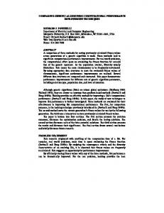
2.1. Dynamic time warping distance DTW is a dynamic programming algorithm that compares two series and tries to find the optimum warping path between them under certain constraints, such as monotonicity. It started being used by the data mining community to overcome some of the limitations associated with the Euclidean distance (Ratanamahatana and Keogh 2004; Berndt and Clifford 1994). The easiest way to get an intuition of what DTW does is graphically. Figure 1 shows the alignment between two sample time-series x and y. In this instance, the initial and final points of the series must match, but other points may be warped in time in order to find better matches. DTW is computationally expensive. If x has length n and y has length m, the DTW distance between them can be computed in O(nm) time, which is quadratic if m and n are similar. 4

1 0.5 0 −0.5

0.6 −0.4

−1

0.2

Series

0

50

100

150

Time

Figure 1: Sample alignment performed by the DTW algorithm between two series. The dashed blue lines exemplify how some points are mapped to each other, which shows how they can be warped in time. Note that the vertical position of each series was artificially altered for visualization.

Additionally, DTW is prone to implementation bias since its calculations are not easily vectorized and tend to be very slow in non-compiled programming languages. The dtw package (Giorgino 2009) includes a C implementation of the dynamic programming step of the algorithm, which should be very fast; its level of generality may sacrifice some performance, but in most situations it will be negligible. Optionally, a basic custom implementation of the DTW algorithm is included with dtwclust in the dtw_basic function, which has less functionality but still supports the most common options, it has a C++ core, implements some memory optimizations, and it is faster, especially when computing the DTW distance between several pairs of time-series. The DTW distance can potentially deal with series of different length directly. This is not necessarily an advantage, as it has been shown before that performing linear reinterpolation to obtain equal length may be appropriate if m and n do not vary significantly (Ratanamahatana and Keogh 2004). For a more detailed explanation of the DTW algorithm see, e.g., Giorgino (2009). However, there are some aspects that are worth discussing here. The first step in DTW involves creating a local cost matrix (LCM or lcm), which has n × m dimensions. Such a matrix must be created for every pair of series compared, meaning that memory requirements may grow quickly as the dataset size grows. Considering x and y as the input series, for each element (i, j) of the LCM, the lp norm between xi and yj must be computed. This is defined in Equation 1, explicitly denoting that multivariate series are supported as long as they have the same number of variables (note that for univariate series, the LCM will be identical regardless of the used norm). Thus, it makes sense to speak of a DTWp distance, where p corresponds to the lp norm that was used to construct the LCM. However, this norm also plays an important role in the next step of DTW. !1/p lcm(i, j) =

X |xvi − yjv |p v

5

(1)

In the seconds step, the DTW algorithm finds the path that minimizes the alignment between x and y by iteratively stepping through the LCM, starting at lcm(1, 1) and finishing at lcm(n, m), and aggregating the cost. At each step, the algorithm finds the direction in which the cost increases the least under the chosen constraints; see Figure 2 for a visual representation of the path corresponding to Figure 1. If we define φ = {(1, 1), . . . , (n, m)} as the set containing all the points that fall on the optimum path, then the final distance would be computed with Equation 2, where mφ is a per-step weighting coefficient and Mφ is the corresponding normalization constant (Giorgino 2009).

Timeseries alignment −0.5

xts −0.4 0.8

0

Reference index 50 100 d$index2

150

1.0

yts

0

50

d$index1 100 Query index

150

Figure 2: Visual representation of the optimum path found. The big square in the center represents the LCM created for these specific series.

DTWp (x, y) =

 X mφ lcm(k)p 1/p Mφ

, ∀k ∈ φ

(2)

In this definition the choice of lp norm comes into play twice during the DTW the algorithm. The dtw package also makes internal use of proxy to calculate the LCM, and it allows changing the norm by means of its dist.method argument. However, as previously mentioned, the norm only affects the LCM if multivariate series are used. By default, dtw does not consider the lp norm in Equation 2 during step two of the algorithm, regardless of what is provided in dist.method. For this reason, a special version of DTW2 is registered with proxy by dtwclust (called simply "DTW2"), which also uses dtw for the core calculations, but also uses the l2 norm in the second step. The dtw_basic function follows the above definition. The way in which the algorithm traverses through the LCM is primarily dictated by the chosen step pattern. It is a local constraint that determines which directions are allowed when moving ahead in the LCM as the cost is being aggregated, as well as the associated perstep weights. Figure 3 depicts two common step patterns and their names in the dtw package. 6

−1

1

0

●

1

●

●

−1

0

●

Query index

1

●

2

−1

1

Reference index

●

Reference index

0

Unfortunately, very few articles from the data mining community specify which pattern they use, although in the author’s experience, the symmetric1 pattern seems to be standard. By contrast, the dtw and dtw_basic functions use the symmetric2 pattern by default, but it is simple to modify this by providing the appropriate value in the step.pattern argument. The choice of step pattern also determines whether the corresponding DTW distance can be normalized or not (which may be important for series with different length). See Giorgino (2009) for a complete list of step patterns and to know which ones can be normalized.

1

●

●

−1

0 Query index

(a) symmetric1 step pattern

(b) symmetric2 step pattern

Figure 3: Two common step patterns used by DTW when traversing the LCM. At each step, the lines denote the allowed directions that can be taken, as well as the weight associated with each one.

It should be noted that the DTW distance does not satisfy the triangle inequality, and it is not symmetric in general, e.g., for asymmetric step patterns (Giorgino 2009). The patterns in Figure 3 can result in a symmetric DTW calculation, provided no constraints are used (see the next section), or all series have the same length if a constraint is indeed used.

Global DTW constraints One of the possible modifications of DTW is to use global constraints, also known as window constraints. These limit the area of the LCM that can be reached by the algorithm. There are many types of windows (see, e.g., Giorgino (2009)), but one of the most common ones is the Sakoe-Chiba window (Sakoe and Chiba 1978), with which an allowed region is created along the diagonal of the LCM (see Figure 4). These constraints can marginally speed up the DTW calculation, but they are mainly used to avoid pathological warping. It is common to use a window whose size is 10% of the series’ length, although sometimes smaller windows produce even better results (Ratanamahatana and Keogh 2004). Strictly speaking, if the series being compared have different lengths, a constrained path may not exist, since the Sakoe-Chiba band may prevent the end point of the LCM to be reached (Giorgino 2009). In these cases a slanted band window may be preferred, since it stays along the diagonal for series of different length and is equivalent to the Sakoe-Chiba 7

10 8 6 4 2

Reference: samples 1..10

2

4

6

8

10

Query: samples 1..10

Figure 4: Visual representation of the Sakoe-Chiba constraint for DTW. The red elements will not be considered by the algorithm when traversing the LCM.

window for series of equal length. If a window constraint is used with dtwclust, a slanted band is employed. It is not possible to know a priori what window size, if any, will be best for a specific application, although it is usually agreed that no constraint is a poor choice. For this reason, it is better to perform tests with the data one wants to work with, perhaps taking a subset to avoid excessive running times. It should be noted that, when reported, window sizes are always integers greater than zero. If we denote this number with w, and for the specific case of the slanted band window, the valid region of the LCM will be constituted by all valid points in the range [(i, j − w), (i, j + w)] for all (i, j) along the LCM diagonal. Thus, at each step, 2w + 1 elements will fall within the window for a given window size w. This is the convention followed by dtwclust.

Lower bounds for DTW Due to the fact that DTW itself is expensive to compute, lower bounds (LBs) for the DTW distance have been developed. These lower bounds guarantee being less than or equal to the corresponding DTW distance. They have been exploited when indexing time-series databases, classification of time-series, clustering, etc. (Keogh and Ratanamahatana 2005; Begum et al. 2015). Out of the existing DTW LBs, the two most effective are termed LB_Keogh (Keogh and Ratanamahatana 2005) and LB_Improved (Lemire 2009), and they have been implemented in dtwclust in the functions lb_keogh and lb_improved. The reader is referred to the respective articles for detailed definitions and proofs of the LBs, however some important considerations will be further discussed here. 8

Each LB can be computed with a specific lp norm. Therefore, it follows that the lp norms used for DTW and LB calculations must match, such that LBp ≤ DTWp . Moreover, LB Keoghp ≤ LB Improvedp ≤ DTWp , meaning that LB_Improved can provide a tighter LB. It must be noted that the LBs are only defined for series of equal length and are not symmetric regardless of the lp norm used to compute them. Also note that the choice of step pattern affects the value of the DTW distance, changing the tightness of a given LB.

0.0 −0.5

Series

0.5

1.0

One crucial step when calculating the LBs is the computation of the so-called envelopes. These envelopes require a window constraint, and are thus dependent on both the type and size of the window. Based on these, a running minimum and maximum are computed and, respectively, a lower and upper envelope are generated. Figure 5 depicts a sample time-series with its corresponding envelopes for a Sakoe-Chiba window of size 15.

0

50

100

150

Time

Figure 5: Visual representation of a time-series (shown as a solid black line) and its corresponding envelopes based on a Sakoe-Chiba window of size 15. The green dashed line represents the upper envelope, while the red dashed line represents the lower envelope.

When calculating the LBs between x and y, one must be taken as a reference and the other one as a query. Assume x is the reference and y is the query. First, a copy of the reference series is created; denote this copy with H. The envelopes for the query are computed: y’s upper and lower envelopes (UE and LE respectively) are compared against x, so that the values of H are updated according to Equation (3). Subsequently, LB_Keogh is defined as in Equation 4, where k·kp is the lp norm of the series. The improvement made by LB_Improved consists in calculating a second vector H 0 by using H as query and y as reference, effectively defining the LB as in Equation 5 (cf. Figure 5 in Lemire (2009)). Hi = U Ei ,

∀xi > U Ei

(3a)

Hj = LEj ,

∀xj < LEj

(3b)

LB Keoghp (x, y) = kx − Hkp LB Improvedp (x, y) =

q p LB Keoghp (x, y)p + LB Keoghp (y, H)p 9

(4) (5)

In order for the LBs to be worth it, they must be computed in significantly less time than it takes to calculate the DTW distance. Lemire (2009) developed a streaming algorithm to calculate the envelopes using no more than 3n comparisons when using a Sakoe-Chiba window. This algorithm has been ported to dtwclust using the C++ programming language, ensuring an efficient calculation, and it is exposed in the compute_envelope function. LB_Keogh requires the calculation of one set of envelopes for every pair of series compared, whereas LB_Improved must calculate two sets of envelopes for every pair of series. If the LBs must be calculated between several time-series, some envelopes can be reused when a given series is compared against many others. This optimization is included in the LB functions registered with proxy by dtwclust. The function dtw_lb included in dtwclust (and the corresponding version registered with proxy) leverages LB_Improved in order to find nearest neighbors faster. It first computes a distance matrix using only LB_Improved. Then, it looks for the nearest neighbor by taking the argument of the row-wise minima of the resulting matrix. Using this information, it updates the distance values of the nearest neighbors using the DTW distance. It continues this process iteratively until no changes in the nearest neighbors are detected. See Appendix C for specific examples. Because of the way it works, dtw_lb may only be useful if one is only interested in nearest neighbors, which is usually the case in partitional clustering. However, if partition around medoids is performed (see Section 3.2), the distance matrix should not be precomputed so that the matrices are correctly updated on each iteration. Additionally, a considerably large dataset would be needed before the overhead of DTW becomes much larger than that of dtw_lb’s iterations.

2.2. Global alignment kernel distance Cuturi (2011) proposed an algorithm to assess similarity between time series by using kernels. He began by formalizing an alignment between two series x and y as π, and defined the set of all possible alignments as A(n, m), which is constrained by the lengths of x and y. It is shown that the DTW distance can be understood as the cost associated with the minimum alignment as expressed in Equation (6), where |π| is the length of π and the divergence function ϕ is typically the Euclidean distance.

DTW(x,y) =

min π∈A(n,m)

Dx,y (π) =

|π| X

Dx,y (π)

(6a)




(6b)

ϕ xπ1 (i) , yπ2 (i)

i=1

A Global Alignment (GA) kernel is defined as in Equation 7, where κ is a local similarity function. In contrast to DTW, this kernel considers the cost of all possible alignments by computing their exponentiated soft-minimum, so it is argued that it quantifies similarities in a more coherent way. However, the GA kernel has associated limitations, namely diagonal dominance and a complexity O(nm). With respect to the former, Cuturi (2011) states that diagonal dominance should not be an issue as long as one of the series being compared is not 10

longer than twice the length of the other.

kGA (x,y) =

X

|π| Y

κ xπ1 (i) , yπ2 (i)




(7)

π∈A(n,m) i=1

In order to reduce the GA kernel’s complexity, Cuturi (2011) proposed using the triangular local kernel for integers shown in Equation 8, where T represents the kernel’s order. By combining it with the kernel κ in Equation (9) (which is based on the Gaussian kernel κσ ), the Triangular Global Alignment Kernel (TGAK) in Equation 10 is obtained. Such a kernel can be computed in O(T min(n, m)), and is parameterized by the triangular constraint T and the Gaussian’s kernel width σ.  ω(i, j) =

|i − j| 1− T

 (8) +

κ(x, y) = e−φσ (x,y)   kx−yk2 1 − 2 2 2σ φσ (x, y) = 2 kx − yk + log 2 − e 2σ TGAK(x, y, σ, T ) = τ

−1

  1 ω(i, j)κ(x, y) ω ⊗ κ (i, x; j, y) = 2 2 − ω(i, j)κ(x, y)

(9a) (9b)

(10)

The triangular constraint is similar to the window constraints that can be used in the DTW algorithm. When T = 0 or T → ∞, the TGAK converges to the original GA kernel. When T = 1, the TGAK becomes a slightly modified Gaussian kernel that can only compare series of equal length. If T > 1, then only the alignments that fulfil −T < π1 (i) − π2 (i) < T are considered. Cuturi (2011) also proposed a strategy to estimate the p value of σ based on the time-series themselves and their lengths, namely c · med(kx − yk) · med(|x|), where med(·) is the empirical median, c is some constant, and x and y are subsampled vectors from the dataset. This, however, introduces some randomness into the algorithm when the value of σ is not provided, so it might be better to estimate it once and re-use it in subsequent function evaluations. In dtwclust, the value of c is set to 1. The similarity returned by the TGAK can be normalized with Equation 11 so that its values lie in the range [0, 1]. Hence, a distance measure for time-series can be obtained by subtracting the normalized value from 1. The algorithm supports multivariate series and series of different length (with some limitations). The resulting distance is symmetric and satisfies the triangle inequality, although it is more expensive to compute in comparison to DTW.   log (TGAK(x, x, σ, T )) + log (TGAK(y, y, σ, T )) exp log (TGAK(x, y, σ, T )) − 2

(11)

A C implementation of the TGAK algorithm is available at its author’s website1 . An R wrapper has been implemented in dtwclust in the GAK function, performing the aforementioned 1

http://marcocuturi.net/GA.html, accessed on 2016-10-29

11

normalization and subtraction in order to obtain a distance measure that can be used in clustering procedures.

2.3. Soft-DTW Following with the idea of the TGAK, i.e., of regularizing DTW by smoothing it, Cuturi and Blondel (2017) proposed a unified algorithm using a parameterized soft-minimum as shown in Equation (12) (where ∆(x, y) represents the LCM), and called the resulting discrepancy a soft-DTW, discussing its differentiability. Thanks to this property, a gradient function can be obtained, and Cuturi and Blondel (2017) developed a more efficient way to compute it. This can be then used to calculate centroids with numerical optimization as discussed in Section 3.4.

dtwγ (x, y) = minγ {hA, ∆(x, y)i, A ∈ A(n, m)} ( mini≤n ai , γ = 0 minγ {a1 , . . . , an } = P −γ log ni=1 e−ai /γ , γ > 0

(12a) (12b)

However, as a stand-alone distance measure, the soft-DTW distance has some disadvantages: the distance can be negative, the distance between x and itself is not necessarily zero, it does not fulfill the triangle inequality, and also has quadratic complexity with respect to the series’ lengths. On the other hand, it is a symmetric distance, it supports multivariate series as well as different lengths, and it can provide differently smoothed results by means of a user-defined parameter γ.

2.4. Shape-based distance The shape-based distance (SBD) was proposed as part of the k -Shape clustering algorithm (Paparrizos and Gravano 2015); this algorithm will be further discussed in Section 3.5 and Section 4.2.2. SBD is presented as a faster alternative to DTW. It is based on the crosscorrelation with coefficient normalization (NCCc) sequence between two series, and is thus sensitive to scale, which is why Paparrizos and Gravano (2015) recommend z -normalization. The NCCc sequence is obtained by convolving the two series, so different alignments can be considered, but no point-wise warpings are made. The distance can be calculated with the formula shown in Equation 13, where k·k2 is the l2 norm of the series. Its range lies between 0 and 2, with 0 indicating perfect similarity. SBD(x, y) = 1 −

max (N CCc(x, y)) kxk2 kyk2

(13)

This distance can be efficiently computed by utilizing the Fast Fourier Transform (FFT) to obtain the NCCc sequence, which is how it is implemented in dtwclust in the SBD function, although that might make it sensitive to numerical precision, especially in 32-bit architectures. It can be very fast, it is symmetric, it was very competitive in the experiments performed in Paparrizos and Gravano (2015) (although the run-time comparison was slightly biased due to the slow MATLAB implementation of DTW), and it supports (univariate) series of different length directly. Additionally, some FFTs can be reused when computing the SBD between 12

several series; this optimization is also included in the SBD function registered with proxy by dtwclust.

2.5. Summary of distance measures The distances described in this section are the ones implemented in dtwclust, which serve as basis for the algorithms presented in Section 3 and Section 4. Table 1 summarizes the salient characteristics of these distances. Distance

Computational Normalized cost

Symmetric

Multivariate support

Support for length differences

LB Keogh

Low

No

No

No

No

LB Improved

Low

No

No

No

No

DTW

Medium

Can be*

Can be*

Yes

Yes

GAK

High

Yes

Yes

Yes

Yes

Soft-DTW

High

Yes

Yes

Yes

Yes

SBD

Low

Yes

Yes

No

Yes

Table 1: Characteristics of time-series distance measures implemented in dtwclust. Regarding the cells marked with an asterisk: the DTW distance can be normalized for certain step patterns, and can be symmetric for symmetric step patterns when either no window constraints are used, or all time-series have the same length if constraints are indeed used.

3. Time-series prototypes A very important step of time-series clustering has to do with the calculation of so-called time-series prototypes. It is expected that all series within a cluster are similar to each other, and one may be interested in trying to define a time-series that effectively summarizes the most important characteristics of all series in a given cluster. This series is sometimes referred to as an average series, and prototyping is also sometimes called time-series averaging, but we will prefer the term “prototyping”, although calling them time-series centroids is also common. Computing prototypes is commonly done as a sub-routine of a larger task. In the context of clustering (see Section 4), partitional procedures rely heavily on the prototyping function, since the resulting prototypes are used as cluster centroids. Prototyping could even be a preprocessing step, whereby different samples from the same source can be summarized before clustering (e.g., for the character trajectories dataset, all trajectories from the same character can be summarized and then groups of similar characters could be sought), thus reducing the amount of data and execution time. Another example is time-series classification based on nearest-neighbors, which can be optimized by considering only group-prototypes as neighbors instead of the union of all groups. Nevertheless, it is important to note that the distance used in the overall task should be congruent with the chosen centroid, e.g. using the DTW 13

distance for DTW-based prototypes. The choice of prototyping function is closely related to the chosen distance measure and, in a similar fashion, it is not simple to know which kind of prototype will be better a priori. There are several strategies available for time-series prototyping, although due to their high dimensionality, what exactly constitutes an average time-series is debatable, and some notions could worsen performance significantly. The following sections will briefly describe some of the common approaches, which are the ones implemented by default in dtwclust. Nevertheless, it is also possible to create custom prototyping functions and provide them in the centroid argument (see Section 8).

3.1. Mean and median The arithmetic mean is used very often in conjunction with the Euclidean distance, and in many applications this combination is very competitive, even with multivariate data. However, because of the structure of time-series, the mean is arguably a poor prototyping choice, and could even perturb convergence of a clustering algorithm (Petitjean et al. 2011). Mathematically, the mean simply takes the average of each time-point i across all variables of the considered time-series. For a cluster C of size N , the (possibly multivariate) time-series mean µ can be calculated with Equation 14, where xvc,i is the i-th element of the v-th variable from the c-th series that belongs to cluster C. µvi =

1 X v x , ∀c ∈ C N c c,i

(14)

Following this idea, it is also possible to use the median value across series in C instead of the mean, although we are not aware if this has been used in the existing literature. Also note that this prototype is limited to series of equal length and equal amount of variables.

3.2. Partition around medoids Another very common approach is to use partition around medoids (PAM). A medoid is simply a representative object from a cluster, in this case also a time-series, whose average distance to all other objects in the same cluster is minimal. Since the medoid object is always an element of the original data, PAM is sometimes preferred over mean or median so that the time-series structure is not altered. Another possible advantage of PAM is that, since the data does not change, it is possible to precompute the whole distance matrix once and re-use it on each iteration, and even across different number of clusters and random repetitions. While this precomputation is not necessary, it usually saves time overall, so it is done by default by dtwclust. However, this is not suitable for large datasets since the whole distance matrix has to be allocated at once, so it is also possible to deactivate this precomputation. In the implementation included in the package, k series from the data are randomly chosen as initial centroids. Then the distance between all series and the centroids is calculated (or retrieved from the whole distance matrix if it was precomputed), and each series is assigned to the cluster of its nearest centroid. For each created cluster, the distance between all member series is computed (if necessary), and the series with minimum sum of distances is chosen as 14

the new centroid. This continues iteratively until no series change clusters, or the maximum number of allowed iterations has been exceeded.

3.3. DTW barycenter averaging The DTW distance is used very often when working with time-series, and thus a prototyping function based on DTW has also been developed in Petitjean et al. (2011). The procedure is called DTW barycenter averaging (DBA), and is an iterative, global method. The latter means that the order in which the series enter the prototyping function does not affect the outcome. It is available as a standalone function in dtwclust, named simply DBA. DBA requires a series to be used as reference (centroid), and it usually begins by randomly selecting one of the series in the data. On each iteration, the DTW alignment between each series in the cluster C and the centroid is computed. Because of the warping performed in DTW, it can be that several time-points from a given time-series map to a single time-point in the centroid series, so for each time-point in the centroid, all the corresponding values from all series in C are grouped together according to the DTW alignments, and the mean is computed for each centroid point using the values contained in each group. This is iteratively repeated until a certain number of iterations are reached, or until convergence is assumed. The dtwclust implementation of DBA is done in C++ and includes several memory optimizations. Nevertheless, it is more computationally expensive due to all the DTW calculations that must be performed. However, it is very competitive when using the DTW distance and, thanks to DTW itself, it can support series with different length directly, with the caveat that the length of the resulting prototype will be the same as the length of the reference series that was initially chosen by the algorithm, and that the symmetric1 or symmetric2 step pattern should be used.

3.4. Soft-DTW centroid Thanks to the gradient that can be computed as a by-product of the soft-DTW distance calculation (see Section 2.3), it is possible to define an objective function (see Equation (4) in Cuturi and Blondel (2017)) and subsequently minimize it with numerical optimization. In addition to the smoothing parameter of soft-DTW (γ), the optimization procedure considers the option of using normalizing weights for the input series, which noticeably alters the resulting centroids (see Figure 4 in Cuturi and Blondel (2017)). The clustering and classification experiments performed by Cuturi and Blondel (2017) showed that using soft-DTW (distance and centroid) provided quantitatively better results in many scenarios.

3.5. Shape extraction A recently proposed method to calculate time-series prototypes is termed shape extraction, and is part of the k -Shape algorithm (see Section 4.2.2) described in Paparrizos and Gravano (2015); in dtwclust, it is implemented in the shape_extraction function. As with the corresponding SBD (see Section 2.4), the algorithm depends on NCCc, and it first uses it to match two series optimally. Figure 6 depicts the alignment that is performed using two sample series. As with DBA, a centroid series is needed, so one is usually randomly chosen from the data. An exception is when all considered time-series have the same length, in which case no centroid is 15

1.0 −1.5

0.0

Series

1.0 0.0

Series

−1.5 0

50

100

150

200

0

Time

50

100

150

200

Time

(a) Series before alignment

(b) Series after alignment

Figure 6: Visualization of the NCCc-based alignment performed on two sample series. After alignment, the second (red) series is either truncated and/or prepended/appended with zeros so that its length matches the first(black) series.

needed beforehand. The alignment can be done between series with different length, and since one of the series is shifted in time, it may be necessary to truncate and prepend or append zeros to the non-reference series, so that the final length matches that of the reference. This is because the final step of the algorithm builds a matrix with the matched series (row-wise) and performs a so-called maximization of Rayleigh Quotient to obtain the final prototype; see Paparrizos and Gravano (2015) for more details. The output series of the algorithm must be z -normalized. Thus, the input series as well as the reference series must also have this normalization. Even though the alignment can be done between series with different length, it has the same caveat as DBA, namely that the length of the resulting prototype will depend on the length of the chosen reference. Technically, for multivariate series, the shape extraction algorithm could be applied for each variable v of all involved series, but this was not explored by the authors of k -Shape.

3.6. Fuzzy-based prototypes Even though fuzzy clustering will not be discussed until Section 4.3, it is worth mentioning here that its most common implementation uses its own centroid function, which works like a weighted average. Therefore, it will only work with data of equal dimension, and it may not be suitable to use directly with raw time-series data.

3.7. Summary of prototyping functions Table 2 summarizes the time-series prototyping functions implemented in dtwclust, including the distance measure they are based upon, where applicable. It is worth mentioning that, as will be described in Section 4, the choice of distance and prototyping function is very important for time-series clustering, and it may be ill-advised to use a distance measure that does not correspond to the one used by the prototyping function. Using PAM is an exception, because the medoids are not modified, so any distance can be used to choose a medoid. It is possible to use custom prototyping functions for time-series clustering (see Section 8), but it is important to maintain congruence with the chosen distance measure.

16

Prototyping function

Distance used

Algorithm used

PAM

—

Time-series with minimum sum of distances to the other series in the group.

DBA

DTW

Average of points grouped according to DTW alignments.

Soft-DTW centroid

Soft-DTW

Shape extraction

SBD

Numerical optimization using the derivative of soft-DTW. Normalized eigenvector of a matrix created with SBD-aligned series.

Table 2: Time-series prototyping functions implemented in dtwclust, and their corresponding distance measures.

4. Time-series clustering algorithms 4.1. Hierarchical clustering Hierarchical clustering, as its name suggests, is an algorithm that tries to create a hierarchy of groups in which, as the level in the hierarchy increases, clusters are created by merging the clusters from the next lower level, such that an ordered sequence of groupings is obtained (Hastie et al. 2009). In order to decide how the merging is performed, a (dis)similarity measure between groups should be specified, in addition to the one that is used to calculate pairwise similarities. However, a specific number of clusters does not need to be specified for the hierarchy to be created, and the procedure is deterministic, so it will always give the same result for a chosen set of (dis)similarity measures. Algorithms for hierarchical clustering can be agglomerative or divisive, with the former being much more common than the latter (Hastie et al. 2009). In agglomerative procedures, every member of the data starts in its own cluster, and members are grouped together sequentially based on the similarity measure until all members are contained in a single cluster. Divisive procedures do the exact opposite, starting with all data in one cluster and dividing them until each member is in a singleton. Both strategies suffer from a lack of flexibility, because they cannot perform adjustments once a split or merger has been done. The intergroup dissimilarity is also known as linkage. As an example, single linkage takes the intergroup dissimilarity to be that of the closest (least dissimilar) pair (Hastie et al. 2009). There are many linkage methods available, although if the data can be “easily” grouped, they should all provide similar results. In dtwclust, the native R function hclust is used by default, and all its linkage methods are supported. However, it is possible to use other clustering functions, albeit with some limitations (see Appendix D). 17

The created hierarchy can be visualized as a binary tree where the height of each node is proportional to the value of the intergroup dissimilarity between its two daughter nodes (Hastie et al. 2009). Such a plot is called a dendrogram, an example of which can be seen in Figure 7. These plots can be a useful way of summarizing the whole data in an interpretable way, although it may be deceptive, as the algorithms impose the hierarchical structure even if such structure is not inherent to the data (Hastie et al. 2009).

M.V1 N.V1 H.V2 H.V4 H.V5 H.V1 H.V3 N.V5 N.V2 N.V3 W.V2 W.V3 W.V5 N.V4 W.V4 G.V3 G.V5 Y.V3 Y.V1 Y.V2 Y.V4 Y.V5 B.V1 B.V5 P.V1 P.V2 P.V4 P.V3 P.V5 B.V4 B.V2 B.V3 O.V1 O.V5 O.V2 O.V3 O.V4 S.V1 S.V4 S.V2 S.V3 S.V5 G.V2 G.V1 G.V4 R.V3 R.V1 R.V2 E.V5 E.V3 E.V1 E.V2 E.V4 R.V4 R.V5 L.V1 L.V3 L.V4 L.V2 L.V5 C.V3 C.V2 C.V5 C.V1 C.V4 Z.V3 Z.V2 Z.V4 Z.V5 Z.V1 Q.V1 Q.V2 Q.V5 Q.V3 Q.V4 A.V3 A.V4 A.V5 A.V1 A.V2 U.V1 D.V5 D.V3 D.V4 D.V1 D.V2 U.V2 U.V3 U.V4 U.V5

V.V3 V.V5 V.V4 V.V1 V.V2 M.V2 M.V5 M.V3 M.V4

W.V1

0.2 0.0

0.1

Height

0.3

0.4

0.5

Cluster Dendrogram

stats::as.dist(distmat) stats::hclust (*, "average")

Figure 7: Sample dendrogram created by using SBD and average linkage.

The dendrogram does not directly imply a certain number of clusters, but one can be induced. One option is to visually evaluate the dendrogram in order to assess the height at which the largest change in dissimilarity occurs, consequently cutting the dendrogram at said height and extracting the clusters that are created. Another option is to specify the number of clusters that are desired, and cut the dendrogram in such a way that the chosen number is obtained. In the latter case, several cuts can be made, and validity indices can be used to decide which value yields better performance (see Section 6). Once the clusters have been obtained, it may be desirable to use them to create prototypes (see Section 3). At this point, any suitable prototyping function may be used, but we want to emphasize that this is not a mandatory step in hierarchical clustering. A complete set of examples is provided in Appendix D. Hierarchical clustering has the disadvantage that the whole distance matrix must be calculated for a given dataset, which in most cases has a time and memory complexity of O(N 2 ) if N is the total number of objects in the dataset. Thus, hierarchical procedures are usually used with relatively small datasets.

4.2. Partitional clustering Partitional clustering is a different strategy used to create partitions. In this case, the data 18

is explicitly assigned to one and only one cluster out of k total clusters. The total number of desired clusters must be specified beforehand, which can be a limiting factor, although this can be ameliorated by using validity indices (see Section 6). Partitional procedures can be stated as combinatorial optimization problems that minimize the intracluster distance while maximizing the intercluster distance. However, finding a global optimum would require enumerating all possible groupings, something which is infeasible even for relatively small datasets (Hastie et al. 2009). Therefore, iterative greedy descent strategies are used instead, which examine a small fraction of the search space until convergence, but could converge to local optima. Partitional clustering algorithms commonly work in the following way. First, k centroids are randomly initialized, usually by choosing k objects from the dataset at random; these are assigned to individual clusters. The distance between all objects in the data and all centroids is calculated, and each object is assigned to the cluster of its closest centroid. A prototyping function is applied to each cluster to update the corresponding centroid. Then, distances and centroids are updated iteratively until a certain number of iterations have elapsed, or no object changes clusters any more. It can happen that a cluster becomes empty at a certain iteration, in which case a new cluster can be reinitialized at random by choosing a new object from the data (this is what dtwclust does). This tries to maintain the desired amount of clusters, but can result in instability or divergence in some cases. Perhaps using a different distance function or a lower value of k can help in those situations. An optimization that the included centroid functions in dtwclust have is that, on each iteration, the centroid function is only applied to those clusters that changed either by losing or gaining data objects. Additionally, when PAM centroids are used and the distance matrix is precomputed, the function simply keeps track of the data indices, how they change, and which ones are chosen as cluster centroids, so that no data is modified. Some of the most popular partitional algorithms are k -means and k -medoids (Hastie et al. 2009). These use the Euclidean distance and, respectively, mean or PAM centroids (see Section 3). Most of the proposed algorithms for time-series clustering use the same basic strategy while changing the distance and/or centroid function. Partitional clustering procedures are stochastic due to their random start. Thus, it is common practice to test different random starts to evaluate several local optima and choose the best result out of all the repetitions. It tends to produce spherical clusters, but has a lower complexity, so it can be applied to very large datasets. An example is given in Appendix E.

TADPole clustering TADPole clustering was proposed in Begum et al. (2015), and is implemented in dtwclust in the TADPole function. It adopts a relatively new clustering framework and adapts it to time-series clustering with the DTW distance. Because of the way the algorithm works, it can be considered a kind of PAM clustering, since the centroids are always elements of the data. However, this algorithm is deterministic depending on the value of a cutoff distance (dc ). The algorithm first uses the DTW distance’s upper and lower bounds (Euclidean distance and LB_Keogh respectively) to find series with many close neighbors (in DTW space). Anything below dc is considered a neighbor. Aided with this information, the algorithm then tries to prune as many DTW calculations as possible in order to accelerate the clustering procedure. The series that lie in dense areas (i.e., that have lots of neighbors) are taken as cluster 19

centroids. For a more detailed explanation of each step, please refer to Begum et al. (2015). TADPole relies on the DTW bounds, which are only defined for time-series of equal length. Consequently, it requires a Sakoe-Chiba constraint. Furthermore, it should be noted that the Euclidean distance is only valid as a DTW upper bound if the symmetric1 step pattern is used (see Figure 3). Finally, the allocation of several distance matrices is required, making it similar to hierarchical procedures memory-wise, so its applicability is limited to relatively small datasets.

k-Shape clustering The k -Shape clustering algorithm was developed by Paparrizos and Gravano (2015). It is a partitional clustering algorithm with a custom distance measure (SBD; see Section 2.4), as well as a custom centroid function (shape extraction; see Section 3.5). It is also stochastic in nature, and requires z -normalization in its default definition. Both the distance and centroid functions were implemented in dtwclust as individual functions, because that allows the user to combine them and use them independently with other algorithms. In order to use this clustering algorithm, the main clustering function (tsclust) should be called with SBD as the distance measure, shape extraction as the centroid function, and z -normalization as the preprocessing step.

4.3. Fuzzy clustering The previous procedures result in what is known as a crisp or hard partition, although hierarchical clustering only indirectly when the dendrogram is cut. In crisp partitions, each member of the data belongs to only one cluster, and clusters are mutually exclusive. By contrast, fuzzy clustering creates a fuzzy or soft partition in which each member belongs to each cluster to a certain degree. For each member of the data, the degree of belongingness is constrained so that its sum equals 1 across all clusters. Therefore, if there are N objects in the data and k clusters are desired, an N × k membership matrix u can be created, where all the rows must sum to 1 (note that some authors use the transposed version of u). One of the most widely used versions of the algorithm is fuzzy c-means, which is described in Bezdek (1981), and is implemented in dtwclust. It tries to create a fuzzy partition by minimizing the function in Equation (15a) under the constraints given in Equation (15b). The membership matrix u is initialized randomly in such a way that the constraints are fulfilled. The exponent m is known as the fuzziness exponent and should be greater than 1, with a common default value of 2. Originally, the distance dp,c was defined as the Euclidean distance between the p-th object and the c-th fuzzy centroid, so that the objective was written in terms of the squared Euclidean distance. However, the definition of this distance can change (see, e.g., D’Urso and Maharaj (2009)), and, in contrast to other R packages that implement fuzzy clustering, doing so in dtwclust is straightforward, since it only entails registering the 20

corresponding distance function with proxy.

min

N X k X

2 um p,c dp,c

(15a)

p=1 c=1 k X

up,c ≥ 0

up,c = 1,

(15b)

c=1

The centroid function used by fuzzy c-means calculates the mean for each point across all members in the data, weighted by their degree of belongingness. If we define µc,i as the i-th element of the c-th centroid, and xp,i as the i-th data-point of the p-th object in the data, the centroid calculation can be expressed with Equation 16. It follows that all members of the data must have the same dimensionality in this case. As with the normal mean prototype, this centroid function might not be suitable for time-series, so it might be better to first apply a transformation to the data and cluster in the resulting space. For instance, D’Urso and Maharaj (2009) used the autocorrelation function to extract a certain amount of coefficients from time-series, resulting in data with equal dimensionality, and performed fuzzy clustering on the autocorrelation coefficients. See Appendix F for an example. PN

m p=1 up,c xp,i m p=1 up,c

µc,i =

(16)

PN

Another option is to use fuzzy c-medoids (FCMdd) as the centroid function (Krishnapuram et al. 2001; Izakian et al. 2015), whereby the centroids are selected according to Equation (17). Similar to PAM, this centroid function does not alter the data, so the centroids are always elements of the original set, and series of different length can be supported (as long as the distance function also supports this).

µc = x q q = arg min

N X

(17a) 2 um p,c dp,c

(17b)

p=1

Finally, the objective is minimized iteratively by applying Equation 18 a certain number of iterations or until convergence is assumed. In Equation 18, dp,c represents the distance between the p-th member of the data and the c-th fuzzy centroid, so great care must be given to the shown indices p, c and q. It is clear from the equation that this update only depends on the chosen fuzziness exponent and the distance measure. up,c =

1 2 m−1

dp,c

Pk

q=1



1



2 m−1

(18)

dp,q

Technically, fuzzy clustering can be repeated several times with different random starts, since u is initialized randomly. However, comparing the results would be difficult, since it could 21

be that the values within u are shuffled but the overall fuzzy grouping remains the same, or changes very slightly, once the algorithm has converged. Note that it is straightforward to change the fuzzy partition to a crisp one by taking the argument of the row-wise maxima of u or of the row-wise minima of dp,c for all p, and assigning the respective series to the corresponding cluster only.

5. Parallel computation Using parallelization is not something that is commonly explored explicitly in the literature, but it can be extremely useful in practical applications. In the case of time-series clustering, parallel computation can result in a very significant reduction in execution times. There are some important considerations when using parallelization. First of all, there is a basic distinction between multi-process and multi-threaded parallelization. The optimal amount of parallel workers, i.e., subprocesses that can each handle a given task, is dependent on the computer processor that is being used and the number of physical processing cores and logical threads it can handle. Each worker may require additional RAM, and R usually only works with data that is loaded on RAM. Finally, the overhead introduced for the orchestration of parallelization may be too large when compared to the amount of time needed to complete each task, which is especially true for relatively simple workloads. Therefore, using parallelization does not guarantee faster execution times, and should be tested in the context of a specific application. Handling parallelization has been greatly simplified in R by different software packages. The implementations done in dtwclust use the foreach package (Revolution Analytics and Weston 2017) for multi-processing, and RcppParallel for multi-threading (Allaire et al. 2018). See Appendix G for a specific example of multi-processing, and refer to the parallelization vignette for additional information. The documentation for each function specifies if they use parallelization and how, but in general, all distances included with dtwclust use multi-threading, and multi-processing is leveraged during clustering. Before describing the different cases where dtwclust can take advantage of multi-processing, it should also be noted that, by default, there is only one level of parallelization in that case. This means that all tasks performed by a given parallel worker’s process are done sequentially, and they cannot take advantage of further parallelization even if there are workers available. When performing partitional clustering, it is common to do many repetitions with different random seeds to account for different starting points. When many repetitions are specified directly to tsclust, the package assigns each repetition to a different worker. This is also the case when the function is called with several values of k, i.e., when different number of clusters are to be tested; this is detected in partitional, fuzzy and TADPole clustering. The included implementation of the TADPole algorithm also supports multi-processing for different values of the cutoff distance. In the context of partitional clustering, calculating time-series prototypes is something that is done many times each iteration. Since clusters are mutually exclusive, the prototype calculations can be executed in parallel, but this is only worth it if the calculations are time consuming. Therefore, in dtwclust, only DBA, shape extraction, and the soft-DTW centroid attempt to do multi-processing when used in partitional clustering. 22

6. Cluster evaluation Clustering is commonly considered to be an unsupervised procedure, so evaluating its performance can be rather subjective. However, a great amount of effort has been invested in trying to standardize cluster evaluation metrics by using cluster validity indices (CVIs). Many indices have been developed over the years, and they form a research area of their own, but there are some overall details that are worth mentioning. The discussion here is based on Arbelaitz et al. (2013) and Wang and Zhang (2007), which provide a much more comprehensive overview. In general, CVIs can be either tailored to crisp or fuzzy partitions. For the former, CVIs can be classified as internal, external or relative depending on how they are computed. Focusing on the first two, the crucial difference is that internal CVIs only consider the partitioned data and try to define a measure of cluster purity, whereas external CVIs compare the obtained partition to the correct one. Thus, external CVIs can only be used if the ground truth is known. Note that even though a fuzzy partition can be changed into a crisp one, making it compatible with many of the existing “crisp” CVIs, there are also fuzzy CVIs tailored specifically to fuzzy clustering, and these may be more suitable in those situations. Fuzzy partitions usually have no ground truth associated with them, but there are exceptions depending on the task’s goal (Lei et al. 2017). Each index defines its range of values and whether they are to be minimized or maximized. In many cases, these CVIs can be used to evaluate the result of a clustering algorithm regardless of how the clustering works internally, or how the partition came to be. The Silhouette index (Rousseeuw 1987) is an example of an internal CVI, whereas the Variation of Information (Meil˘a 2003) is an external CVI. Several of the best-performing CVIs according to Wang and Zhang (2007), Arbelaitz et al. (2013), and Lei et al. (2017) are implemented in dtwclust in the cvi function. Table 3 specifies which ones are available and some of their particularities. There are some advantages and corresponding caveats with respect to the dtwclust implementations. Many internal CVIs require additional distance calculations, and some also compute so-called global centroids (a centroid that uses the whole dataset), which were calculated with, respectively, the Euclidean distance and a mean centroid in the original definition. The implementations in dtwclust change this, making use of whatever distance/centroid was utilized during clustering without further intervention from the user, so it is possible to leverage the distance and centroid functions that support time-series. Nevertheless, many CVIs assume symmetric distance functions, so the cvi function warns the user when this is not fulfilled. Knowing which CVI will work best cannot be determined a priori, so they should be tested for each specific application. Many CVIs can be utilized and compared to each other, maybe using a majority vote to decide on a final result, but there is no best CVI, and it is important to conceptually understand what a given CVI measures in order to appropriately interpret its results. Furthermore, it should be noted that, due to additional distance and/or centroid calculations, computing CVIs can be prohibitive in some cases. For example, the Silhouette index effectively needs the whole distance matrix between the original series to be calculated. CVIs are not the only way to evaluate clustering results. The clue package (Hornik 2005, 2017) includes its own extensible framework for evaluation of cluster ensembles. It does not directly 23

CVI

Internal or external

Crisp or fuzzy partitions

Minimized or Maximized

Considerations

Rand

External

Crisp

Maximized

—

Adjusted rand

External

Crisp

Maximized

—

Jaccard

External

Crisp

Maximized

—

Fowlkes-Mallows

External

Crisp

Maximized

—

Variation of information

External

Crisp

Minimized

—

Soft rand

External

Fuzzy

Maximized

—

Soft adjusted rand

External

Fuzzy

Maximized

—

Soft variation of information

External

Fuzzy

Minimized

—

Soft normalized mutual information

External

Fuzzy

Maximized

—

Silhouette

Internal

Crisp

Maximized

Requires the whole cross-distance matrix.

Dunn

Internal

Crisp

Maximized

Requires the whole cross-distance matrix.

COP

Internal

Crisp

Minimized

Requires the whole cross-distance matrix.

Davies-Bouldin

Internal

Crisp

Minimized

Calculates distances to the computed cluster centroids.

Modified Davies-Bouldin (DB*)

Internal

Crisp

Minimized

Calculates distances to the computed cluster centroids.

Calinski-Harabasz

Internal

Crisp

Maximized

Calculates a global centroid.

Score function

Internal

Crisp

Maximized

Calculates a global centroid.

MPC

Internal

Fuzzy

Maximized

—

K

Internal

Fuzzy

Minimized

Calculates a global centroid.

T

Internal

Fuzzy

Minimized

—

SC

Internal

Fuzzy

Maximized

Calculates a global centroid.

PBMF

Internal

Fuzzy

Maximized

Calculates a global centroid.

Table 3: Cluster validity indices included in dtwclust. Internal fuzzy CVIs use the nomenclature from Wang and Zhang (2007).

24

deal with the clustering algorithms themselves, rather with ways of quantifying agreement and consensus between several clustering results. As such, it is directly compatible with the results from dtwclust, since it does not care how a partition/hierarchy was created. Support for the clue package framework is included, see Appendix H for more complete examples.

7. Comparing clustering algorithms with dtwclust As we have seen, there are several aspects that must be considered for time-series clustering. Some examples are: • Pre-processing of data, possibly changing the decision space. • Type of clustering (partitional, hierarchical, etc.). • Number of desired or expected clusters. • Choice of distance measure, along with its parameterization. • Choice of centroid function and its parameterization. This may also depend on the chosen distance. • Evaluation of clustering results. • Computational cost, which depends not only on the size of the dataset, but also on the complexity of the aforementioned aspects. In order to facilitate more laborious workflows, dtwclust includes the compare_clusterings function which, along with its helper functions, optimizes the way the different clustering algorithms can be executed. Its main advantage is that it leverages parallelization. In order to avoid data copies and communication overhead in these scenarios, compare_clusterings is coded in a way that, by default, less data is returned from the parallel processes. Nevertheless, as is shown in Appendix I, the results can be fully re-created in the main process on demand. With this infrastructure, it is possible to cover the whole clustering workflow with dtwclust.

8. Package extensibility All of the clustering algorithms implemented in dtwclust have something in common: they depend on a distance measure between time-series. By leveraging the proxy package, any suitable distance function can be used (see Appendix B). This fact alone already overcomes a severe limitation that other packages have, such as flexclust (Leisch 2006). Another important aspect of the clustering procedure is the extraction of centroids or timeseries prototypes. The most common ones are already implemented in dtwclust, but it is also possible to provide custom centroid algorithms (see Appendix J). Because of this, it would even be possible to implement a custom fuzzy clustering algorithm if desired. As previously mentioned, most time-series clustering algorithms use existing functions and only modify the distance and centroid functions to an appropriate one. On the other hand, a lot of work has also been devoted to time-series representation. However, performing data 25

transformations can be done independently of dtwclust, or provided as a preprocessing function if desired (which might be more convenient if the predict generic is to be used). Other clustering algorithms that make significant modifications would be harder to integrate by the user. However, it would still be possible, thanks to the open-source nature of R and the fact that dtwclust is hosted on GitHub2 .

9. Conclusion In this manuscript a general overview of shape-based time-series clustering was provided. This included a lot of information related to the DTW distance and its corresponding optimizations, such as constraints and lower bounding techniques. At the same time, the dtwclust package for R was described and showcased, demonstrating how it can be used to test and compare different procedures efficiently and unbiasedly by providing a common infrastructure. The package implements several different routines, most of which are related to the DTW algorithm. Nevertheless, its modular structure enables the user to customize and complement the included functionality by means of custom algorithms or even other R packages, as it was the case with TSdist, cluster and clue. These packages are more specialized, dealing with specific tasks (respectively: distance calculations, hierarchical clustering, cluster evaluation), and they are more difficult to extend. By contrast, dtwclust provides a more general purpose clustering workflow, having enough flexibility to allow for the most common approaches to be used. The goal of this manuscript was not to give a comprehensive and thorough explanation of all the discussed algorithms, but rather to provide information related to what has been done in the literature, including some more recent propositions, so that the reader knows where to start looking for further information, as well as what can or cannot be done with dtwclust. Choosing a specific clustering algorithm for a given application is not an easy task. There are many factors to take into account and it is not possible to know a priori which one will yield the best results. The included implementations try to use the native (and heavily optimized) R functions as much as possible, relying on compiled code where needed, so we hope that, if time-series clustering is required, dtwclust can serve as a starting point.

2

https://github.com/asardaes/dtwclust

26

References Aggarwal CC, Hinneburg A, Keim DA (2001). “On the Surprising Behavior of Distance Metrics in High Dimensional Space.” In JV den Bussche, V Vianu (eds.), International Conference on Database Theory, pp. 420–434. Springer-Verlag. Aggarwal CC, Reddy CK (2013). “Time-Series Data Clustering.” In Data Clustering: Algorithms and Applications, chapter 15. CRC Press. Aghabozorgi S, Shirkhorshidi AS, Wah TY (2015). “Time-Series Clustering — A Decade Review.” Information Systems, 53, 16–38. URL https://doi.org/10.1016/j.is.2015. 04.007. Allaire J, Francois R, Ushey K, Vandenbrouck G, Geelnard M, Intel (2018). RcppParallel: Parallel Programming Tools for ’Rcpp’. R package version 4.4.0, URL https://CRAN. R-project.org/package=RcppParallel. Arbelaitz O, Gurrutxaga I, Muguerza J, P´erez JM, Perona I (2013). “An Extensive Comparative Study of Cluster Validity Indices.” Pattern Recognition, 46(1), 243–256. URL https://doi.org/10.1016/j.patcog.2012.07.021. Begum N, Ulanova L, Wang J, Keogh E (2015). “Accelerating Dynamic Time Warping Clustering with a Novel Admissible Pruning Strategy.” In Conference on Knowledge Discovery and Data Mining, KDD ’15. ACM. ISBN 978-1-4503-3664-2/15/08. URL https://doi.org/10.1145/2783258.2783286. Berndt DJ, Clifford J (1994). “Using Dynamic Time Warping to Find Patterns in Time Series.” In KDD Workshop, volume 10, pp. 359–370. Seattle, WA. Bezdek JC (1981). Pattern Recognition with Fuzzy Objective Function Algorithms. Kluwer Academic Publishers. Brandmaier AM (2015). “pdc: An R Package for Complexity-Based Clustering of Time Series.” Journal of Statistical Software, 67(5), 1–23. URL https://doi.org/10.18637/ jss.v067.i05. Cuturi M (2011). “Fast Global Alignment Kernels.” In Proceedings of the 28th international conference on machine learning (ICML-11), pp. 929–936. Cuturi M, Blondel M (2017). “Soft-DTW: a Differentiable Loss Function for Time-Series.” In D Precup, YW Teh (eds.), Proceedings of the 34th International Conference on Machine Learning, volume 70 of Proceedings of Machine Learning Research, pp. 894–903. PMLR, International Convention Centre, Sydney, Australia. URL http://proceedings.mlr.press/ v70/cuturi17a.html. Dau HA, Begum N, Keogh E (2016). “Semi-supervision dramatically improves time series clustering under dynamic time warping.” In Proceedings of the 25th ACM International on Conference on Information and Knowledge Management, pp. 999–1008. ACM. URL https://doi.org/10.1145/2983323.2983855. 27

D’Urso P, Maharaj EA (2009). “Autocorrelation-Based Fuzzy Clustering of Time Series.” Fuzzy Sets and Systems, 160(24), 3565–3589. URL https://doi.org/10.1016/j.fss. 2009.04.013. Giorgino T (2009). “Computing and Visualizing Dynamic Time Warping Alignments in R: The dtw Package.” Journal of Statistical Software, 31(7), 1–24. URL https://doi.org/ 10.18637/jss.v031.i07. Hastie T, Tibshirani R, Friedman J (2009). “Cluster Analysis.” In The Elements of Statistical Learning 2nd Edition, chapter 14.3. New York: Springer-Verlag. Hornik K (2005). “A CLUE for CLUster Ensembles.” Journal of Statistical Software, 14(12), 1–25. URL https://doi.org/10.18637/jss.v014.i12. Hornik K (2017). clue: Cluster Ensembles. R package version 0.3-54, URL https://CRAN. R-project.org/package=clue. Izakian H, Pedrycz W, Jamal I (2015). “Fuzzy clustering of time series data using dynamic time warping distance.” Engineering Applications of Artificial Intelligence, 39, 235–244. URL https://doi.org/10.1016/j.engappai.2014.12.015. Kaufman L, Rousseeuw PJ (1990). Finding Groups in Data. An Introduction to Cluster Analysis, volume 1, chapter 1. John Wiley & Sons. Keogh E, Ratanamahatana CA (2005). “Exact Indexing of Dynamic Time Warping.” Knowledge and information systems, 7(3), 358–386. URL https://doi.org/10.1007/ s10115-004-0154-9. Krishnapuram R, Joshi A, Nasraoui O, Yi L (2001). “Low-complexity fuzzy relational clustering algorithms for web mining.” IEEE transactions on Fuzzy Systems, 9(4), 595–607. URL https://doi.org/10.1109/91.940971. Lei Y, Bezdek JC, Chan J, Vinh NX, Romano S, Bailey J (2017). “Extending informationtheoretic validity indices for fuzzy clustering.” IEEE Transactions on Fuzzy Systems, 25(4), 1013–1018. URL https://doi.org/10.1109/TFUZZ.2016.2584644. Leisch F (2006). “A Toolbox for k-Centroids Cluster Analysis.” Computational Statistics & Data Analysis, 51(2), 526–544. URL https://doi.org/10.1016/j.csda.2005.10.006. Lemire D (2009). “Faster Retrieval with a Two-Pass Dynamic-Time-Warping Lower Bound.” Pattern Recognition, 42(9), 2169 – 2180. ISSN 0031-3203. URL https://doi.org/10. 1016/j.patcog.2008.11.030. Liao TW (2005). “Clustering of Time Series Data: A Survey.” Pattern recognition, 38(11), 1857–1874. URL https://doi.org/10.1016/j.patcog.2005.01.025. Lichman M (2013). “UCI Machine Learning Repository.” URL http://archive.ics.uci. edu/ml. Maechler M, Rousseeuw P, Struyf A, Hubert M, Hornik K (2017). cluster: Cluster Analysis Basics and Extensions. R package version 2.0.6, URL https://CRAN.R-project.org/ package=cluster. 28

Meil˘a M (2003). “Comparing Clusterings by the Variation of Information.” In Learning Theory and Kernel Machines, pp. 173–187. Springer-Verlag. URL https://doi.org/10. 1007/978-3-540-45167-9_14. Meyer D, Buchta C (2018). proxy: Distance and Similarity Measures. R package version 0.4-21, URL https://CRAN.R-project.org/package=proxy. Microsoft Corporation, Weston S (2017). doParallel: Foreach Parallel Adaptor for the ’parallel’ Package. R package version 1.0.11, URL https://CRAN.R-project.org/package= doParallel. Montero P, Vilar JA (2014). “TSclust: An R Package for Time Series Clustering.” Journal of Statistical Software, 62(1), 1–43. URL https://doi.org/10.18637/jss.v062.i01. Mori U, Mendiburu A, Lozano JA (2016). “Distance Measures for Time Series in R: The TSdist Package.” R Journal, 8(2), 451–459. URL https://journal.r-project.org/ archive/2016/RJ-2016-058/index.html. Paparrizos J, Gravano L (2015). “k-Shape: Efficient and Accurate Clustering of Time Series.” In Proceedings of the 2015 ACM SIGMOD International Conference on Management of Data, SIGMOD ’15, pp. 1855–1870. ACM, New York, NY, USA. ISBN 978-1-4503-2758-9. URL https://doi.org/10.1145/2949741.2949758. Petitjean F, Ketterlin A, Gan¸carski P (2011). “A Global Averaging Method for Dynamic Time Warping, with Applications to Clustering.” Pattern Recognition, 44(3), 678 – 693. ISSN 0031-3203. URL https://doi.org/10.1016/j.patcog.2010.09.013. R Core Team (2018). R: A Language and Environment for Statistical Computing. R Foundation for Statistical Computing, Vienna, Austria. URL https://www.R-project.org/. Rani S, Sikka G (2012). “Recent Techniques of Clustering of Time Series Data: A Survey.” International Journal of Computer Applications, 52(15). URL https://doi.org/10.5120/ 8282-1278. Ratanamahatana CA, Keogh E (2004). “Everything you know about dynamic time warping is wrong.” In Third workshop on mining temporal and sequential data. Citeseer. Revolution Analytics, Weston S (2017). foreach: Provides Foreach Looping Construct for R. R package version 1.4.4, URL https://CRAN.R-project.org/package=foreach. Rousseeuw PJ (1987). “Silhouettes: a graphical aid to the interpretation and validation of cluster analysis.” Journal of computational and applied mathematics, 20, 53–65. URL https://doi.org/10.1016/0377-0427(87)90125-7. Sakoe H, Chiba S (1978). “Dynamic Programming Algorithm Optimization for Spoken Word Recognition.” Acoustics, Speech and Signal Processing, IEEE Transactions on, 26(1), 43– 49. ISSN 0096-3518. URL https://doi.org/10.1109/TASSP.1978.1163055. Wang W, Zhang Y (2007). “On fuzzy cluster validity indices.” Fuzzy sets and systems, 158(19), 2095–2117. URL https://doi.org/10.1016/j.fss.2007.03.004.

29

A. Technical notes After installation, the package and the sample data can be loaded and attached with the following code. library("dtwclust") data("uciCT") The main clustering function is tsclust. It returns objects of type S4, which are one way in which R implements classes. The formal elements of the class are called slots, and can be accessed with the @ operator (instead of the usual $). The documentation of the slots can be found with ?"TSClusters-class", and the methods with ?"TSClusters-methods". Controls are set via intermediary functions whose documentation can be found by typing ?"tsclust-controls". The function compare_clusterings and its helper functions can be used to execute many different clustering configurations in a convenient way. The tsclust function is used for the calculations. A series of examples are included in the documentation of the function. The random number generator of R is set to L’Ecuyer-CMRG when dtwclust is attached3 in an attempt to preserve reproducibility. The user is free to change this afterwards by using the RNGkind function. This manuscript summarizes some of the theory behind the algorithms. However, the documentation of the different functions and the other vignettes4 include additional information regarding usability, and should also be considered when using the package.

B. Using the proxy package The proxy package is one of the main dependencies of dtwclust. It aggregates all its measures in a database object called pr_DB. This has the advantage that all registered functions can be used with the proxy::dist function, which results in a high level of consistency. Moreover, this also means that distance measures from dtwclust, other R packages, or user-created can be exploited in different applications, even those that are not directly related to time-series clustering. All the distances mentioned in this manuscript are registered with proxy when dtwclust is attached in R. It is important to note that the proxy::dist function parses all matrix-like objects row-wise, meaning that, in the context of time-series clustering, it would consider the rows of a matrix or data frame as the individual time-series. Matrices and data frames cannot contain series with different length, something that can be circumvented by encapsulating the series in a list, each element of the list being a single series. Internally, dtwclust coerces all provided data to a list, and it parses both matrices and data frames row-wise (see function tslist). Moreover, lists enable support for multivariate series, where a single multivariate time-series should be provided as a matrix where time spans the rows and the variables span the columns. Thus, several multivariate time-series should be provided as a list of matrices to ensure that they are correctly detected. Note, however, that not all distance and centroid functions support multivariate time-series. 3 4

Via the library function. Loading without attaching the package would not change the generator. https://cran.r-project.org/web/packages/dtwclust/vignettes/

30

As a first example, the autocorrelation-based distance from the TSclust package (Montero and Vilar 2014) is registered with proxy so that it can be used either directly or with dtwclust. require("TSclust") proxy::pr_DB$set_entry(FUN = diss.ACF, names = c("ACFD"), loop = TRUE, type = "metric", distance = TRUE, description = "Autocorrelation-based distance") # Taking just a subset of the data # Note that subsetting with single brackets preserves the list format proxy::dist(CharTraj[3:8], method = "ACFD", upper = TRUE) ## ## ## ## ## ## ##

A.V3 A.V3 A.V4 A.V5 B.V1 B.V2 B.V3

0.7347970 0.7269654 1.3365966 0.9022004 0.6204877

A.V4 A.V5 0.7347970 0.7269654 0.2516642 0.2516642 2.0014314 2.0178486 1.5712718 1.6136650 1.2133404 1.2901999

B.V1 B.V2 B.V3 1.3365966 0.9022004 0.6204877 2.0014314 1.5712718 1.2133404 2.0178486 1.6136650 1.2901999 0.5559639 0.9937621 0.5559639 0.4530352 0.9937621 0.4530352

In time-series clustering and classification, the dissimilarity measure plays a crucial role. The TSdist package (Mori et al. 2016) aggregates a large amount of distance measures specifically tailored to time-series. Thanks to the way dtwclust is structured, making use of any of those distances is extremely simple, as the next example shows. require("TSdist") # Register the Fourier distance proxy::pr_DB$set_entry(FUN = FourierDistance, names = c("fourier"), loop = TRUE, type = "metric", distance = TRUE, description = "Distance with Fourier coefficients") # Fourier distance requires equal length data