Comparison of the VOF and CLSVOF Methods in Interface Capturing ...

43

Comparison of the VOF and CLSVOF Methods in Interface Capturing of a Rising Bubble Gholamreza Keshavarzi1, Guan Heng Yeoh1,2* and Tracie Barber1 1School

of Mechanical and Manufacturing Engineering, University of New South Wales, Sydney NSW 2052, Australia 2Australian Nuclear Science and Technology Organisation, Locked Bag 2001, Kirrawee DC, NSW 2232, Australia Received: 10 July 2012, Accepted: 15 December 2012 Abstract The VOF (Volume of Fluids) and CLSVOF (Coupled Level Set and VOF) methods are both methodologies in capturing the interface of two phase fluids. Despite some comparison on the rising velocity and interface capturing for certain simple cases of bubbles at certain times of the simulation, no full comparison of the interface capturing for cases of breakups and coalescence along with the stage by stage interface comparison has been completed. In this paper, the shape and deformation of buoyancy driven spherical bubble rising in a 2D channel is numerically investigated. The VOF and CLSVOF models have been used in the numerical simulation and the results were compared both qualitatively and numerically for both models. This specific bubble size and case was chosen since it involves breaking up, coalescence and deformation which is essential in examining the ability of accurate interface capturing of different methodologies. The results show the effectiveness and faster mesh convergence of the CLSVOF method; however higher computational time is required for this method. The results show that while the VOF method required a finer mesh to capture the bubble accurately, the CLSVOF has effect on the shape of the bubble, and significant effects on the velocity field and wake pressure.

Keywords: bubble, Level set, CLSVOF, VOF, interface tracking, break-up, coalescence, deformation

1. INTRODUCTION The motion, formation and transport of gas bubbles can be found in numerous applications such as in boiling tubes, chemical processes and air traps. Many experimental, numerical and theoretical studies have been performed to better understand the fluid flow and the basic characteristics of bubbles travelling in a quiescent or flowing liquid. Depending on the flow condition, both small and large bubbles may travel upwards in an oscillatory path. Large bubbles have been shown to wobble or deform unsteadily and will generally be broken up into smaller bubbles while rising in the liquid. In contrast, high surface tension forces maintain the spherical shape of small bubbles. Both the rising velocity and the shape of bubbles rising in a channel have been in the interest of several numerical and experimental studies. Several experimental studies on the rise of bubbles along with the shape and deformation as well as the trajectory of the bubbles can be found. By analyzing various experiments on bubbles rising in quiescent viscous fluids Grace and Harrison [1] presented a diagram for predicting and classifying the shape regime according to the fluid properties and bubbles size. Weber and Bhaga [2] correlated the velocity and flow regimes along with the flow around the bubble and the wake in result of the bubble rising. They showed that for high Morton values the shape of the bubble and its wake is related to the Reynolds number, by this the flow field was classified. A terminal velocity correlation based upon PIV experiments for multiple bubbles rising in a chain was proposed [3], and the effect of viscosity and shape of small sized bubbles on bubble trajectories has also been shown in previous studies [3, 4]. It was seen that *Corresponding

Author: E-mail address: [email protected]

44

Comparison of the VOF and CLSVOF Methods in Interface Capturing of a Rising Bubble

with the increase of the bubble diameter the rising trajectory would change from rectilinear to zigzag or spiral paths depending on the bubble shape. In experiments by Collins [5] on a rising bubble in a 2D tank the 2D effects were investigated. The bubble velocity was measured, and compared with the terminal velocity with the theoretical value given by Benn and Basin [6] for a 3D bubble based on the 3D radius curvature. The 2D and 3D velocity values differed and the 2D effect on the velocity was later included in an equation given by Maneri and Mendelson [7]. While these experiments and other numerical and theoretical studies have looked at the velocities and shape classification of the bubbles. The full deformation and progression of the interface has not been investigated and compared with numerical results at different time steps. However, the previous experimental and numerical studies are very valuable for understanding the general shape state and velocity of the bubble in this paper. Owing to the nonlinear behavior that is present during the deformation of a rising bubble, the trajectory and complex shape of the bubble can be rather difficult to be obtained, analyzed and investigated according to previous bubble theory studies [1, 5, 8]. Most theoretical studies approximate and linearize the nonlinearities in order to feasibly obtain correlations for the rise velocity and shape curvature along with other characteristics of the bubble. Alternatively, numerical approaches have been found to be capable in predicting the trajectory and complex shape of bubble rising in a quiescent or flowing liquid [9-11]. Existing numerical methods for the computation of the bubble interface on an arbitrary Eulerian mesh can be categorized into either surface methods (interface tracking) or volume methods (interface capturing). For surface methods, the interface can either be tracked explicitly by employing special marker points (particles) or by attaching it to a mesh surface which is subsequently forced to move with the interface. These methods are able to have the interface position being known and determined throughout the numerical calculation as it travels throughout the Eulerian mesh. Nevertheless, they generally require substantial computational resources and cannot easily accommodate interface that breaks apart or intersects. For volume methods, the fluids on either side of the interface are marked by either particles of negligible mass or an indicator function. Focusing on the latter in this study, the volume of fluid (VOF) relies on a scalar indicator function between zero and unity to distinguish two different fluids. This approach is, in general, more economical than markers as one value is required to be accorded to each mesh cell and one scalar convective equation is solved to propagate the indicator function through the computational domain. Using the indicator function, the fluid properties can be immediately determined. The principal drawback of the VOF method is the requirement of accurate algorithms to approximate the advection of the indicator function so as to preserve the conservation of mass. In the computational fluid dynamics (CFD) context, conventional differencing schemes such as upwind schemes, which guarantee the indicator function obeying the physical bounds of zero and unity, have the tendency of smearing the step profile of the interface over several mesh cells because of numerical diffusion. In order to properly account for a well-defined interface, various techniques have been proposed. The well-known VOF method of [12] centers on the formulation of the donor-acceptor interface approximation to approximate the advection of the indicator function. Some information of the interface is incorporated into the approximation of the fluxes across the mesh cell depending on the orientation of the interface. In order to overcome the non-realistic deformations as a result of the donor-acceptor formulation, other more sophisticated methods by Rudmann [13] and Ubbink [14] have been developed. On the other hand, the use of geometric reconstruction of the interface by Youngs [15], which has been extensively employed, entails fitting the interface through oblique lines or piecewise linear segments. This approach known as the PLIC scheme allows the interface to be represented more physically and better determined the appropriate fluxes across the mesh cell in comparison to the donor-acceptor formulation. Another category of interface capturing methods in addition to the VOF framework is based on the level set (LS) formulation [16]. A feature of the LS method is the transport of a function which is physically meaningful only on the interface over the whole domain. By setting the LS function to be zero on the interface, positive on one side and negative on the other, both fluids are precisely identified by the sharp interface capturing feature. This method has the ability of handling complex topological changes in a straightforward fashion. However, it is well known that during numerical Journal of Computational Multiphase Flows

Gholamreza Keshavarzi, Guan Heng Yeoh and Tracie Barber

45

calculations, the LS method can generate significant volume or mass loss in under-resolved regions. In order to overcome volume or mass non-conservation [17-20] have implemented a coupled LS and VOF (CLSVOF). Here, the interface tracking is handled through the LS method of which the smooth LS function is employed to evaluate the interface normal and curvature. It is then corrected for volume or mass conservation by the piecewise linear interface reconstructed from the volume- or mass-conservation VOF function and the interface normal. Therefore, the CLSVOF method not only calculates an interfacial curvature more accurately than the VOF method but also achieves volume or mass conservation as well. Yeoh and Barber [21] have carried out an assessment of different interface capturing methods based on the VOF framework for collapsing columns with and without an obstacle, pointing out the significance of the grid size on the interface capturing, they also concluded that the geometric reconstruction is more accurate and computationally expensive than the compressive scheme. The Kelvin-Helmholtz instability has been studied using the VOF and LS methods [22]. The VOF method has been applied to investigate single rising drops and upward flow of a swarm of bubbles through a vertical pipe using three meshing configurations [23, 24]. A non-diffusive advection scheme based on the VOF method has been developed [25] to investigate the mass transfer from a dissolving bubble rising through a vertical pipe. In this paper, assessment and application of the VOF and CLSVOF methods are performed for a single bubble rising at flow conditions where the evolution, gradual deformation, breakup and merging of the bubble are present. 2. DESCRIPTION OF GOVERNING EQUATIONS AND INTERFACE CAPTURING METHODS The continuity and momentum equations for Newtonian fluids based on the one-fluid formulation are given by [26] :

∂ρ + ∇ ⋅ ( ρU ) = 0 ∂t ∂( ρ U ) ∂t

+ ∇ ⋅ ( ρ U ⊗ U ) = −∇p ′ + ∇ ⋅ ( µ∇U ) + ( ρ − ρ0 ) g + Fσ

(1)

(2)

where ρ is the mixture density, U is the mixture velocity p is the modified pressure defined by p ′ = p + 23 µ∇ ⋅ U − ρ0gx where ρ0 is the reference density, g is the gravity vector and x is the coordinate vector relative to the Cartesian datum, µ is the mixture dynamic viscosity and Fσ is the volumetric surface tension force vector. It is noted that ρ0 is usually set to the primary fluid of the mixture system. The VOF model enables the capturing and tracking of the gas-liquid interface. A indicator function F is used to indicate the presence of either the gas or liquid phase within each cell. Here, F specifies the fraction of the volume of each mesh cell in the grid occupied. All cells containing only the liquid phase will take on the value of F = 1 while cells completely filled with the gas phase are represented by F = 0. A value between zero and one (0 < F ε 

(9)

This function is defined as a positive or negative ε distance from the interface where the value of ε is a small parameter of the mesh element size typically taken to be 1.5 times the mesh size [27]. The LS method has a number of advantages and disadvantages over the VOF method. It is generally considered to be a more accurate methodology in capturing the interface but suffers greatly from the lack of volume or mass conservation. This often results in either complete breakdown or incomplete termination of the curve evolution process. In order to overcome the volume or mass conservation problem, the CLSVOF method has been proposed which is a combination of the LS and VOF methods. There are a number of ways of coupling the LS and VOF methods. The following steps are implemented: 1. The distribution of the indicator function F is reconstructed form the LS function φ (This provides a sharp determination of the interface) 2. Both indicator and LS functions, F and φ, are advected through their respective transport equations 3. From the indicator function F, the LS function φ is reconstructed 4. The LS function φ is reinitialized 5. Pressure and velocity fields are then calculated according to the new LS function φ The surface tension Fσ appearing in the source term of equation (2) can be determined through the continuum surface force model by Brackbill et al. [28] for the VOF method by

Fσ = σκ n

(10)

Where σ is the surface tension, κ is the radius of curvature and n is the normal vector. The radius of curvature can be evaluated according to

   1 n κ= ⋅∇ n − ∇⋅n n n   

(11)

Journal of Computational Multiphase Flows

Gholamreza Keshavarzi, Guan Heng Yeoh and Tracie Barber

47

with n = ∇F. For the CLSVOF method, the surface tension Fσ can be evaluated by

Fσ = σ Fκ∇H (φ )

(12)

Where the radius of curvature is determined by

κ = ∇⋅n n = ∇φ ∇φ

(13)

The main difference between the LS and the VOF is that the VOF method uses a discontinuous function whereas the LS method uses a smooth function. By discontinuous function it is meant that there is a 1 value for one phase or fluid and a 0 value for the other phase or fluid and a value inbetween for the interface, while for the interface in the LS method a contour of smooth function is used. The VOF method uses interface capturing schemes to capture the interface which can suffer poor accuracy due to some corrections in capturing nonlinearities or interpolations across the mesh elements. Accordingly this will affect the curvature and the position of the interface and the surface tension force. On the other hand the smooth function will result in a more accurate interface and the mass conservation in the VOF is easily reached since the mass of each fluid or phase is conserved separately. The biggest disadvantage in the LS method is the poor conservation of the mass and considerable mass loss can occur. The order of accuracy in the levels set and CLSVOF method is better before the breakup of the interface it appears that after the breakup the accuracy might be slightly less. It has been pointed out [17] that the rate of convergence for the CLSVOF for a case tested with density and viscosity jump across the interface is higher before the breakup. This is while they also found out the rate of convergence is much better in cases with no jump in density or viscosity across the interface. More CPU time is required for the CLSVOF method because of coupling of the methods and the extra steps needed to iterate through the level set function and VOF volume fraction. Also a smaller time step is needed to be implemented for the stability of the solution after each reinitialization of the Level set function. There are usually two algorithms for solving the VOF advection which are both based on the standard conservative algorithm. The two algorithms usually used are the operator split advection and the UN split advection. In the split operator algorithm used for CLSVOF the advection is separated for each dimension. The splitting operator is a second order accurate function in time [17].This is because if eqn (3) or eqn (6) are advected in one dimension i.e. horizontally and then in the other dimension i.e. vertically in the next time step it should be advected vertically and then horizontally. Since the calculation of ϕ or γ for the next time step goes through two steps. A transitional γ and ϕ is needed to reach for the next time step value. If the split operator is not employed and both the horizontal and vertical fluxes are calculated with an unfavorable advection implementation then some of the fluid in the cell will be overlapped and advected twice, and this could cause the Volume fraction value to reach amounts higher than 1 or even less than 0. That is why the split algorithm and steps will avoid this problem but still it was shown [29] that this can still occur even with splitting algorithms. Therefore some codes have pressed the Function or fraction to values 0 – 1, and consequently there will be some non-conserved mass and errors. The errors are comparably small but still there will be some errors encountering for this reason [29]. 3. NUMERICAL DETAILS The Reynolds number and Bond number for a rising bubble are defined as

Re =

Volume 5 · Number 1 · 2013

ρliquid g D03 2 µ0

(14)

48

Comparison of the VOF and CLSVOF Methods in Interface Capturing of a Rising Bubble

Bo =

ρliquid gD02 σ

(15)

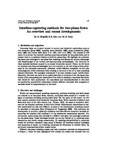
Where D0 is the reference length scale, taken to be the diameter of the bubble. Based on a 10 mm diameter bubble, the Reynolds number and Bond number are 3500 and 140 respectively. For the advection and diffusion terms in the momentum equation (2), third order QUICK scheme is applied. To couple the pressure with the velocity in the incompressible limit, the PISO (pressure implicit with splitting of operators) algorithm is employed, which is performed through two additional neighbor corrections for a better convergence. Pressure staggering option (PRESTO) scheme was used for pressure discretization. The VOF method with the PLIC scheme and CLSVOF method methods are solved explicitly in time and converging at each time step. 4. RESULTS AND DISCUSSION Three different meshes (coarse, medium and fine) with the number of 329000, 729000 and 10470000 elements respectively have been employed to the domain. The numbers of elements across the horizontal and vertical boundaries are 306×1073, 456×1597 and 546×1914. For each of the meshes the number of elements across the bubble is important for the convergence of the interface shape, which for the initial 1cm bubble there are 15800, 52000 and 74646 elements for the coarse, medium and fine mesh. Also, the time step required to solve for the CLSVOF method computations was about 10 times smaller than the VOF method. In Figure 1 the velocity along the centerline and the grid independency of the velocity field for the coarse, medium and fine meshes has been shown before the splitting of the bubble.

Figure 1. Velocity V comparison for 3 meshes

Figure 2 compares the same CLSVOF mesh grid with two other VOF grid meshes. In both cases the thinner line represents the CLSVOF while the darker bold line is the VOF method. Figure 2a shows the coarse CLSVOF and coarse VOF results, and in Figure 2b the same coarse grid for the CLSVOF method with a fine VOF mesh is compared. A finer VOF mesh grid is required to resolve the interface while a coarser mesh grid is sufficient to resolve the interface using the CLSVOF method. This can be seen in Figure 2b where the interface contours lines are very comparable for the Fine VOF and a coarse CLSVOF nesh, but for coarser grids the VOF method tends to over predict the surface tension as it will show an extra stretch as seen in Figure 2a.

Journal of Computational Multiphase Flows

Gholamreza Keshavarzi, Guan Heng Yeoh and Tracie Barber

49

Figure 2. Interface comparison of the Fine VOF mesh with the a) coarse and b) fine CLSVOF mesh at 0.2 s

The shape of the bubble at different stages of the rising progression for both the CLSVOF and VOF method are presented in Figure 3. The black color indicates the CLSVOF method and the red color is the VOF method. The results have been shown for different time steps. The full development of the main bubble rising is also depicted in Figure 4. The deformations of the Level set and VOF are very similar and close to alike for time steps prior to the breakup after skirting. The position and shape of the bubbles are also very comparable along the channel at different heights. For very fine meshes even at the final stages and near top of the column, and after the merging of the smaller bubbles into the large one, the position and velocity of the main large bubble are very similar. Also, The size and shapes of the detached bubbles due to the skirting of the initial circular bubble were shown to be similar for both the CLSVOF method and VOF.

Volume 5 · Number 1 · 2013

50

Comparison of the VOF and CLSVOF Methods in Interface Capturing of a Rising Bubble

Figure 3. Comparison of the VOF and CLSVOF for different time stages

Figure 4. Comparison of the rising bubble for VOF and CLSVOF Journal of Computational Multiphase Flows

Gholamreza Keshavarzi, Guan Heng Yeoh and Tracie Barber

Figure 5. Comparison of fine(black) and Medium(red) VOF mesh grids

51

Figure 6. Comparison of fine(black) and coarse(red) CLSVOF mesh grids

One of the common issues seen with the VOF is with the volume fraction cutoffs and the diffusion accompanied with the interface capturing. This can be seen in Figure 5; while the bubble is rising small bubbles were detached from the main. On the other hand this is less seen with the CLSVOF method. Figures 5 and 6 compare two different mesh grids for both the methods. From the Figure it is understood that the coarse mesh elements tend to over stretch the bubble. Figure 7 is a plot of the velocity contour and velocity vectors. A high velocity field is present underneath the two detached bubbles in the skirting of the initial bubble. This high velocity field along with the reasoning that the smaller bubbles experience a lower drag force and are also in the lower pressure wake region of the large bubble explains the convergence of the smaller bubbles back to the main bubble rising.

Figure 7. Velocity contour-vector at 0.2s VOF Figures 8, 9 and 10 show a plot of the velocity v (velocity in the y direction and pressure along a vertical center line in the channel. The line has been segregated into 200 points to show the velocity Volume 5 · Number 1 · 2013

52

Comparison of the VOF and CLSVOF Methods in Interface Capturing of a Rising Bubble

profile and other detail along the length of the channel. The black line represents the bubble interface and the area in between the black line area is inside the bubble with a volume fraction of 1 for air. The pressure along the same centerline illustrates a trace of lower nonlinear pressure left behind from the large bubble wake and a linear section which is the pressure on top of the bubble. From Figure 8 the results show a very similar velocity profile for the liquid fluid section of the CLSVOF and VOF method, but the CLSVOF shows a higher velocity field along the centerline for the gas fluid in the bubble. Figure 10 shows the effect of mesh sizes on the CLSVOF method on the centerline velocity. It can be seen that the difference seen in the higher velocity on the inside the bubble in CLSVOF becomes less significant for finer meshes, but still from Figure 8 the difference and a higher velocity can be seen for the CLSVOF method compared to the VOF method for the same mesh. From all the Figures it is seen that the main bubble has a top terminal velocity of approximately 0.1m/s, which the bubble reaches that terminal velocity in 0.02 seconds after the release of the bubble. Figure 9 illustrates the velocities for a later time step. At this time step the bubble experiences less deformation and is rising firmly. The velocity is very similar for all positions except for exactly behind the bubble where the wake appears. This Figure also shows that the methods can have significant influence on predicting the flow as well as the interface.

Figure 8. Comparison of the Velocities along the centreline of the channel for VOF and CLSVOF method at 0.1 s

Figure 9. Comparison of the velocity along the centreline of the channel for VOF and Journal of Computational Multiphase Flows

Gholamreza Keshavarzi, Guan Heng Yeoh and Tracie Barber

53

CLSVOF at 0.24 s

Figure 10. Figure 11-CLSVOF velocity along the centreline of the channel at 0.1s

Figure 11. Pressure contour across the bubble a) VOF and b) CLSVOF

Figure 11 helps to understand this which is the plot of pressure across the bubble for both methods at 0.24 second. Since the VOF method does not have a specified exact interface the properties are diffused across the interface. Therefore there is no pressure difference seen across the bubble, conclusively the interface and other properties such as velocity inside the bubble are stabilized. 5. CONCLUSION In the VOF method the exact position of the interface is not known, and the interface is diffused across mesh elements even in very fine meshes. This diffusion is clear in this paper with the pressure plot across the bubble for both methods. The VOF method has no clear indication of the interface and the pressure differences across the interface, and the pressure differences across the interface is not seen. Therefore, this results in stabilizing and damping out small oscillations on the interface in the VOF method, while the CLSVOF shows a much clearer interface and pressure variation across the interface. Finally, although the CLSVOF method has improved the interface capturing significantly and has a much more accurate, less diffusive approach, the CPU calculation required is comparably much more than the VOF. The surface tension is also predicted better in the CLSVOF method, and unlike the VOF method does not require a very fine mesh to capture the details of the interface. The CLSVOF is only affordable for special circumstances and will not Volume 5 · Number 1 · 2013

54

Comparison of the VOF and CLSVOF Methods in Interface Capturing of a Rising Bubble

perform sufficient accuracy after the breakups and converging of the interface, and therefore for 3D cases, implementing the CLSVOF is expensive and requires much higher computation. REFERENCES 1.

Grace, J.R. and D. Harrison, The influence of bubble shape on the rising velocities of large bubbles. Chemical Engineering Science, 1967. 22(10): p. 1337-1347.

2.

Weber, M.E. and D. Bhaga, Fluid drift caused by a rising bubble. Chemical Engineering Science, 1982. 37(1): p. 113-116.

3.

Zheng, Z.L.Y., PIV study of bubble rising behavior. Powder Technology, 2006. 168: p. 10-20.

4.

Gharib, M.W.M., Experimental investigation on the bistable shape states of small air bubbles rising in clean water. 2001.

5.

Collins, R., A simple model of the plane gas bubble in a finite liquid. Journal of Fluid Mechanics, 1965. 22(04): p. 763-771.

6.

Benn, B. and D.W.T.M. Basin., The Drag and shape of air bubbles moving in liquids / by Benjamin Rosenberg1950, Washington, D.C. :: Navy Dept., David W. Taylor Model Basin.

7.

Maneri, C.C. and H.D. Mendelson, The rise velocity of bubbles in tubes and rectangular channels as predicted by wave theory. AIChE Journal, 1968. 14(2): p. 295-300.

8.

Hnat, J.G. and J.D. Buckmaster, Spherical cap bubbles and skirt formation. Physics of Fluids, 1976. 19(2): p. 182-194.

9.

Zhang, Y., Single bubble velocity profile Experiments and Numerical Simulation, 2000, McGill University.

10.

Raymond, F. and J.M. Rosant, A numerical and experimental study of the terminal velocity and shape of bubbles in viscous liquids. Chemical Engineering Science, 2000. 55(5): p. 943-955.

11.

van Wachem, B.G.M. and J.C. Schouten, Experimental validation of 3-D lagrangian VOF model: Bubble shape and rise velocity. AIChE Journal, 2002. 48(12): p. 2744-2753.

12.

Hirt, C.W. and B.D. Nichols, Volume of fluid (VOF) method for the dynamics of free boundaries. Journal of Computational Physics, 1981. 39(1): p. 201-225.

13.

Rudman, M., Volume-Tracking Methods for Interfacial Flow Calculations. International Journal for Numerical Methods in Fluids, 1997. 24(7): p. 671-691.

14.

O, U., Numerical Prediction of Two Fluid Systems with Sharp Interfaces, 1997, University of London: London.

15.

Youngs, D.L., Time-dependent Multi-material Flow with Large Fluid Distortion. Numerical Methods for Fluid Dynamics, Morton, K. W. and Baines, M. J. (Eds.), 1982: p. 273-285.

16.

Sethian, J.A., Theory, algorithms, and applications of level set methods for propagating interfaces. Acta Numerica, 1996. 5: p. 309-395.

17.

Sussman, M. and E.G.Puckett, A Coupled Level Set and Volume-of-Fluid Method for Computing 3D and Axisymmetric Incompressible Two-Phase Flows. Journal of Computational Physics, 2000: p. 301-337.

18.

Smereka, M.S.P., Axisymmetric free boundary problems. Journal of Fluid Mechanics, 1997. 341: p. 269-294.

19.

Son, G. and N.Hur, A Coupled Level Set and Volume-of-Fluid Method for the Buoyancy- Driven Motion of Fluid Particels. Numerical Heat Transfer B, 2002. 42: p. 523-542.

20.

G.Son, Efficient implementation if a coupled Level-set and Volume of Fluid method for three dimensioanl incompressible two phase flows. Numerical Heat Transfer, 2003(43): p. 549–565.

21.

Yeoh, G.H. and T. Barber, Assessment of Interface Capturing Methods in Computational Fluid Dynamics (CFD) Codes — A Case Study. The Journal of Computational Multiphase Flows, 2009. 1(2): p. 201-215.

22.

Atmakidis, T. and E. Y. Kenig, A study on hydrodynamics and mass transfer of moving liquid layers using computation fluid dynamics, in Computer Aided Chemical Engineering, P. Valentin and A. Paul ?erban, Editors. 2007, Elsevier. p. 129-134.

23.

Hayashi, K., R. Kurimoto, and A. Tomiyama, Interface Tracking Simulation of Drops Rising Through Liquids in a Vertical Pipe Using Three Coordinate Systems. The Journal of Computational Multiphase Flows, 2010. 2(1): p. 47-58.

24.

Hernandez-Perez, V., M. Abdulkadir, and B. Azzopardi, Grid Generation Issues in the CFD Modelling of Two-Phase Flow in a Pipe. The Journal of Computational Multiphase Flows, 2011. 3(1): p. 13-26.

25.

Hayashi, K. and A. Tomiyama, Interface Tracking Simulation of Mass Transfer from a Dissolving Bubble. The

Journal of Computational Multiphase Flows

Gholamreza Keshavarzi, Guan Heng Yeoh and Tracie Barber

55

Journal of Computational Multiphase Flows, 2011. 3(4): p. 247-262. 26.

Sussman, M., P. Smereka, and S. Osher, A Level Set Approach for Computing Solutions to Incompressible Two-Phase Flow. Journal of Computational Physics, 1994. 114(1): p. 146-159.

27.

Yeoh, G.H. and J. Tu, Chapter 3 - Solution Methods for Multi-Phase Flows, in Computational Techniques for Multiphase Flows2010, Butterworth-Heinemann: Oxford. p. 95-242.

28.

Brackbill, J.U., D.B. Kothe, and C. Zemach, A continuum method for modeling surface tension. Journal of Computational Physics, 1992. 100(2): p. 335-354.

29.

Puckett, E.G., et al., A High-Order Projection Method for Tracking Fluid Interfaces in Variable Density Incompressible Flows. Journal of Computational Physics, 1997. 130(2): p. 269-282.

Volume 5 · Number 1 · 2013