The object function in turn involves the magnetic flux density. B. In a large subclass of these problems, the flux density may be defined in terms of derivatives of ...
IEEE TRANSACTIONS ON MAGNETICS, VOL. 32, NO 3, MAY 1996
1282
Comparison of Vector Potential and Flux Density Based Object Functions in Magnetic Shape Optimization T. H. Pham', S. Ratnajeevan H. Hoole, Fellow Harvey Mudd College, Department of Engineering Claremont, CA 91711, USA Abstract-In many shape optimization problems, the performance measure is defined in terms of an object function. The object function in turn involves the magnetic flux density B. In a large subclass of these problems, the flux density may be defined in terms of derivatives of the magnetic vector potential A along a tine or, by suitable inspection, simply by the vector potential itself along the line. The two cases are studied in the shape optimization of a pole face. The displacements of the nodes along the pole face are selected as the geometric design parameters. It is shown that where the object function is simply definable in terms of nodal potentials, a very powerful and efficient gradients-based optimization scheme results. Where derivatives of the potential are avoided, it is shown that the object function has a simpler dependence on the geometric parameters of the design because derivatives are strongly influenced by changes in shape. Using a simple nodal potential based object function, smooth geometric contours are obtained without the espense of more elaborate methods of ensuring the smoothness of the optimized geometry.
However, if we held the spacing between the nodes constant as shown in Fig. la, we may work with a line of evaluation as in Fig. la and the flux densities would have a simple dependence only on the nodal vector potential along the line of evaluation, with no direct geometric dependence.
i pl
~
p2
I
p3
j p4
~
p5
a) Line of evaluation running along the elenients edges
I. INTRODUCTION One classical example of electromagnetic device often used to demonstrate and validate electromagnetic optimization methods, is the pole face of a magnetic circuit [I-41. The object is to achieve a uniform flus density distribution B in the air gap. In problems such as these, the object function is defined as a least-square function minimizing the difference between the computed and desired flux densities. Typically, we evaluate the flux density at the sampling points located along
: pl
a line (bolded in Fig. 1). However, because of the
discontinuities in flux density along the element edges, we need a unique definition of the object function, and therefore. we let the line of evaluation run through the triangles (Fig. lb) rather than along element edges (Fig. la). Thus. in the process of optimizing the shape of the object being designed, as the geometric parameters p,, pz, etc. change on account of the shape deformation, the flux density based object function would have a delicate dependence on the vector potentials of all the nodes of triangles through which the line of evaluation passes (with secondary dependence on the other nodes). I Doctoral candidate at the Laboratoire Electrotechnique de Grenoble, Ecole Nationate Superieure dhgenieurs-Electriciens de Grenoble, TNPG. France. Now with Magsoft Corporation, 1223 Peoples Avenue, Troy, N Y 12180, USA Manuscript received: July 10, 1995.
:
p2
:
p3
I p4
:
p5
hj Line o f evaluation running through the triangles
Fig. 1. Line of evaluation for flux density dependent object function
The gradients with respect to the geometric design parameters become much simpler. and it is shown in this paper, much better convergence characteristics are realized. It is also shown in this paper that as a result of the simpler dependence of the objective function, gradual changes of the geometry result, as optimization iterations occur, and as a consequence, a smooth geometric contour is obtained. As a result of jagged geometric contours, three techniques proposed to overcome this problem and published [1-3] need to be made recourse to less often. The first technique [ 11 uses
0018-9464/96$05.00 0 1996 IEEE
1283
"manual smoothing" to render the results useful. The second technique 121 is based on a structural mapping technique to deform uniformly the finite element mesh. The third technique adds linear constraints on the gradient of the design parameters to impose the regularity constraints along the pole face [3]. In contrast, our object is to develop an economical and simpler method for shape optimization of electromagnetic devices. It relies only on electromagnetic finite element analysis, a magnetic vector potential based object function, and gradient optimization methods. 11. OPTIMIZATION SOLUTION OF THEPOLE FACEB Y FINITE ELEMENT ANALYSIS In two dimensional finite element field computation in electromagnetic systems, the solution region comprising the device and some of its neighborhood is discretized into elements and the magnetic vector potential A, reduced to its scalar component A perpendicular to the plane of analysis, is computed from the matrix equation [5]:
where Ip] and {Q} are respectively tlie global Dirichlet matrix and the global source current density vector. The left and right boundaries are the lines of symmetry and tlie geometry being optimized is as described in 12-31, In this work, unlike what has been reported in the literature [2-31, all the nodes along the pole face are chosen as design parameters {p} = {pl, p2. .., p,}.
matrices. Thus, we can obtain
3
through the
@I
differentiation of (1) and the solution of: (4) Where the line of evaluation runs as in Fig. Ib through triangles, the gradient can be computed using the interpolation form of Ak in the element e where the sampling point k is located.
B. Flux density based object function The flus density based object function Fb(B) is defined as a least square function that describes the difference of the ynumerically computed by component of the flus density, the finite element method. from the desired values Bopck(in the pole face model. Bop,.kis constant and equal to 1 along the line of sampling points) at the defined sampling points k in the air gap (Fig. 2 ) .
(7) A . Magnetic vector potential based object function The magnetic vector potential based objective function Fa(A) is defined as a least square form of the difference of the scalar magnetic potential A, calculated at the sampling points from their desired values Aopt,k(Fig. 2).
To apply the gradient based optimization methods, the gradient of F, with respect to each design parameter pi of { p} is required:
2
Fa = E k ["-1 Aopt,k ) Because A is zero at the right-most sampling point on the Dirichlet boundary, and because the desired constant flus density gives us the slope of A as we move along the line of evaluation, the desired vector potential is known to be as in Fig. 7. To apply gradient optimization methods, the gradient of Fa with respect to each design parameter p, of {p} is required:
The gradients can be computed without a second field solution [2] by using the differentiability of the finite element
The term
aB,,k can be calculated from the differentiation of 0
1
the following equation:
In the element e where the sampling point k is located, A(s,,y,) is approximated by the nodal magnetic potential values {A}, and the first order interpolation functions { C L ( Sk. y h )} = {a} + { b}' SI. + {C}' y I, :
1284
The gradient of By,kis then:
{e}
Likewise the magnetic vector potential based object function case,
is obtained.through the solution of (4). When
e
the field solution of (1) is available and with the Choleski decomposition of PI, the solution of (4) is reduced to the assembly of the right hand side of (4), and forward and backward substitutions using the already decomposed coefficient matrix. 111. OPTIMIZATION RESULTS
A. Magnetic shape optiinizatioii bench niark The bench mark of optimizing the pole face of a magnetic circuit (Fig. 2) is used. The object is to achieve a uniform flux density distribution By in the air gap. There is a large leakage flux at the left edge of the pole face. The influence of this leakage flux requires significant corrections i n the shape of the pole face close to the left edge in order to achieve the desired constant flux density in the air gap. All the nodal coordinates along the pole face are selected as design parameters. The optimization was performed using a conjugate gradient method.
Fig. 3. Optiiiiuin shape ofthe pole face using Fb
Although the object function F, decreases from 0.65 for the initial shape to 0.0031 (Fig. 4) at the optimal shape and the object (BcalcB)is achieved within a tolerance of 2% as depicted in Fig. 8, the optimal pole face has a jagged and impracticable shape.
Flus Density based Fb Object Functions Line of
Iron
0
sampling points
2
4
6
8
1 0 1 2 1 4
I
I
\1/ III
Pole face at initial geometry
Air
---_._-..-
0.01
Coil \
.
Pole face at optimum grometq
I
Iron
Fig. 2. Shape optimization bench mark of a magnetic circuit pole face
B. Optimization results: frux density bnsed object fiiiiction The optimum shape which is given with the corresponding equipotential lines of the magnetic vector potential A in Fig. 3 is obtained after 14 optimization iterations.
-
-
0.001 Number of Iterations Fig. 4. Flux density bnsed objective fiinction
C. Optimizntion results: ningnetic vector based object Jinctioi? A smooth pole face shape is obtained for the magnetic vector potential based object function F, (2) after only 5 optimization iterations (Fig. 5 ) . The value of Fa decreases from 0.85 at the initial geometry to 0.0002 at the optimum geometry (Fig. 6). The object for the vector potential is achieved within a tolerance of 1% (Fig. 7).
1285
Magnetic vector potentials along the sampling points line 4
3.5
3 2.5
A 2 1.5 1
0.5
0 6
6. 4
6. 8
1. 7. 2
8
6
8. 4
8. 8
9. 2
9. 6
10
X coordinate of the sampling points Fig. 7. Magnetic vector potentials along the line of sampling points
By at sampling points Fig. 5 . Optimum shape of die pole face using Fa
1.1
Magnetic Vector Potential based Object Function Fa
0
2
1
3
4
-0-BcalcA Bopt -ABcalcB
-
-
1.05 5
\
0.1
k
Fa
\
0.01
--
I
x
\
0.001
- - *
6
V
0.0001
7. 2
7. 6
8
8. 4
8. 8
9. 2
9. 6
10
Fip 8. Flux densities along the lirie o f sarnyling points
Number of Iterations Fig. 6. Magnetic vector potential based object function Fa
ii has been shown that it is desirable to use ~ i i ( c v potential based object functions rather than flux ilensrty based ones. Convergence is faster, smoother geometries, and the computation is simpler. In the case, where an optimum potential profile is available (i.e. the shape optimization of inductor coil in an induction heating process to wtiyPJ ;i clc\iic.d temperature pi ofilc j, this method is suci\\Jii!i) .try I1e(I [61.
6. 8
X coordinate of the sampling points
J
The equivalent object for the flux density (in Fig. 8 BcalcA)is achieved also within the 2% error margin everywhere except in the regit>r:at the left edge of the pole face, where thcre is a 7% crror
6. 4
REFERENCI[ 11
[21
!i1
[5] [6]
?
0. Pironneau, Optimal Shupe Design for Ellipric, Systems, Spring-Verlag, New York, 1984. K. Weber and S . Ratnajeevan H. Hoole, "A Structural Mapping Technique for Geometric Parametrization in the Synthesis of Magnetic Devices," Int. J. Num. Meth. Eng., Vol. 33, pp. 2145-2179, 1992. S. Subramaniam, A. A. Arkadan, S . Ratnajeevan H. Hoole, "Optimization of a Magnetic Pole Face Using Linear Constraints to Avoid Jagged Contours," ZEEE Trans. On Mugn., Vol. 30, No. 5, September 1994. S . Ratnajeevan H. Hoole, Finite Elements, Electromagnetics, and Designs, Elsevier, Amsterdam, 1995. S. R. H. Hoole, Computer-Aided Analysis and Design of Electromagnetic Devices, Elsevier; New York, 1989. T. H. Pham and S . R. H. Hoole, "Unconstrained Optimization of Coupled Magneto-Thermal Problems Pole Face," ZEEE Trans. On Mugn., Vol. 3 I , No. 3, May 1995.