Dynamical localization, measurements and quantum computing

Dynamical localization, measurements and quantum computing M. Terraneo and D. L. Shepelyansky Laboratoire de Physique Th´eorique, UMR 5152 du CNRS, Univ. Paul Sabatier, 31062 Toulouse Cedex 4, France (Dated: September 26, 2003) We study numerically the effects of measurements on dynamical localization in the kicked rotator model simulated on a quantum computer. Contrary to the previous studies, which showed that measurements induce a diffusive probability spreading, our results demonstrate that localization can be preserved for repeated single-qubit measurements. We detect a transition from a localized to a delocalized phase, depending on the system parameters and on the choice of the measured qubit.

arXiv:quant-ph/0309192v1 26 Sep 2003

PACS numbers: 05.45.Mt, 03.65.Ta, 03.67.Lx, 02.70.Uu

In 1979 the dynamical localization of quantum chaos was discovered in numerical simulations of the kicked rotator model [1]. It was found that the unbounded classical diffusion typical of chaotic dynamics is suppressed by quantum interference effects [1, 2]. This interesting phenomenon found its explanation on the basis of an analogy with the Anderson localization in disordered lattices [3] (see also [4]). Manifestations of dynamical localization appear in various physical systems. Its first experimental observation was obtained with hydrogen and Rydberg atoms in a microwave field [5]. Recently, a significant technological progress in manipulating cold atoms by laser fields allowed to build up experimentally the kicked rotator model and to study dynamical localization in real systems in great detail [6, 7, 8]. Since localization appears due to quantum interference it is natural to expect that it is rather fragile and sensitive to noise and interactions with the environment. Indeed, in theoretical and experimental studies it was shown that even a small amount of noise destroys coherence and localization [7, 8, 9]. Measurements represent another type of coupling to the environment [10], and it is of fundamental importance to understand their effects on dynamical localization. Theoretical and numerical studies show that measurements destroy localization and induce a diffusive energy growth like in the case of a noisy environment [11, 12, 13]. For weak continuous measurements, discussed in [11], the rate of this growth can be much smaller than the diffusion rate induced by classical chaos. However in the limit of strong coupling to the measurement device the quantum diffusion rate becomes close to its classical value. A similar situation takes place in the case of projective measurements, considered in [12, 13]. The interest in measurement procedures enormously grew up in the last years due to progress in quantum information processing [14]. Indeed, the extraction of information from a quantum computation is always reduced to a final measurement of the quantum register. Various experimental implementations were discussed for the realization of the readout procedure in quantum optics systems [15, 16] and solid state devices [17, 18, 19, 20]. Moreover it has been shown that a quantum computation

can be performed completely by a sequence of measurements applied to an initially entangled state [21]. At the same time, measurements represent an important part of various quantum algorithms, including the famous Shor algorithm for the factorization of integers [22]. Therefore it is important to investigate the effects of measurements on quantum computers operating nontrivial algorithms. An interesting example is the quantum algorithm proposed in [23] which allows to simulate the evolution of the kicked rotator on a quantum computer. This algorithm essentially uses the Quantum Fourier Transform (QFT) and controlled phase gates. It realizes one map iteration in a polynomial number of quantum gates (O(n3q )) for a wave vector of size N = 2nq . Here nq is the number of qubits (two-level quantum systems) onto which a kicked rotator wave function is encoded. For moderate kick amplitudes, this algorithm can be replaced by an approximate one which uses all the qubits in an optimal way and performs one map iteration in O(n2q ) elementary gates [24]. In this form the algorithm can simulate complex dynamics, e.g. the Anderson transition, with only a few (∼ 7) qubits. This makes it accessible for possible future realization on NMR based quantum computers. Indeed, all the elements of the algorithm have already been implemented on NMR quantum computers [25, 26]. Therefore it represents an interesting testing ground for the investigation of the measurement effects on dynamical localization in a quantum computation. The quantum evolution of the kicked rotator is deˆ acting on the wave scribed by the unitary operator U function ψ [4]: ˆ

2

ˆψ = U ˆk · U ˆT ψ = e−ik cos θ e−iT nˆ ψ=U

/2

ψ.

(1)

ˆk Here ψ is the wave function after one map iteration, U represents the effects of the kick in the phase represenˆT describes the free rotation in the momentation and U tum basis n with n ˆ = −i∂/∂θ (we use units with ~ = 1). The dimensionless parameters k, T determine the kick strength and the rotation phases, so that the classical limit corresponds to k → ∞, T → 0 with the chaos parameter K = kT constant. Here we study the regime of

2

ˆk · U ˆT · ρˆ · U ˆ† · U ˆ † · P0 (m) + ˆ = P0 (m) · U ρ T k † ˆ† ˆ ˆ ˆ P1 (m) · Uk · UT · ρˆ · U · U · P1 (m) T

k

(2)

ˆ is the density matrix after one map iteration with Here, ρ measurement. The direct simulation of this equation is quite costly, since N 2 components should be iterated. To avoid this difficulty we used the method of quantum trajectories [27]. In this method for one quantum trajectory the wave function ψ evolves according to (1); after each map iteration ψ in the momentum representation is pro-

t 10 10

3

10

2

10

1

10

0

0

10

1

10

2

10

3

10

4

10

5

10

6

10

5

10

4

2



ξ

dynamical localization corresponding to l ≪ N , where l ≈ k 2 /2 is the localization length [4]. The quantum algorithm simulating the evolution (1) operates as described in [23, 24]. The wave function ψ in the momentum representation with N = 2nq levels is encoded on a quantum computer with nq qubits. In this way n = −N/2 + j where the index j = 0, . . . , N − 1 is written in the binary representation as j = (a1 , a2 , . . . , am , . . . , anq ), with am = 0 or 1. As the initial state we choose the momentum eigenstate at n = n0 = 0, which can be efficiently prepared from the ground state. Then, as described in [23] the rotaˆT is performed in O(n2q ) controlled-phase gates. tion U After that the QFT transforms the wave function to θrepresentation in O(n2q ) quantum elementary gates (see ˆk is realized in O(n3q ) gates [14]). The kick operator U with the help of an additional register [23], or, for moderate k values, it can be approximately implemented in O(nq ) gates without any ancilla, following [24]. Finally, ψ is transformed back to the momentum basis by the inverse QFT. Here we assume that the gates are implemented without errors, keeping the analysis of imperfection effects for further studies. To study the effects of measurements on the dynamics given by the above algorithm we assume that after each map iteration (1) a projective measurement of a chosen qubit m is performed. The measurement can be represented as the action of two projection operators P0 (m) and P1 (m) giving for am an outcome 0 or 1 with the probability ||P0 (m)ψ||2 or ||P1 (m)ψ||2 , respectively. The measurement projects the wave function onto one of two subspaces of the total Hilbert space, corresponding to momentum states labeled by the indexes j = (a1 , a2 , . . . , am , . . . , anq ) with fixed am = 0 or am = 1. Each subspace is composed of N/2 states, given by the direct sum of 2m−1 cells of L = 2nq −m consecutive momentum states. For example, for m = 1 the most significant qubit is measured and ψ is projected onto momentum states with −N/2 ≤ n < 0 (a1 = 0) or 0 ≤ n ≤ N/2 − 1 (a1 = 1); for m = nq the least significant qubit is measured and ψ is projected onto even and odd momentum states. Such a measurement is the most natural one for the quantum computation process. Thus, the evolution with measurements is given by the following equation for the density matrix ρˆ

10

0

10

1

10

2

10

3

10

4

10

5

10

3

10

2

10

1

10

0

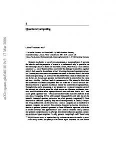
t FIG. 1: (Color on line) Dependence of the second moment hn2 i on time t. Here T = 2, k = 2 and color marks the value of nq . The upper group of curves corresponds to the measurements of the least significant qubit m = nq for nq = 12 (blue), 11 (violet), 10 (red) and 9 (black), from top to bottom. In the lower group one of most significant qubits is measured with m = nq − 8 for nq = 12 (black) and 9 (yellow) (data for nq = 10, 11 give same superimposed curves and are not shown). The lowest green fluctuating curve is the evolution without measurements. The dashed line shows the diffusive growth hn2 i ∼ t. The inset shows the dependence of the IPR ξ on t (colors are as in the √ main plot, the dashed line shows the diffusive growth ξ ∼ t).

jected on the subspaces with am = 0 or 1 according to the probability ||P0 (m)ψ||2 or ||P1 (m)ψ||2 , respectively. After the renormalization, this gives the wave function ψn in the momentum basis. The density matrix and the expectation values of observables are then obtained by averaging over M quantum trajectories. To characterize the quantum evolution with measurements we compute the following quantities: the probability distribution ρnn ≈ h|ψn |2 i, obtained by averaging |ψn |2 over M quantum trajectories; the second moment of thePprobability distribution, given by hˆ n2 i = 2 2 2 Inverse Participation RaT r(ˆ n ρˆ) ≈ n nPh|ψn | i; the P tio (IPR) ξ = 1/ n ρ2nn ≈ 1/ n |h|ψn |2 i|2 which determines the number of states on which the average probability is distributed. Within statistical fluctuations these quantities remain unchanged for a variation of M from 20 to 500 and we represent them for M = 50. The dependence of hˆ n2 i and ξ on the number of map iterations t is displayed in Fig.1 for different nq and m. The probability distribution h|ψn |2 i for nq = 10 is shown in Fig.2. These data clearly show that the measurement of the least significant qubit completely destroys localization generating a diffusive behavior. Indeed, the second moment hˆ n2 i and the IPR ξ grow diffusively (see Fig.1) up to spread of the probability over the whole computa-

3 0

10

2500



200 −5

10

2000

100

−5

10 −10

10

−15

−15

10

−25

−500

0

5

1500

10 500

10

15

20

0

k



|ψn|

2

10

1000 −20

10

500

−25

10

−500

−250

0

250

500

n

FIG. 2: (Color on line) Probability distribution for k = 2, T = 2, nq = 10 at t = 5 × 105 . Measurements are done for m = nq − 8 that preserves localization (black curve) and for m = nq that leads to extended distribution (red curve). The distribution for evolution without measurements is shown by green/gray curve. Data are averaged over 50 quantum trajectories. The inset shows |ψn |2 for a single quantum trajectory (same colors).

tional basis, as shown in Fig.2. The extended distribution h|ψn |2 i is formed by a superposition of probabilities |ψn |2 generated by single quantum trajectories (see Fig. 2 inset, which shows that each |ψn |2 is relatively narrow). On the contrary, the measurement of one of the most significant qubits does not destroy localization, as clearly illustrated in Figs.1, 2. This striking result is very different from the previous studies [11, 12, 13] where localization was always destroyed by measurements. To understand the origin of this behavior we investigate the dependence of the averaged IPR hξi on the kick amplitude k for different number of qubits nq (see Fig.3). For k ≤ kc ≈ 6 the IPR is independent of nq , corresponding to a localized regime. On the contrary, for k > kc the IPR starts to grow with the system size N = 2nq , indicating a transition to a delocalized phase. We explain the appearance of this transition in the following way. The measurement process determines the cell size L = 2nq −m inside which the coherence of quantum dynamics is preserved. If the unperturbed localization length l is much smaller than the cell size, then measurements do not destroy dynamical localization. While, if l ≫ L, the wave function propagates over different cells, measurements destroys quantum coherence between nearby cells and this leads to a diffusive propagation over the computational basis. According to our data the delocalization transition takes place when ξ0 ≈ 2l ≈ k 2 ≈ L/5

(3)

where ξ0 is the IPR for the dynamics without measurements (see the inset in Fig.3). This relation shows that the transition can be obtained by tuning k at fixed nq − m or by an appropriate variation of m at fixed k.

0

0

5

10

15

20

k FIG. 3: Dependence of the averaged IPR hξi on k for measurements of one of the most significant qubits m = nq − 8, for nq = 9 (squares); 10 (diamonds); 11 (triangles); 12 (stars). IPR values are averaged over 1000 kicks around t = 5 × 105 ; T = 2. The inset shows the same dependence in the absence of measurements.

Our numerical data confirm this estimate. Indeed, for m = nq − 9 we obtain that k = 10 is localized, while at k = 12 delocalization takes place (data not shown). It is interesting to note that the oscillations of hξi in Fig.3 are correlated with the oscillations of ξ0 , thus confirming that the delocalization border is determined by the unperturbed localization length l (these oscillations are produced by dynamical correlations which affect the classical/quantum diffusion rate related to the localization length l as discussed in [28]). To study the quantum dynamics at larger time scales we use the random quantum phase method proposed in [12]. It is based on the fact that after a projection on a given quantum state induced by a measurement the quantum phase is not defined. Therefore one can assume that states associated to different outcomes of the measurement procedure have a random relative quantum phase. Thus, after a measurement of the m-th qubit the state |φi is replaced by eiβ0 P0 (m)|φi + eiβ1 P1 (m)|φi, where the phases β0,1 are random. This approach allows to reduce significantly the computational cost of the simulation, since it effectively integrates the dynamics over many quantum trajectories. The comparison of the two computational methods is presented in Fig.4, for diffusive, localized and critical regimes. Both methods give consistent results for hn2 i (Fig.4) and the IPR (data not shown). With the random quantum phase method we can follow the evolution for very large times (up to t = 107 ) at which localization is still preserved (see Fig.4 b). This computational method allows also to understand in a better way why localization is not destroyed by measurements. Indeed, the effects of random phase fluctuations β0,1 appear only at the cell boundaries. Hence, for L ≫ l they do not

4 t

2



2



10 10

5

10

3

10

1

10

3

10

2

10

1

10

0

1

10

3

10

5

a)

b)

10

1

10

3

10

5

10

7

t FIG. 4: (Color on line) Time dependence of the second moment hn2 i of the quantum distribution obtained by the computation with quantum trajectories (blue and black curves) and with the random quantum phase method (yellow/gray and green/gray curves); T = 2, nq = 10. Panel a) shows diffusive regime for k = 6 (upper blue and yellow curves) and k = 2 (lower black and green curves), for m = nq ; the straight line gives the diffusive law hn2 i ∼ t. Panel b) shows a localized regime for k = 2 (lower curves) and a near critical case for k = 6 (upper curves), for m = 2; the straight line shows anomalous diffusion hn2 i ∼ t0.2 , colors are as in panel a).

affect the momentum states located on a distance larger than l from edges and localization is preserved [29]. We think that the same mechanism qualitatively explains the results obtained in [30] where it was found that measurements of a 1/2-spin detector coupled to the kicked rotator do not destroy localization. In this case the effective cell size L is the total number of rotator momentum states and thus localization is preserved since l ≪ L. In conclusion, we studied the effects of measurements on dynamical localization in a quantum algorithm simulating the kicked rotator. Contrary to the common lore the localization is not always destroyed by measurements, and a transition from localized to diffusive dynamics takes place when system parameters are varied. The authors acknowledge useful discussion with S.Bettelli, B.Georgeot. We thank CalMiP in Toulouse and IDRIS in Orsay for access to their supercomputers. This work was supported in part by the EC projects RTN QTRANS and IST-FET EDIQIP and the NSA and ARDA under ARO contract No. DAAD19-01-1-0553.

[1] G. Casati, B. V. Chirikov, F. M. Izrailev and J. Ford, Lecture Notes in Physics, 93, 334 (1979). [2] B.V.Chirkov, F.M.Izrailev and D.L.Shepelyansky, Sov. Scient. Rev. (Gordon & Bridge) 2C, 209 (1981).

[3] S. Fishman, D. R. Grampel and R. E. Prange, Phys. Rev. Lett. 49, 509 (1982). [4] F. M. Izrailev, Phys. Rep. 196, 299 (1990); S. Fishman, in Quantum Chaos, Proceedings of the International School of Physics “E. Fermi”, Course CXIX edited by G. Casati, I. Guarneri and U. Smilansky (Elsevier, Amsterdam, 1992). [5] See review by P. M. Koch and K. A. H. van Leeuwen, Phys. Rep. 255, 289 (1995). [6] F.L.Moore, J.C.Robinson, C.F.Bharucha, B.Sundaram and M.G.Raizen, Phys. Rev. Lett. 75, 4598 (1995). [7] H.Ammann, R.Gray, I.Shvarchuck and N.Christensen, Phys. Rev. Lett. 80, 4111 (1998). [8] M. K. Oberthaler, R. M. Godun, M. B. d’Arcy, G. S. Summy, and K. Burnett, Phys. Rev. Lett. 83, 4447 (1999) [9] D.L.Shepelyansky, Physica D 8, 208 (1983); E. Ott, T. M. Antonsen, Jr., and J. D. Hanson, Phys. Rev. Lett. 53, 2187 (1984). [10] W.H.Zurek, Rev. Mod. Phys. 75, 715 (2003). [11] T. Dittrich and R. Graham, Europhys. Lett. 11, 589, (1990); Phys. Rev. A 42, 4647 (1990). [12] B. Kaulakys and V. Gontis, Phys. Rev. A 56, 1131 (1997). [13] P. Facchi, S. Pascazio and A. Scardicchio, Phys. Rev. Lett. 83, 61 (1999). [14] M. A. Nielsen and I. L. Chuang, Quantum Computation and Quantum Information (Cambridge University Press, Cambridge, 2000). [15] J. I. Cirac and P. Zoller, Phys. Rev. Lett. 74, 4091 (1995) [16] H.M.Wiseman and G.J.Milburn, Phys. Rev. A 47, 642, (1993); H.M.Wiseman, Phys. Rev. Lett. 75, 4587 (1995). [17] S.A. Gurvitz, Phys. Rev. B 56, 15215 (1997). [18] A.N. Korotkov, Phys. Rev. B 60, 5737 (1999). [19] D.V. Averin, Phys. Rev. Lett. 88, 207901 (2002). [20] M.H. Devoret, and R.J. Schoelkopf, Nature 406, 1039 (2000). [21] R. Raussendorf and H. J. Briegel, Phys. Rev. Lett. 86, 5188 (2001). [22] P. W. Shor, in Proceedings of the 35th Annual Symposium Foundations of Computer Science, edited by S. Goldwasser, (IEEE Computer Society, Los Alamitos, CA, 1994), p.124. [23] B. Georgeot and D. L. Shepelyansky, Phys. Rev. Lett. 86, 2890 (2001). [24] A. Pomeransky and D. L. Shepelyansky, quant-ph/0306203. [25] L. M. K. Vandersypen, M. Steffen, G. Breyta, C. S. Yannoni, M. H. Sherwood, I. L. Chuang, Nature 414, 883 (2001). [26] Y. S. Weinstein, S. Lloyd, J. Emerson, and D. G. Cory Phys. Rev. Lett. 89, 157902 (2002) [27] H.J. Carmichael, An Open Systems Approach to Quantum Optics, (Springer, Berlin, 1993); T.A. Brun, Am. J. Phys. 70, 719 (2002). [28] D. L. Shepelyansky, Phys. Rev. Lett. 56, 677 (1986). [29] We cannot exclude that this noise may produce hardly observable unlimited diffusion with a rate ∝ exp(−2L/l). [30] S.Sarkar and J.S. Satchell, Europhys. Lett. 4, 133 (1987).