Compression of multi channel audio at low bit rates ...

2005:134 CIV

MA S T ER’S T H E SI S

Compression of Multi Channel Audio at Low Bit Rates Using the AMR-WB+ Codec

LARS ABRAHAMSSON

MASTER OF SCIENCE PROGRAMME Technical Physics Luleå University of Technology Department of Mathematics

2005:134 CIV • ISSN: 1402 - 1617 • ISRN: LTU - EX - - 05/134 - - SE

Compression of multi channel audio at low bit rates using the AMR-WB+ codec

Lars Abrahamsson

Abstract The purpose of this thesis work done at Ericsson Research in Lule˚ a was to investigate the possibilities of encoding 5.1 surround sound for low bit rates using the AMR-WB+ audio encoding technique. In the first phase of the work, investigations of the inter-channel dependencies were carried out, and the main tool used was Matlab. Several efforts were made aiming to reduce the total energy of the signal. This was done by decorrelating the sound channels using ordinary linear predictors. Decorrelation attempts were performed in the time domain as well as in the frequency domain. After decorrelating the channels, each channel was encoded in an individual bit rate using the mono mode of AMRWB+ with bit rates proportional to the relative energy content. However, listening tests combined with studies of the energy reduction achieved by decorrelations indicated that, for a given bit rate, there is in general no advantage decorrelating the signal compared to not doing so. The second phase of the thesis work mainly consisted of modifying the existent C code of the AMR-WB+ mono coder in order to suit it for 5.1 sound encoding and decoding. The goal was “the simplest possible”, an encoder that encoded each unmodified sound channel individually, distributing the bit rates over the channels aiming to keep the sums of the bit rates over the channels approximately constant over time. Opposed to the five “normal” sound channels, the encoding of the LFE (Low Frequency Element) was done in a specific way making use of this, compared to the other channels, somewhat constrained signal. Furthermore, the method of encoding high frequency sounds of AMR-WB+, the BWE (BandWidth Extension), needed to be modified at some extent. Finally, the third phase consisted mainly of evaluation of the product made and of making comparisons to competing low bit rate multi channel coders.

i

Sammanfattning Syftet med detta examensarbete som gjordes p˚ a Ericsson Research i Lule˚ a var att utreda m¨ ojligheterna att koda 5.1-kanalsljud f¨ or l˚ aga bittakter med hj¨ alp av ljudkodaren AMR-WB+. I arbetets f¨ orsta fas utreddes ljudkanalernas ¨ omsesidiga beroenden, och huvudverktyget var Matlab. Flera olika insatser gjordes i syfte att f¨ ors¨ oka reducera signalens totala energi. Dessa f¨ ors¨ ok innebar reduktion av korrelationerna ljudkanalerna emellan. Korrelationernas reduktioner ˚ astadkoms med hj¨ alp av vanliga linj¨ ara prediktorer. Korrelationsreduceringsf¨ ors¨ ok utf¨ ordes s˚ av¨ al i tidsdom¨ anen som i frekvensdom¨ anen. Efter att ha reducerat korrelationerna kanalerna emellan kodades varje kanal i en individuell bittakt genom att anv¨ anda AMR-WB+:s monol¨ age. Varje kanals bittakt var proportionellt relaterad till kanalens relativa energiinneh˚ all. Emellertid visade lyssningstest i kombination med studier av den av korrelationsminskningen uppn˚ adda energireduktionen att, f¨ or en given bittakt, ger det i allm¨ anhet ingen vinst att reducera korrelationerna i signalen i j¨ amf¨ orelse med att inte g¨ ora det. Arbetets andra fas bestod till st¨ orsta delen av att modifiera befintlig C-kod fr˚ an AMR-WB+:s monokodare. Syftet med modifikationerna var att anpassa kodaren till att kunna koda och avkoda 5.1 flerkanalojliga”, det vill s¨ aga en kodare som sljud. M˚ alet sattes till ”det enklast m¨ kodade varje or¨ ord ljudkanal individuellt, och f¨ ordelade bittakterna ¨ over kanalerna med avsikten att h˚ alla summan av bittakter, ¨ over kanalerna, approximativt konstant i tiden. Till skillnad fr˚ an de fem ”normala” ljudkanalerna, kodas l˚ agfrekvenselementet p˚ a ett speciellt s¨ att f¨ or att dra nytta av denna, i j¨ amf¨ orelse med de andra ljudkanalerna, n˚ agot begr¨ ansade kanal. Vidare beh¨ ovde BWE:n (BandWidth Extension), metoden vilken AMR-WB+ anv¨ ander f¨ or att koda h¨ ogfrekvensljud, modifieras i viss utstr¨ ackning. Slutligen bestod den tredje fasen huvudsakligen av utv¨ ardering av den framtagna kodaren samt att g¨ ora j¨ amf¨ orelser med konkurrerande l˚ agbittakts kodare av flerkanalsljud.

ii

Acknowledgements My supervisor at Ericsson Research has been Ingemar Johansson, who has been of great help thanks to his experience, helpfulness, easy manner and skill. The help of his spans of course all the work done, but the most critical part has been the C programming where his help has been a necessity. My experience of C programming was before this thesis work close to nonexistent. I have had a shorter optional C++ course at upper secondary technical school only that is all. Except Ingemar, people supporting me in writing this thesis are Tomas Frankilla at Ericsson Research – proof reading, and my sister ˚ Asa – giving me support regarding the English language. Technical aid concerning Scientific WorkPlace is received from Johan Dasht, PhD student at the mathematics department of Lule˚ a University of Technology. Furthermore, thanks go to Amelia Schulteis, a German acquaintance I met at CERN last summer, for the help of managing the X-Fig/Win-Fig and Pstoedit picture editing and conversion programs. I would also like to thank the rest of the staff at Ericsson that I have got help and inspiration from, the computer technicians at TietoEnator as well as my examiner at the university – Thomas Gunnarsson. Thomas Gunnarsson is prefect at the department of mathematics at Lule˚ a University of Technology.

iii

Contents Contents

iv

List of Figures

vi

List of Tables

ix

1 Introduction 1.1 Background . 1.2 Applications . 1.3 Teaser . . . . 1.4 Outline of the

. . . . . . . . . . . . Thesis

. . . .

. . . .

. . . .

. . . .

. . . .

. . . .

. . . .

. . . .

. . . .

. . . .

. . . .

. . . .

. . . .

. . . .

. . . .

. . . .

. . . .

. . . .

. . . .

. . . .

. . . .

. . . .

. . . .

. . . .

. . . .

2 The Problem

1 1 1 1 2 3

3 Brief Description of the mono coder of AMR-WB+ 3.1 Time Separation . . . . . . . . . . . . . . . . . . . . . 3.2 Pre-emphasis and LP Filtering . . . . . . . . . . . . . 3.3 Immitance Spectral Frequency (ISF) . . . . . . . . . . 3.4 The ACELP Coder . . . . . . . . . . . . . . . . . . . . 3.5 The TCX Coders . . . . . . . . . . . . . . . . . . . . . 3.6 BandWidth Extension (BWE) . . . . . . . . . . . . . 3.7 Internal Sample Frequency (ISF) modes . . . . . . . . 3.8 Available Bit Rates of the Coder . . . . . . . . . . . .

. . . . . . . .

. . . . . . . .

. . . . . . . .

. . . . . . . .

. . . . . . . .

. . . . . . . .

4 4 5 6 7 9 13 15 15

4 Feasibility Study 16 4.1 Background Information . . . . . . . . . . . . . . . . . . . . . . . 16 4.2 The Matlab Simulations . . . . . . . . . . . . . . . . . . . . . . . 17 4.2.1 Introduction . . . . . . . . . . . . . . . . . . . . . . . . . 17 4.2.2 Band Splitting in the Time Domain . . . . . . . . . . . . 19 4.2.3 Recombination of the Split Signal . . . . . . . . . . . . . 22 4.2.4 Creation of Sum and Difference Channels . . . . . . . . . 22 4.2.5 Different Dependency Chains . . . . . . . . . . . . . . . . 24 4.2.6 Time Windowing . . . . . . . . . . . . . . . . . . . . . . . 24 4.2.7 Time Domain Decorrelation . . . . . . . . . . . . . . . . . 26 4.2.8 Time Domain Reconstruction . . . . . . . . . . . . . . . . 29 4.2.9 Two Smaller Dependency Chains . . . . . . . . . . . . . . 31 4.2.10 Additional Ideas Regarding the Decorrelation Efforts Made in the Time Domain . . . . . . . . . . . . . . . . . . . . . 33 4.2.11 Frequency Domain Decorrelation . . . . . . . . . . . . . . 34 4.2.12 Examples of FFT Domain Decorrelation . . . . . . . . . . 38 4.2.13 Bit Rate Allocation and Reference Channel Puzzles . . . 43 4.2.14 FFT Domain Reconstruction . . . . . . . . . . . . . . . . 44 4.2.15 Experiments Using the HF Part of the Front Channels in the Rear Channels as Well . . . . . . . . . . . . . . . . . . 44 iv

4.3

4.4 4.5

4.2.16 FFT Domain Results . . . . . . . . . . . . . . . . . . . . . Modifications of AMR-WB+ needed to be made . . . . . . . . . 4.3.1 Introduction . . . . . . . . . . . . . . . . . . . . . . . . . 4.3.2 The Bass Channel, Also Known as the Low Frequency Element (LFE) . . . . . . . . . . . . . . . . . . . . . . . . 4.3.3 The Addition of Six Extra Low Bit Rate (TCX) Modes . 4.3.4 BandWidth Extension (BWE) . . . . . . . . . . . . . . . 4.3.5 The Noise-fill Feature of the Decoder . . . . . . . . . . . . Bit Rate Allocation . . . . . . . . . . . . . . . . . . . . . . . . . . Conclusions . . . . . . . . . . . . . . . . . . . . . . . . . . . . . .

46 46 46 47 48 49 49 53 59

5 Comparisons

60

6 Conclusions

61

7 Discussions 7.1 Making Use of the Existence of “Cheap” Surround . . . . . . . 7.2 Improving the Bit Rate Allocation Ideas . . . . . . . . . . . . . 7.3 Alternative Ways of Reducing the Inter-Channel Dependencies 7.4 The Usage of Sum/Difference Channels . . . . . . . . . . . . .

. . . .

8 Future Work

62 62 62 62 63 63

A Theoretical Background A.1 Basic statistics . . . . . . . . . . . A.1.1 One stochastic variable . . A.1.2 Two stochastic variables . . A.1.3 Several stochastic variables A.2 Energy . . . . . . . . . . . . . . . . A.3 SNR . . . . . . . . . . . . . . . . . A.4 Linear Prediction . . . . . . . . . . References

. . . . . . .

. . . . . . .

. . . . . . .

. . . . . . .

. . . . . . .

. . . . . . .

. . . . . . .

. . . . . . .

. . . . . . .

. . . . . . .

. . . . . . .

. . . . . . .

. . . . . . .

. . . . . . .

. . . . . . .

. . . . . . .

. . . . . . .

64 64 64 65 66 67 67 67 73

v

List of Figures 1 2 3 4 5 6 7 8 9 10

11

12 13

14 15

An outline describing the duration in time as well as stating the allowed positions of each coding mode within a “super frame”. . In this diagram, one can get a descriptive picture of how an ACELP encoder is working. The decoder is described in figure 3 In this diagram, one can get a descriptive picture of how an ACELP decoder is working. The encoder is described in figure 2. A figure that is briefly describing the principles of the TCX coding mode of AMR-WB+. . . . . . . . . . . . . . . . . . . . . . . . . . A visualization of the time window when using the coding mode TCX20. . . . . . . . . . . . . . . . . . . . . . . . . . . . . . . . . A visualization of the time window when using the coding mode TCX40. . . . . . . . . . . . . . . . . . . . . . . . . . . . . . . . . A visualization of the time window when using the coding mode TCX80. . . . . . . . . . . . . . . . . . . . . . . . . . . . . . . . . The spectrum of the original signal, as it looks before coding with the BandWidth Extension. . . . . . . . . . . . . . . . . . . . . . The spectrum of the signal plotted after folding the low frequencies over the break frequency all the way up to f2s . . . . . . . . . The spectrum of the signal as it looks after finalizing the BWE. The stored envelope of the HF part of the signal is now applied. Still, the fine structure of the HF part of the spectrum is replaced by the fine structure of the over folded parts of the LF spectrum. Figure illustrating the phenomenon that the narrower the bandwidth of a signal the slower the decay in the time domain is. The first row contains plots in the FFT domain while the second row contains plots in the time domain. Column one illustrates a narrowbanded signal, when at the same time column two illustrates a somewhat more broadbanded signal. . . . . . . . . . . . . . . . Band splitting process described as it was performed in the time domain. . . . . . . . . . . . . . . . . . . . . . . . . . . . . . . . . Recombination of the former separated and eventually processed frequency bands. The recombination is performed within the time domain. . . . . . . . . . . . . . . . . . . . . . . . . . . . . . The time window w(t), where π2 ≈ 1.57 corresponds to 10 ms. . . Diagram describing decorrelation of the channels as performed in the time domain. The C channel is leading; the remaining channels are dependent in a chainlike structure. The “Coder” blocks are representing both encoding and thereafter decoding of the encoded signal. The labels on the decorrelating filters tell the following. The first row; a predicts F S, b predicts F D, c predicts RS and d predicts RD. On the second row of the labels of the filters one can read which sound channel that is used for decorrelation. . . . . . . . . . . . . . . . . . . . . . . . . . . . . .

vi

5 8 9 11 11 12 12 13 14

14

18 21

22 26

28

16

17 18

19

20

21

22

23

24

Reconstruction of each channel of the signal by adding the decorrelated channel to filtered versions of the channels it is depending ˜ F S means F g upon. Please note that C actually means C, S and so forth. This aesthetical and pedagogical inconvenience is due to technical limitations in the graphical software used (Dia). . . . The alternative decorrelation model, based on assumption of looser relations the front and back channels in between. . . . . . . . . . Decorrelation of the channels as it was done in the frequency domain. Note that the “Coder” blocks represent both encoding and decoding of the signal. Also note that the “Transmission” arrows are supposed to contain the encoded but yet not decoded signal. The latter remark is quite logical, though the sketch might be ambiguous to an outsider to the problem formulation. The figure is split into two pieces, where this is the first one and figure 19 is the second one. . . . . . . . . . . . . . . . . . . . . . The figure is split into two pieces, where this is the second one and figure 18 is the first one. In the caption text of the first one the description can be found. . . . . . . . . . . . . . . . . . . . . An example of a clip from Chapter 20 of the motion picture Pearl Harbour that is decorrelated. The decorrelations were performed in the frequency domain (0 − 6 kHz), with one real valued predictor for each leading channel and band. The amount of linear dependencies the channels in between of this illustration is quite representative for most of the signals used in the simulations. . . Decorrelating example (Roy Orbison – Only the Lonely) performed in the frequency domain (0 − 6 kHz), one real valued predictor for each leading channel and band. . . . . . . . . . . . An example of a short clip out of Roy Orbison – “Only the Lonely” decorrelated in a more sophisticated way. The decorrelations were performed in the frequency domain (0 − 6 kHz). Here, one predictor is used separately for the real and imaginary parts of each leading channel and band respectively. . . . . . . . Decorrelating example of a short clip out of Roy Orbison - “Only the Lonely” performed in the frequency domain (0 − 6 kHz). In this case, two predictors are used for each leading channel and band. One predictor is used for the real, and one is used for the imaginary part. Naturally, the real and imaginary parts of a depending channel have different predictors. This gives four predictors for each pair of channels. . . . . . . . . . . . . . . . . . An example of the not-so-well-working ideas of replacing the FFT coefficients of higher frequencies of the rear channels with coefficients of the front channels. In this example F S and F D are used. The case is quite similar when using the C channel instead.

vii

30 32

36

37

39

40

41

42

45

25

26

27

28

29

A comprehensive sketch of how the “noise-fill” is implemented. Scrutinizing spectators might find several misleads and/or contradictions. Nevertheless, this draft is supposed to serve as a nice simplification – no more, no less. Black colour indicates spectral holes that are filled with noise. Discussions will be found in the sub subsection of “The Noise-fill Feature of the Decoder”. . . . . Example of bit rate allocation for a desired total bit rate of 80 kbps using the energy proportional bit rate allocation method. The graph of each channel is evened out by a 10 frames moving average filter. This is a clip out of Roy Orbison’s “Only the Lonely”, on the DVD album “A Black and White Night”. . . . . Example of bit rate allocation for a desired total bit rate of 80 kbps using the logarithmic energy proportional bit rate allocation method. The graph of each channel is evened out by a 10 frames moving average filter. This is a clip out of Roy Orbison’s “Only the Lonely”, on the DVD album “A Black and White Night”. . . Example of bit rate allocation for a desired total bit rate of 80 kbps using the energy proportional bit rate allocation method. The graph of each channel is evened out by a 10 frames moving average filter. This is a clip out of chapter 20 in the motion picture “Pearl Harbor”. . . . . . . . . . . . . . . . . . . . . . . . Example of bit rate allocation for a desired total bit rate of 80 kbps using the logarithmic energy proportional bit rate allocation method. The graph of each channel is evened out by a 10 frames moving average filter. This is a clip out of chapter 20 in the motion picture “Pearl Harbor”. . . . . . . . . . . . . . . . . . . .

viii

52

55

56

57

58

List of Tables 1 2

The ISF-modes. . . . . . . . . . . . . . . . . . . . . . . . . . . . . The bit rates of the multi channel mode of AMR-WB+. . . . . .

ix

15 15

1 1.1

Introduction Background

In these days the multi-channel sound systems are getting of greater importance. The most common multi-channel setup is the 5.1 system with five “ordinary” sound channels; front left, front right, centre, rear left, rear right (from now on referred to as F L, F R, C, RL and RR) and one bass channel (from now on referred to as the low frequency element, the LF E). There are also other surround standards like 4.1, 6.1, and 7.1 with configurations in similar manners. As a matter of fact there are even standards with more than one LF E. Even though the human auditory system is bad at localizing low frequent (LF) sound sources, enthusiasts argue that several LF sources are needed for phenomenon like for example sound cancelling. The audio codec AMR-WB+ used in this thesis work originates from a speech coder named AMR, that originally was developed for GSM (Global System for Mobile Communications, a digital mobile phone system seen as a second generation system). AMR-WB+ (Adaptive Multi Rate - WideBand +) is a low bit rate wide-band sound encoder/decoder developed in co-operation by Ericsson, Nokia and VoiceAge.

1.2

Applications

At the moment there is no known application for the multi-channel mode of AMR-WB+. On the other hand there is no reason for an audio coder of today not to have such a mode. One imagined application could be using the multi-channel mode of the coder for surround music in cars. Just docking the cellular phone to the car audio system and the music will start streaming from a server/radio station out in the loudspeakers. Anyway, a proper application needs to be mobile in some way. For a stationary receiver of audio there is nothing vindicating bit rates as low as those of AMR-WB+. Furthermore the receiving entity (vehicle) needs to be big enough for placing five to six speakers.

1.3

Teaser

The subject of this thesis was to investigate whether or not it was possible to make a multi-channel coder suitable for all kinds of audio using the mono mode of AMR-WB+. If the answer to the first question was in the affirmative, such a coder would be constructed if there was time for it. This was the case, and a coder is constructed. This thesis is describing the investigations as well as the modifications of the audio coder that needed to be done. The first step in the is-it-possible-process was to investigate how great the linear dependencies the sound channels in between were for general 5.1 recordings. Somewhat surprising, the dependencies were close to nonexistent in most of the tested recordings. If there would have been more pronounced correlations

1

those would have been used in order to decorrelate the channels. Decorrelation will in turn lead to energy reduction of the sound channels, and less energy of a signal will make it easier to encode in a lower bit rate with the amount of distortion unchanged. Since the correlations were small, the model used in the multi-channel encoder was the simplest possible. For a desired total bit rate, each sound channel was encoded individually by the mono coder in a bit rate such that when adding all the individual bit rates up the sum will equal the desired value. Two different ways of distributing the bit rate were tried out – both of them related the bit rate to the ratio between the energy of the channel in question and the total energy of all the channels. For each time frame the bit rate is redistributed. Changes that had to be made in the C code can be read about in detail further down in this thesis. One of the more important changes is that the LF parts of all the music channels but the centre channel is encoded on sums and differences of the front and rear channels instead of the original configuration of left/right channels. The HF parts of the same channels were on the other hand encoded using the original channel configuration. The bass channel is encoded in a special way that also is described in the thesis together with the rest of the things left out of this teaser. In order to determine if a sound coder is working well, listening tests are inevitable – just measuring and simulating can never replace the human ear. All listening tests have been performed in the purposely built, sound insulated, listening room at the facility of Ericsson Research in Lule˚ a. For an unaccustomed test listener, making judgements of which of two distorted sound clips that sounds “best” in some criteria can be quite challenging. My supervisor at Ericsson Research, Ingemar Johansson and his colleague Daniel Enström have been giving me lots of valuable help listening, and making relevant conclusions and judgements about the outcome.

1.4

Outline of the Thesis

As the reader already may have noticed this is a part of the second chapter. The first chapter is acknowledgements. The third chapter gives an overview of the problem to solve. In the fourth chapter the encoder/decoder package is described. The biggest chapter, the fifth is split into five pieces. First some brief background information that is gathered by reading as well as by experimental work. In the second part, the Matlab simulations done are described and that is followed by a description of the changes done to the coder. Motivations to why the changes were done are included. The fourth part describes the ideas behind the bit rate allocation methods that were used. This part is presented separately because these ideas were used both in the Matlab simulations and in the C program that constitutes the coder. And finally the chapter is concluded with the fifth part containing some conclusions made regarding all these things. The sixth chapter is containing comparisons between the surround mode of WMA and the AMR-WB+ 5.1 coder of “ours”. That is followed by the seventh 2

chapter containing conclusions of the entire work done. In the eighth chapter, a very short bullet list of possible future improvements is presented. In chapter nine some of those ideas are shortly discussed. There are also one appendix chapter, A, which treats some theory needed for understanding and/or making it possible aping the work done for this thesis. Lastly written references used are listed.

2

The Problem

The aim of this work was to, by the help of the mono coder of AMR-WB+, encode multi-channel audio of all kinds at bit rates as low as 48 − 64 kbps. Of course, at bit rates like these, one has to expect distortions to some extent. Nevertheless the sound needs to be at quality levels high enough not to be classified as psychological torture – and that’s the great challenge. Considering music sound, in some cases much higher bit rates are demanded than for other kinds of audio. What makes music harder to encode in general, compared to for example a movie, is that in a movie it is quite seldom that all sound sources produces relevant sounds at the same moment in time. And less speakers used implies less total amount of data to transmit. In a piece of music on the other hand, at least in recordings where the listener is supposed to be in the middle of the orchestra somewhere, there can be loud and relevant sounds in all the loudspeakers instantly. The target of 48 − 64 kbps can be compared to DTS and Dolby Digital, the two existing DVD audio standards for 5.1 audio. Usually the Dolby Digital 5.1 audio for 16 bit sound sampled at 48 kHz is encoded in a bit rate of 384 kbps. However, the Dolby Digital standard handles a variety of bit rates ranging all the way from 64 up to 448 kbps [Dolby]. Compared to DTS (Digital Theater Systems), the other DVD audio standard, Dolby Digital is quite destructively encoded. For home use, DTS is encoded in bit rates of approximately 800 kbps or somewhat less [DTS]. Two other surround sound standards more appropriate for home use are Fraunhofer’s “MP3 Surround” and Microsoft’s WMA format. These have been studied and evaluated. A more detailed comparison between the 80 and 128 kbps modes of the in this thesis work constructed coder and the 128 kbps mode of multi-channel WMA audio has been done as well. The interested reader will find more about this in 5. One main problem was examining if and how to make benefit of the statistic correlations between the sound channels of general 5.1 multi-channel audio. By the term “general”, different kinds of movies, live- and studio mixed music (not just music mixed by a certain method for example) are considered. The idea was that if some dependency the sound channels in between were found to be present, it could be of benefit for the coding. The total energy of the channels could be reduced if it was possible decorrelating them. Reduction of the energy of a sound channel would make it possible to encode the sound of that channel at significantly lower bit rates without increasing the experienced 3

distortion of the sound. In order to make use of the encoded decorrelated signal, of course parameters specifying the dependencies the channels in between need to be stored, quantized, and transmitted to the receiver of the signal. Thereafter the receiver can decode the decorrelated signal and finally recorrelate it using the transmitted parameters.

3

Brief Description of the mono coder of AMRWB+

The focus of this work was not about digging deep in to the details of the wide band coder, it was rather more about usage and making necessary modifications of the coder. Anyhow it never hurts to have a rough idea about how it works, and at least some knowledge is a necessity. Therefore, this section is dedicated to a collection of descriptions that altogether gives a comprehensive overview of how the coder works.

3.1

Time Separation

The coder is working in time frames of 20 ms. In order to be exact – these time 20 frames are actually scaling ms, where the scaling factor is ISF-mode dependent. Which factors that exist and what ISF mode they correspond to can be found in table 1. This is the explanation to why the same kind of time frames are used in the Matlab simulations that are to be described further down in this thesis. Each four time frames are grouped together in so called “super frames” with lengths of 80 ms. These super frames can be coded either as four 20 ms segments, two 40 ms segments, one 40 ms segment and two adjacent 20 ms segments, or simply as one entity of 80 ms. For each of these lengths there is one special coding mode; that is TCX80, TCX40 and TCX20. All the TCX coders are working in the (Fourier) transform domain. The number at the end of the name of each TCX coder mode tells the duration of the segment it is designed for. Or, in order to be exact, these are the durations of the segment excluding the for transform coders inevitable lookaheads. A lookahead is in AMR-WB+ 2.5 ms for each 20 ms of length of the time segment processed. In the 20 ms case there is also another, optional, coding mode which is called ACELP. ACELP is a time domain coding mode that does not use lookaheads. For clarifying purposes, an illustration of the allowed positions and time consumptions of each coding mode is stated in figure 1. The origin of this picture is [26.290]. The lookaheads also known as overlap and add, are here used in the purpose of avoiding “block artefacts”. That means avoiding discontinuities of the sound waveforms in the transitions between adjacent time frames. Which coding method to choose is determined by encoding the sound in all possible ways, computing the segmental SNR:s of each combination, and finally selecting the combination resulting in the highest on average segmental SNR. A segmental SNR is in this particular case an SNR that is computed for the time 4

segment of a 5 ms sub frame. The averages are computed over 4, 8 or 16 such sub frames depending on the length of the segment.

Figure 1: An outline describing the duration in time as well as stating the allowed positions of each coding mode within a “super frame”.

3.2

Pre-emphasis and LP Filtering

Before the coding of the signal can take place, some pre-processing of it needs to be done. Firstly, pre-emphasis of the signal is done. The incoming mono signal is high pass filtered with a break frequency of the filter at 20 Hz. Thereafter, a first order filter h [n] = =

{h0 , h1 }

(1)

{1, −0.68}

or, expressed in the Z-transform [Beta] domain H (z) = =

h0 + h1 · z −1 1 − 0.68 · z −1 5

(2)

is applied to the signal. This altogether lowers the energies of the lower frequencies and raises the higher frequency energies of the signal. In turn, this procedure will enhance the resolution of the LPC analysis that is to come. A remark is at place here, in the decoding of the signal, naturally an inversion of the filter of equations 1 (time domain), 2 (Z-transform domain) is applied to the received and decoded signal. As hinted above, secondly, there is the LPC (Linear Predictive Coding) analysis to come, where a linear predictive filter is created. LPC is a method that lets the value of a signal each sample time be predicted linearly by the quantized values of the preceding samples. As a result the peaks in the spectrum of the error signal out of the LPC predictor will be restrained compared to the original signal. This resulting flatter spectrum, in turn, makes it easier to code the signal for the TCX and ACELP coders mentioned earlier. After the creation of the LP coefficients they need to be quantized. In case of data losses on the receiving side, the coefficients are interpolated from the properly reconstructed coefficients adjacent in time to the lost/corrupted one. There is one hook though. Neither quantization of, nor interpolation between time frames of, the polynomial coefficients ai of A (z) in formula 3, which is representing the previously determined LP filter, can normally be done without risking unstable or badly serving filters. Therefore, both the quantization and interpolation are performed in the ISF (Immitance Spectral Frequency) domain. The ideas behind will briefly be explained in the following.

3.3

Immitance Spectral Frequency (ISF)

The sensitivity for disturbances of the values of the polynomial coefficients of the filter of equation 3 is too high. Therefore, transforming the filters to a safer way of expressing them, namely into the ISF domain, is the solution. If the original LP filter is expressed as, A (z) = 1 +

N X

ai z −i

(3)

i=1

that is the Z-transform [Beta] of the sequence of numbers {1, a1 , a2 , ..., aN } that constitutes the LP filter, then one can split up A (z) into the two polynomials P (z) and Q (z). These polynomials look like ¡ ¢ P (z) = A (z) + z −(N +1) A z −1 (4) ¡ −1 ¢ −(N +1) Q (z) = A (z) − z A z and add up to A (z) after dividing the created sum by 2 [LSP]. Each root of the polynomials P (z) and Q (z) have modulus one and they are alternating each other all around the unit circle; one root from P (z), one from Q (z), one from P (z), and so forth. Nevertheless, quantization of, and interpolation between time frames of, the roots of P (z) and Q (z) is easily done without the risks associated to working on the coefficients of A (z) directly. Furthermore, two 6

roots of Q (z) are all the time known to be −1 and 1 [26.190]. These two roots will consequently not need any quantization, storage or transmission. Please note that in theory, there is no stopping us from working with the roots of A (z) either, stability and disturbance sensitivity concerned. On the other hand, finding the roots of polynomials of degree > 4 must be done numerically in general. The process of finding a root of A (z) is considerably more complex than finding the roots of P (z) and Q (z), on which there are so many constraints. All these constraints, that are limiting the possible solutions of P (z) = 0 and Q (z) = 0 to the unit circle, and are letting one know that every other solution belongs to P (z) and Q (z) respectively, simplifies the iteration of root findings significantly. The polynomial coefficients of P (z) or Q (z) is not more or less sensitive to disturbances than the coefficients of A (z) in general – the thing is that finding the roots of the two former polynomials is easier than finding the roots of the latter one.

3.4

The ACELP Coder

The ACELP (Algebraic Code Excited Linear Prediction [ACELP]) coding consists of LTP (Long Time Prediction, also known as ACB (Adaptive CodeBook)) analysis and synthesis, and algebraic codebook excitation. It is a predictive (from prior samples) encoder that is working in the time-domain. The ACELP coding mode is best suited for ordinary speech, sounds with one voice, single tones and transient sounds. Transients like snaps, or when speaking – consonants, are referred to. The ACELP mode of AMR-WB+ uses the same technique as the older AMR-WB speech coder, which AMR-WB+ is a kind of extension of. The diagram of figure 2 illustrates the concept of an ACELP encoder. The incoming sound is first filtered by a weighting filter, A (z) ³ ´ A γz

(5)

³ ´ where A (z) is the LP filter and A γz is the same LP filter but perceptually weighted by the 0 < γ ≤ 1 weighting factor. The purpose of the weighting filter is to move the coding noise to the parts in the frequency range where the ear is less sensitive, that is in the formant regions (the frequency regions in which it is the easiest to hide the noise). An attempt explaining the above written statement will follow. Quantization noise is in general almost white – that is, in terms of frequencies – evenly distributed all over the spectral range. However for parts of the sound with low energy, the noise energy might be so high that the useful parts of the sound will drown. This will in turn result in an unsatisfactory sound reproduction. There is one remedy though, the weighting filter of equation 5 recently described. Weighting in this case means that, keeping the energy of the noise constant, the energy distribution of the noise over the frequencies is modified. After 7

Input A(z)/A(z/gamma)

ACB

g1

-

+

-

+

1/A(z/gamma)

+

e1

+

FCB

g2

1/A(z/gamma)

e2

Figure 2: In this diagram, one can get a descriptive picture of how an ACELP encoder is working. The decoder is described in figure 3 weighting, the noise energy is made small for small energies of useful sound, and vice versa. This means that, ideally, depending on the energies of the noise and of the useful sound, all the time the useful sound is supposed to drown the noise in a manner that would make it next to impossible to notice the noise for the average listener. Moreover, the mean square error (MSE) of the first “error-signal”, e1, is minimized by choosing the best available g1 scaling factor. The ACB block represents the Adaptive CodeBook. There is also a second “error-signal”, e2, whose MSE is minimized as well. The latter minimization process is embodied by choosing the optimal available g2 coefficient value. Inputs to the g2 scaling factor are codes coming out of the FCB block, the Fixed CodeBook. Please note that e1 and e2 are mutually dependent on each other due to the feedback of the system. The final error signal e2 is approximately the difference between Input of figure 2 and Output of figure 3. Note that the only data transmitted when using an ACELP coder is the g1, and g2 coefficients as well as the indices telling which code to use from the ACB and FCB code books. ACELP is a parameter based coder where the residual signals are not transmitted, just minimized in order to minimize the coding distortion.

8

ACB

g1

+

Output 1/A(z)

+

FCB

g2

Figure 3: In this diagram, one can get a descriptive picture of how an ACELP decoder is working. The encoder is described in figure 2.

3.5

The TCX Coders

TCX is an acronym for Transform Coding eXcitation, and as the sound implies it is a transform coder. In TCX mode the perceptually weighted signal is processed in the transform domain. The Fourier transformed and weighted signal is quantized using split multi-rate lattice quantization. For deeper theoretical details about the transform coder, the reader is encouraged to consult [26.290]. Unlike the “old good” speech coder AMR-WB, AMR-WB+ is a coder appropriate for music as well as for speech. Consequently the encoding of music-like samples is what the “new” model, TCX, is best suited for. The complex valued Fourier coefficients are grouped four by four, represented as eight-dimensional real valued sub vectors. In total, there are 36, 72 and 144 of these sub vectors for the coding modes TCX20, TCX40 and TCX80 respectively. A figure describing the TCX coding can be found in figure 4. Here, one can first see³how ´ the input signal is processed by the perceptually weighted LPC z filter A γ , where γ is the weighting coefficient. Thereafter the pre-emphasis filter described earlier is applied. Windowing of the signal is done twice, first, before Fourier transforming the time signal, and second, after inverse transformation (see figure 4). The time window is defined as the concatenation of the three following sub windows ¶ µ 2π · n , n = {0, ..., L1 − 1} (6) w1 [n] = sin 4 · L1 w2 [n] = 1, n = {0, ..., L − L1 − 1} µ ¶ 2π · n w3 [n] = sin , n = {L2 , ..., 2L2 − 1} 4 · L1

9

where L1 = 0 L1 = 32 L1 = 64 L1 = 128 L = 256 L2 = 32 L = 512 L2 = 64 L = 1024 L2 = 128

when the previous when the previous when the previous when the previous For 20-ms TCX For 20-ms TCX For 40-ms TCX For 40-ms TCX For 80-ms TCX For 80-ms TCX

frame frame frame frame

is is is is

a 20-ms ACELP frame a 20-ms TCX frame a 40-ms TCX frame an 80-ms TCX frame (7)

and this can be somewhat further clarified by the three figures 5, 6 and 7 originally found in the document of [26.290]. Since the windowing is made twice, the windowing can be considered as similar to the energy preserving window w (t) of equation 18. The main difference of this windowing and w (t) is that the length of the first part is dependent on the length of the previous time segment while the length of the third part is dependent on the length of the present time segment itself. The purpose of using time windows like the one of equation 6 is of course an attempt to reduce the block artefacts that appears in the transitions from one time frame to another. After Fourier transforming the signal, the FFT coefficients are coded and quantized. For a detailed description of that act, please refer to [26.290]. At this moment in the course of events, everything that has already been done needs to be made undone. This means inverse transformation, windowing of the inverse transformed signal (as hinted in the piece of text above), and finally inversion of the pre-emphasis filtering as well as the LP filtering. When coding for lower bit rates using any of the TCX coders, there might be Fourier coefficients of significant magnitude that are thrown away. Not because they are small, rather since there are others who are greater, and there are such a few of them that can be stored and coded for the specified bit rate. The above described phenomenon might lead to holes in the spectrum of the sound that are so significant that they will annoy the listener. Almost more frequently occurring than the above mentioned problem are the so called “birdies”. This is a phenomenon caused by Fourier coefficients that are turned on and off continually. For a specific time frame there might be barely enough of bit rate left for the “birdying” Fourier coefficient. And for another adjacent time frame there might be so many other FFT coefficients that need to be encoded that “our” coefficient will be zeroed out ant not transferred at all. An explanation why this phenomenon is called a “birdie” can be that a rapid on/off switching of some tones is similar to the way many birds communicate with each other. The remedy of the two problems described in the above is called “noise-fill”. “Noise-fill” is a feature of the decoder that fills out the missing parts of the spectrum with random noise. The idea is that the listener will not notice the holes in the spectrum anymore, now that they are filled with noise. Moreover, the 10

intention is that the additional noise will be unobtrusive enough not to attract any attention to the listener. For the cases of “birdies”, the on/off switching will be damped by filling the spectral holes with random noise. Exactly as in real life there are no remedies without side-effects. In the case of “noise-fill”, the probabilities of the sound to start sound noisy are definitely nonzero. A(z/gamma)

1/(1-0.68/z)

windowing

FFT

1/A(z/gamma)

1-0.68/z

windowing

IFFT

quantization

Figure 4: A figure that is briefly describing the principles of the TCX coding mode of AMR-WB+.

Figure 5: A visualization of the time window when using the coding mode TCX20.

11



12

3.6

BandWidth Extension (BWE)

The part of the spectrum that constitutes the BWE is all the frequencies ranging from certain break frequency (the “useful bandwidth” in table 2) and all the way up to f2s . Different ISF (for the moment, ISF stands for Internal Sample Frequency) modes of the coder uses different break frequencies. The LF part of the sound is coded in a “normal” way, while the HF part is coded in a more brute and harsh way. All the fine structure of the HF spectrum is thrown away. Instead the fine structure of the LF spectrum is used and folded over the break frequency. Nevertheless the envelope of the HF spectrum is stored and transmitted. Making things clearer, the drawings of figure 8, figure 9 and figure 10 illustrates the act step by step. Therefore, in cases when the HF part of the spectrum mostly consists of overtones of sounds that are represented in the LF part as well; the BWE is a quite close approximation to the original sound. On the other hand, for sounds where there are completely different kinds of sound in the LF and HF parts of the spectrum, then BWE really makes its shortcomings visible to the ear. An extreme example of the shortcomings of the BWE is the coding of a single 10 kHz tone. The result will be complete silence because there is nothing below the break frequency to fold over.

Amplitude

Frequency

0

break frequency

fs/2

Figure 8: The spectrum of the original signal, as it looks before coding with the BandWidth Extension.

13

Amplitude

Frequency

break frequency

0

fs/2

Figure 9: The spectrum of the signal plotted after folding the low frequencies over the break frequency all the way up to f2s .

Amplitude

Frequency

break frequency

0

fs/2

Figure 10: The spectrum of the signal as it looks after finalizing the BWE. The stored envelope of the HF part of the signal is now applied. Still, the fine structure of the HF part of the spectrum is replaced by the fine structure of the over folded parts of the LF spectrum.

14

3.7

Internal Sample Frequency (ISF) modes

A table will follow with data concerning the available ISF modes of the coder. The first row specifies the delays caused by each coding mode. These delay values are needed for the Matlab simulations, in order to keep the time shifts of the original signals and the encoded ones the same all the time. As long as the delays do not exceed the tenth of a second these figures are of less importance to an outside world listener. In the middle row the useful bandwidth is specified, that is the break frequency from where on the BWE will take care of the encoding of the sound. In the last of the rows, the scaling factors, needed for calculating the bit rate for a certain ISF mode, are listed. Naturally the time scaling also affects the 20 lengths of the time frames, the lengths are scaling ms in time. Each bit rate is calculated by BRISF =X = (BR + 0.8) · scaling

(8)

where BRISF =X is the bit rate for ISF = X (and X can assume any of the {3, 5, 7, 10, 12} values), BR is a bit rate from table 2, 0.8 is the bit rate, expressed in kbps, needed for the BWE, and logically scaling is a scaling factor from table 1. The (almost negligible) bit rate of the differently encoded LF E channels is not obeying the formula of 8. The bit rate of the LF E is calculated as 120 0.08 · scaling bps. Table 1: The ISF-modes. ISF delay [samples] useful bandwidth [Hz] Scaling [bit rate]

3.8

3 2029 4000 0.625

5 2634 4800 0.75

7 3238 6000 0.9375

10 3843 8000 1.25

12 4145 9600 1.5

Available Bit Rates of the Coder

The figures of table 2 are the available bit rates of the coder. All the bit rates are specified in kbps, kilo bit per second. Italic figures represent the six additional low bit rate modes that are described in 4.3.3. Table 2: The bit rates of the multi channel mode of AMR-WB+. 3.0 11.2

4.0 12.8

5.0 14.4

6.0 16.0

15

7.0 18.4

8.0 20.0

9.6 23.2

4 4.1

Feasibility Study Background Information

Studies have been made on evaluating existing stereo coding algorithms for low bit rates, and their multi-channel counterparts in case they were existing and being found. Since the purpose of this audio coder is to make one that encodes all kinds of multi-channel audio equally well, these algorithms turned out to be of little use. One thing that these coders have in common is that they are based on the assumption of quite similar characteristics of the two (or many) sound channels. The left and right channels are added (or more general, combined linearly) into one mono channel which is encoded and aside from that some stereo (or multi-channel) extracting parameters are transmitted to the receiver. On the other hand, in a movie that is 5.1 encoded (for explanation about 5.1 audio, see 1.1) for example, there can be two completely different sounds (for example two persons talking in a dialog) at the same time in two of the channels. For obvious reasons, the chances for finding correlations between these two channels are quite low. Common background sounds and echoes of the other person will at best be found. Obviously since the methods are not universal, the above described techniques are difficult to use when allowing all kinds of audio material to be encoded. In the last months at least one multi-channel sound coder using BCC (Binaural Cue Coding) [Faller] and [Breebaart], which is one of those stereo coders studied, has been released. This coder is called MP3Surround. Since the coder available to the public is limited to 192 kbps only [MP3 S.], which is far more than the maximal possible bit rate of the multi-channel coder of this thesis, it is hard to draw any relevant conclusions by comparing sounds generated by the two coders. An informal evaluation of the public MP3Surround coder was done. At a glance MP3Surround seemed to sound at least as good as one might expect for that bit rate and no leakage between the channels was noticed. Another low bit rate stereo coding technique studied is the Intensity Stereo Coding [Herre]. This method works only in the higher frequencies (around 2 kHz and above) and tries to make benefit of the shortcomings of our human auditory system. For lossless coding of multi-channel audio one can use a model where all the channels are mutually dependent on each other [Liebchen]. In the case of AMR-WB+ which uses a heavily destructive coding technique, the risks of error propagation were considered to be too big for this approach. Therefore the simulations made in this work when investigating the inter-channel dependencies was in all cases based on the following general model. A leading channel, passing through the coder without trying to decorrelate it from the other channels, will be chosen. This leading channel was used by the other channels as a reference to depend upon. Different kinds of variants of this idea will be discussed more in detail in the following subsection of this thesis.

16

4.2 4.2.1

The Matlab Simulations Introduction

Several ideas of how to minimize the total energy of the channels by decorrelating them have been investigated. All of these ideas were based on the concept of selecting one channel as a leader, and letting the remaining channels by one way or another depend upon the leading one. The reason to have at least one leading channel is that if all channels were mutually dependent of each other, then quantization/coding errors would be able to propagate without control. Letting more than one channel lead has to some extent been tried. That is an issue that will be returned to in the text. Observe that a decorrelated signal might be harder to encode than the original one. That is because an ideally decorrelated signal will be noise only, and noise is harder to encode than series of data with some sort of structure. On the other hand, the energy will still be reduced, and by that reason it might be possible to encode in a lower bit rate anyway. Since the LF E channel is the one least correlated to the others, besides it is relatively easy to encode, it is left out of this study. The easiness of the LF E to encode originates mostly from its strongly limited bandwidth as well as the lack of transients or other fast changes in the characteristics of the sound. Actually, a side effect of the limited BW of the LF E is that the energy envelope is slow. This is easily vizualized for two box functions in the frequency domain, one with narrower bandwith than the other. The plots of the absolue value of the corresponding time domain function shows that that for a narrower bandwidth, the absolute value of the time domain signal decays slower in time compared to the case of a wider bandwidth. Thus, the lack of fast changes is directly related to the narrowness in spectrum of the channel. The picture illustrating this phenomenon can be found as figure 11, where each plot is normalized such that that the maximal value equals 1 and the minimal value equals 0. Furthermore, the described slowness allows encoding of the channel with fairly long time frames, giving possibilities to exclude coding modes designed for shorter time frames. As a starter all simulations, and all production of samples for listening tests, were performed in Matlab because of its convenience. The mono coder of AMRWB+ was called upon from Matlab. In these simulations and listening tests, band limited signals were used as test material in order to make it possible ignoring the HF part of the coder, the so called BandWidth Extension (BWE). The BWE is a bit special and thus it will be treated separately later on in this thesis. The coder has a possibility of using configuration files of ordinary ASCII text. This feature was used by the Matlab programs in order to make it possible to change the bit rates of the coder for each time frame and still controlling the allocation process from within Matlab.

17

1

1

0.8

0.8

0.6

0.6

0.4

0.4

0.2

0.2

0

0 2000

4000

6000

8000

10000

1

1

0.8

0.8

0.6

0.6

0.4

0.4

0.2

0.2

0

0 2000

4000

6000

8000

10000

2000

4000

6000

8000

10000

2000

4000

6000

8000

10000

Figure 11: Figure illustrating the phenomenon that the narrower the bandwidth of a signal the slower the decay in the time domain is. The first row contains plots in the FFT domain while the second row contains plots in the time domain. Column one illustrates a narrowbanded signal, when at the same time column two illustrates a somewhat more broadbanded signal.

18

4.2.2

Band Splitting in the Time Domain

As mention earlier, all the Matlab simulations were performed on band limited signals. The limiting frequency depended on the useful bandwidth of the ISFmode used by the mono coder, see table 1. For the simulations in the time domain ISF mode 7 was the only one used. Therefore, all the simulations in the time domain that are discussed here concerns signals band limited at 6000 Hz. This band limited signal was divided into three frequency bands; 0 − 1500 Hz, 1500 − 3000 Hz and 3000 − 6000 Hz. The band splitting process will be described in the following. A description of the recombination of the frequency bands has its own dedicated sub-subsection – namely the following one. Some steps in the process might seem mathematically unnecessary, but they are done in the purpose of memory saving. • By first low pass filtering the original signal at 0.9 32 times the sample frequency fs (in this case fs = 48 kHz) and then down sampling by 16, the first frequency band is created. This is done after the second block of row one in the block diagram of figure 12. The reason for cutting off somewhat below the “ideal” cut off frequency (in this particular case 48000 = 1500 32 Hz) is a wish to reduce the aliasing problems caused by the finite slopes of the filters’ transfer functions. • The remaining part, in frequencies, of the signal is constructed by a subtraction. This subtraction is done at the second block at the second row of the block diagram of figure 12. A properly delayed version of the original signal, delayed by the block “Delay 1” in the same block diagram, is subtracted with an by 16 up sampled and thereafter low pass filtered version of the first band. Up sampling and LP filtering is done at blocks three and four in the first row of the diagram. Low pass filtering the output signal of the subtractor at 0.9 16 fs and thereafter down sampling it by 8 will create the second band. This is done after the second block from the right on the third row of the diagram. • Up sampling the signal constituting the second band by 8 and once again low pass filtering at 0.9 16 fs gives us what to subtract from a properly delayed signal containing all of the original signal except the first band part. The up sampling and LP filtering is done by the two last blocks from the right of row three in the diagram. The mentioned delay is on the fourth row, the same row as where the difference block can be found. The output signal of that subtraction is the complementary signal of the two first frequency bands. This signal will thereafter be low pass filtered at 0.9 8 fs and down sampled by 4. That is done by the two first blocks from the left of the fifth row of the diagram. Here the third frequency band to use is created. When in the piece of text above discussing a “proper compensation” for the filter delays, then for a filter of length L the proper delay compensation length is L−1 2 samples, for L odd. 19

The low pass (LP) filters were windowed with an inbuilt Chebeshyev window in Matlab with a relative side lobe attenuation of 90 dB [chebwin]. A rule of thumb regarding the minimal desired length in samples for these low pass filters was that§ for a¨signal that was band limited at fNs , the length L had to be at least 2 · 16000 + 1. As an example – in the case of a signal down sampled to N § 16000 ¨ fs + 1 = 2 · 500 + 1 = 1001 samples of length. 32 the resulting L is 2 · 32 Taking the ceiling of x, that is dxe, is the function that gives the smallest integer greater than or equal to x. Furthermore, the term “down sampling by the factor of N ” means that for a time series x [n] the down sampled time series y would look like y [n] = x [n · N ] and the by N up sampled version of x denoted z is described as £n¤ n ½ N ·x N , N ∈Z z [n] = n 0, N ∈ /Z

(9)

(10)

where the scaling by N in the up sampling is done for energy preserving purposes.

20

LPF 0,9fs/32

Delay 1

LPF 0,9fs/16

16

8

4

0−1500 Hz

16

1500−3000 Hz

8

3000−6000 Hz

4

LPF 0,9fs/32

LPF 0,9fs/16

Delay 2

LPF 0,9fs/8

+

1500−24000 Hz

+

−

−

21

0−24000 Hz

− + 3000−24000 Hz

LPF 0,9fs/8

Delay 3

6000−24000 Hz

Figure 12: Band splitting process described as it was performed in the time domain.

4.2.3

Recombination of the Split Signal

The recombination of these three bands is a much simpler procedure. Up sample the first band by 16, the second band by 8 and the third band by 4. After 0.9 0.9 that the bands are low pass filtered at 0.9 32 fs , 16 fs and 8 fs respectively. Now the three bands are simply summed together and the original signal is recombined, given that the bands were non-processed. A diagram illustrating the recombination procedure is found as figure 13. 0-1500 Hz

16

LPF 0,9fs/32

8

LPF 0,9fs/16

fs = 3 kHz

1500-3000 Hz

+

+

fs = 6 kHz

0-6000 Hz

fs = 48 kHz +

3000-6000 Hz

4

LPF 0,9fs/8

fs = 12 kHz

Figure 13: Recombination of the former separated and eventually processed frequency bands. The recombination is performed within the time domain.

4.2.4

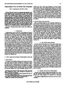
Creation of Sum and Difference Channels

The channels treated in these simulations are not the “ordinary” ones, F L, F R, C, RL and RR as one might have expected. Experience, experiment and tradition altogether have implied that a better idea is to encode the sums and differences of the channels. One explanation to this fact is related to the bit- and coding errors, which in real life are unavoidable. Bit/coding errors or sudden changes in bit rate for a single channel become more obvious to the listener in the case of coding the channels individually. In the sum/difference case possible annoyances will at least be smeared out on two channels which are relatively spread out in space, instead of being placed in one particular loudspeaker. • An example of a person with “experience” is my supervisor, Ingemar Johansson. • Listening tests of rather informal characteristics, of these experiments pointed out that coding the channels in their original configurations re22

sulted in a sound experience with a poorer room definition. A source of a sound could for example tend to give an impression of moving around spatially. This is the “experiment”. • The term “tradition” is motivated by for example low bit rate stereo coders, where the sums are encoded. Furthermore, the classical pilot stereo for FM (Frequency Modulation) radio is a sum/difference coding as well. This information is retrieved by spoken/written conversation with Ingemar Johansson. However, one possible drawback of encoding the sound channels as sums and differences is that the chance for leakage between the channels increases the lower the bit rates are. Propositions of future improvements concerning the sum/difference coding can be found in 8. The sums and differences of the channels used are defined as front sum µ ¶ FL + FR FS = (11) 2 front difference

µ FD =

rear sum

µ RS =

FL − FR 2 RL + RR 2

¶ (12) ¶

and finally the rear difference channel µ ¶ RL − RR RD = 2

(13)

(14)

while the C channel is left untouched. Divisions by 2 are made in order to keep the sample values within the range [−1, 1] in the created sound channels. Sample values exceeding the allowed range would lead to truncation which is an unnecessary source of distortion. Moreover, a division by 2 would anyhow be needed either in the creation of F S, F D, RS and RD or in the reconstruction of the original channel configurations in order not to scale up the amplitudes of the sound by a factor of 2. After receiving the encoded and transmitted data, using the four formulas FL FR

= =

FS + FD FS − FD

RL = RR =

RS + RD RS − RD

(15)

the channels will easily be added and subtracted back into the original channel configurations of the sound.

23

4.2.5

Different Dependency Chains

In the simulations both F S and C was tried out as leading channels with the second channels F D and F S, the third channels C and F D, fourth and fifth channels were in both chains RS and RD respectively. The energy reduction was in general comparable between these two ideas. The idea that will be used and discussed from now on will be the second one. As an attempt of explaining better, the first idea written coarsely as a formula would look like RD RS C FD

∼ ∼ ∼ ∼

RS, C, F D, F S C, F D, F S F D, F S FS

(16)

while the second idea would be looking like RD RS FD FS

∼ ∼ ∼ ∼

RS, C, F D, F S C, F D, F S F S, C C

(17)

using the same way of describing. In the above two formulas, the sign ∼, is representing dependency. A motivation for choosing the second idea is that it is quite common that in movies the main dialog is situated in the C channel. Therefore one would wish to minimize the probabilities of coding errors in that particular channel by making it independent of other channels. 4.2.6

Time Windowing

All decorrelations were performed band wise. For each frequency band one sound channel was predicted from the leading one, a third channel was predicted from the two preceding ones, and so forth. All processing – predictions and energy calculations, was made within certain partially overlapping time windows. These time windows were centred 20 ms from each other, divided by a scaling factor depending on the ISF mode of the coder. Scaling factors belonging to which ISF (here, ISF means Internal Sample Frequency) mode can be found in table 1. In order to make the transitions between each time segment as smooth as possible, their actual lengths were set to be 30 ms, giving symmetric 5 ms overlaps in the beginning and at the end of each time window. In order to preserve the energy (in the overlaps) and make the transitions smooth, each

24

time segment was multiplied by the window function  ¡ ¢ £ π π¤  sin2 t + π4 £, t ∈ − ¤ 4, 4 π 3π w (t) = 1, t ∈ , ¡ ¢ 4 4 £ 3π 5π ¤  cos2 t − 3π 4 ,t ∈ 4 , 4

(18)

where π2 is related to 10 ms of time. These time windows were used both for the frequency domain and time domain predictions. A visualization of w (t) can be found in figure 14. Band Dependent Window Sizes in the Time Domain In the time domain case band dependent lengths of the time windows were also tried. For the first band a time window was 80 ms, 40 ms for the second band and in the third frequency band the length of the time windows were put to 20 ms. The simulated results were roughly the same as in the case of time windows of equal sizes of 20 ms. A motivation for this check is that with too short time windows the frequency resolution is not fine enough to solute the low frequency components in a descent manner.

25

w(t)

1

0.8

0.6

0.4

0.2

0

0

0.5

1

1.5

2

2.5

Figure 14: The time window w(t), where

4.2.7

3 π 2

3.5

4

4.5

≈ 1.57 corresponds to 10 ms.

Time Domain Decorrelation

In the particular case where C was the leading channel, C would be encoded to ˜ F S is decorrelated to and received as C. l−1 z}|{ X F Sn = F Sn − ak Cñ−k

(19)

k=0

where l is the length of the predictor. The reason why to decorrelate F S using C˜ instead of C is related to error propagations. On the receiver side, the only information available about the centre channel is the compressed version of it, ˜ This means that C˜ is the encoded signal that after transmission also denoted C. is decoded. On the other hand, at the encoding/sending side of the transmission both C and C˜ are available. Decorrelating using the compressed versions of the leading channels is thus wiser in the purpose of minimizing the propagation of errors. Naturally C 6= C˜ in general, and therefore decorrelating F S using C instead of C˜ would increase the risks that z}|{ FS (20) 26

later on would be reconstructed slightly worse than is needed for a given bit rate. Further down in the dependency chain the errors might grow bigger since these channels depend upon so many others. Please, note that one can not expect an encoded reference channel to be as efficient as a predictor as a non-coded one. Nevertheless, less sound distortion is preferred compared to risking a more distorted sound, even if it would possibly mean a more efficient decorrelation the channels in between. Please note, as the observant reader already might have done, that in this illustration/example the prediction is only performed backwards in time. In the case of predicting for the same distance in both directions of time, k would run l−1 from 1−l 2 to 2 , for l odd and positive. In cases when l is an even number, the “two-directed” prediction would not possibly be able to be exactly symmetric. However, that consideration is of minor/negligible significance in real life. The predictor coefficients, ak , of the dependent channel F S will be deter2 mined by minimizing |formula 19| . Thus, the relation of equation 19 is representing an ordinary MMSE predictor. In a similar manner F D is decorrelated according to l−1 l−1 z }| { X X g F Dn = F Dn − bk Cñ−k − bl+k F S n−k k=0

(21)

k=0

again by the principles of the linear MMSE-predictor, where actually the prediction error is what is encoded and transmitted. Further on, equation 21 is z}|{ g valid, under the convention that the coding of F S will give F S which later on will be transmitted to the receiver. The received signal regarding F D is cong sequently denoted F D. This one is used in a similar manner for decorrelating the RS channel and so forth. Since the idea keeps the same, but the formulas are getting lengthier, the formulas for the two last channels are left out and the still confused reader might refer to figure 15. In the diagram of figure 15, the block “Coder” is representing both encoding and decoding. In this text the encoded signal (the one transmitted) and the thereafter decoded signal (the one used as reference, which is the one available after decoding the received signal) are treated as one and the same for conceptual convenience. The reason to encode and decode the signal before using it as a reference for the decorrelating predictor is explained in the beginning of this sub-subsection of the thesis.

27

C

FS

FD

RS

RD

Coder

+ a C

−

Coder

+ b FS

− + b C

−

Coder

+ c FD

− + c FS

− + c C

−

Coder

+ d RS

− + d FD

− + d FS

− + d C

−

Coder

Figure 15: Diagram describing decorrelation of the channels as performed in the time domain. The C channel is leading; the remaining channels are dependent in a chainlike structure. The “Coder” blocks are representing both encoding and thereafter decoding of the encoded signal. The labels on the decorrelating filters tell the following. The first row; a predicts F S, b predicts F D, c predicts RS and d predicts RD. On the second row of the labels of the filters one can read which sound channel that is used for decorrelation.

28

4.2.8

Time Domain Reconstruction

The reconstruction of these channels will now be explained. In the simplest case, the centre channel, the reconstructed Cˆ is exactly equal to the received C˜ since this was chosen to be the leading channel. F S is reconstructed by the mechanism obeying the d g F Sn = F Sn +

l−1 X

ak Cñ−k

(22)

k=0

formula. This in turn gives for the front difference channel this reconstructing scheme l−1 l−1 X X d g g F Dn = F Dn + bk Cñ−k + bl+k F S n−k (23) k=0

k=0

and in order to further clarify, both the rear channels’ reconstruction schemes are stated cn RS

=

fn+ RS

l−1 X

ck Cñ−k +

k=0

dn RD

=

gn + RD

l−1 X

+

g cl+k F S n−k +

k=0

dk Cñ−k +

k=0 l−1 X

l−1 X

l−1 X k=0

l−1 X

g c2l+k F Dn−k

(24)

k=0

g dl+k F S n−k +

l−1 X

g d2l+k F Dn−k +

k=0

f n−k d3l+k RS

k=0

an by now, the pattern ought to become obvious. For a visualization of the reconstruction of the channels, the reader is advised to examine the figure 16 ˜ F S means F g diagram. Please note that in figure 16 C actually means C, S and so forth. This aesthetical and pedagogical inconvenience is due to technical limitations in the graphical software used (Dia).

29

C a C

FS

+

b C

c C

+

b FS

FD

d C

+

c FS

+

+

d FS

+

c FD

RS

+

d FD

+

+

+

+

+

d RS

+

RD

+

+

+

+

+

+

+

Figure 16: Reconstruction of each channel of the signal by adding the decorrelated channel to filtered versions of the channels it is depending upon. Please ˜ F S means F g note that C actually means C, S and so forth. This aesthetical and pedagogical inconvenience is due to technical limitations in the graphical software used (Dia).

30

4.2.9

Two Smaller Dependency Chains

Since the in the above described chains of predictions gave rise to quite many predictor coefficients to transmit, yet another idea was tried out. The number 4 P of predictors in the prior model are i = 10, times the length of the predictors i=1

times the number of frequency bands. The other, more economical method was based on the assumption that the three front channels had more in common together than what they had in common to the two back channels. Naturally, the inverse relation was assumed in the model as well. By letting F S and RS lead each subgroup and F D, C respectively RD be the followers, see figure 17, one now has two shorter prediction chains instead of one longer. This idea would reduce the predictor coefficients to transmit to 2·1+ 2 = 4 times the length of the predictors times the number of frequency bands. Generally though, it seemed that the dependencies the channels in between were not restricted to any certain directions. Therefore this model was not as efficient as was hoped for. Everything depends on how the material is mixed and/or recorded. There seem to be no general truths about multi-channel audio.

31

FS

Coder

a FS

+

FD

b FS

-

Coder

b FD

+

C RS

-

+

-

Coder

Coder

d RS

RD

+

-

Coder

Figure 17: The alternative decorrelation model, based on assumption of looser relations the front and back channels in between.

32

4.2.10

Additional Ideas Regarding the Decorrelation Efforts Made in the Time Domain

All along the feasibility studies it became obvious that the existence of interchannel dependencies is quite material dependent. When all is said and done, finally, the properties of a piece of sound depend on the mixing of the sound. Regarding movie audio, there are at least certain vague borders to stay within in order not to upset the audience. In the case of music videos on the other hand, the artistic freedom composing the sound mix is even bigger than for the movie audio mixing. The imagined listener can be placed in the centre of, in front of, above and even in other indeterminable positions in relation to the playing band. Anyhow, several ideas has been tested in order to see if there existed any decorrelation method that would be efficient enough for a general 5.1 recording (for explanation about 5.1 audio, see 1.1) to overweight/compensate for the extra cost in bit rate caused by the transmission of the predictor coefficients. Longer Predictors One of the ideas tested was to try different predictor filter lengths, and as one can expect, longer filters did result in less energy of the decorrelated channels. But the increase of reduction of energy was in most of the cases small, so small that one would need to let the resulting energy plots overlay each other in order to make the difference noticeable. These longer predictor filters were tested to act both backwards in time as well as symmetrically backand forwards in time, as briefly described earlier in this thesis. For predictors of same lengths, in most of the cases the one predicting in both directions exhibited a slightly better performance than the one predicting backwards in time only. Anyway, since the differences were merely measurable compared to filters of one coefficient, usage of longer filters could not be motivated. Obviously, the most efficient way to predict one channel from the other(s) was with a one tap filter acting on the channel(s) of greater importance at the same moment in time. From this on the length of the filters were limited to one coefficient merely. This means that a channel of sound, at a certain frame in time, is modelled to be dependent only of the state(s) of the other channel(s) at the same time frame as the channel in question. One Coefficient Predictors In order to improve the performance of the one coefficient predictor described above, one effort was implementing the possibility to translate the predictor back and forth in time. Here, the time translation k was represented by seven bits. This means that each predictive filter looked like h [n] = a · δ [n − k]

(25)

where a ∈ R for an unquantized a, k ∈ Z ∩ [−64, 63], n ∈ Z, and δ [n] is the discrete counterpart of Dirac’s delta function, the so called Kronecker delta which attains the value 1 for n = 0 and 0 for n ∈ Z\ {0}.

33

This method was (at least in Matlab) quite slow, since it had to determine k before calculating the predictor coefficient. Comparison of the absolute values of a vector of correlation coefficients, like equation 72, was a necessary step in the procedure of determining the optimal time translation for each leading channel. One such vector was computed between the channel to decorrelate and each channel it was modelled to be dependent upon. Each one of the X’es of equation 72 represents in this case one of all the 128 possible time translations of the leading channel. The time shift that resulted in the maximal absolute value of this vector was set as k. Unfortunately any greater gain in energy reduction was hard to notice, the results were about the same as for the k = 0 case in the simulations performed. 4.2.11

Frequency Domain Decorrelation

Decorrelation attempts were also performed in the frequency domain. The frequencies were split up into ten frequency bands. In the case of 6 kHz band limitation, the 20 first critical bands of [Painter, Table 1] were used pair-wise. A band limitation of 8 kHz was also tried out. In the latter case the critical bands from 1 to 16 were used pair wise, and the critical bands 17 − 19 and 20 − 22 constituted the two last frequency bands in the simulation model. FFT For each time window, an FFT was calculated. The time windows of equation 18 used when working in the frequency domain are the same as those described in connection to the time domain decorrelations. FFT means Fast Fourier Transform, which is simply a fast numerical algorithm calculating the DFT, the Discrete Fourier Transform. The DFT, Xk of a sequence xn is defined as Xk =

N −1 X

e

−2πikn N

xn

(26)

n=0

where N is the length of the sequence. Inverse formula of the DFT is defined as xn =

N −1 1 X 2πikn e N Xk N

(27)

k=0

whose fast counterpart is called the IFFT (Inverse Fast Fourier Transform). There are other variants of scaling the FFT and IFFT, but Matlab uses the two above described formulas [FFT]. In the formulas of equation 26 and equation√27 above, of course i denotes the unit for imaginary numbers, © defined as i = ª−1. For (real valued xn and) N even Xk is unique for k ∈ 0, 1, ..., N2 − 1, N2 only, while Xk = XN −k for k > N2 . This feature is of course taken advantage of in the predictor calculations. The coefficient representing the lowest frequency, that is 0 Hz or historically DC, is represented by k = 0 and the highest represented frequency, f2s , by k = N2 . 34

Coefficients placed in between N2 + 1 and N − 1 represent the “negative frequencies”, a mathematical rather than physical concept – nevertheless important enough not to be disregarded. Moreover, the modulus of each FFT coefficient corresponds to the amplitude of the frequency (or rather in case of FFT/DFT, span of frequencies) it represents. At the same time the angle in the complex plane of each FFT coefficient represents the phase shift of the corresponding harmonic in the time domain. Decorrelation within a Frequency Band As well as with the decorrelation by MMSE prediction in the time domain, the centre channel was chosen to be the leading channel. The F S channel was for a specific band X decorrelated as z

}|

{

F F T band X F Sn

=

F F T band X F Sn

−

l−1 X

ak

^ FFT band X Cn−k

(28)

k=0

where k, n ∈ Z should be regarded as time frame indices. Even if the possibility exists predicting over several time frames, in the simulations performed for this thesis l always equalled 1. A similar idea was applied for the F D channel z

}|

{

F F T band X F Dn

=

F F T band X F Dn

−

l−1 X

bk

^ FFT band X Cn−k

k=0

−

l−1 X

^ FFT band X bk+l F Sn−k

(29)

k=0

g and the pattern continues on for the rest of the channels. F S, using the same notation as in the time domain discussions, is created by putting all the z

}|

{

F F T band X

FS

(30)

for each band together, like   z }| { z }| { z }| { z }| { z }| {  F F T band 1 F F T band 10 F F T band 10 F F T band 9 F F T band 1 FS , ..., FS , FS FS , ..., FS , except 0 Hz   f lipped except f2s Hz   f lipped

(31)

f lipped

inverse transforming the sequence of complex numbers of equation 31 and thereafter coding and transmitting it. Each one of the frequency bands that are complex conjugated needs to be flipped around as well, so that its representation is reversed. This means that the FFT coefficient representing the highest frequency in the band will come first, and the FFT coefficient of the lowest g frequency in the band will come last. Now that F S is computed, ^ FFT band X FS

(32)

is easily extracted for further decorrelations by Fourier transforming and band g separating that signal F S. For more details, see figure 18. 35

C

FS

FD

RS

RD

Coder FFT

Transmission

FFT

FFT

FFT

FFT

+ a C

−

IFFT Coder Transmission

FFT

+ b FS

− + b C

− Cutoff

Transmission

FFT

The diagram continues in the following picture

Cutoff

Coder


IFFT

Cutoff


Cutoff


Figure 18: Decorrelation of the channels as it was done in the frequency domain. Note that the “Coder” blocks represent both encoding and decoding of the signal. Also note that the “Transmission” arrows are supposed to contain the encoded but yet not decoded signal. The latter remark is quite logical, though the sketch might be ambiguous to an outsider to the problem formulation. The figure is split into two pieces, where this is the first one and figure 19 is the second one. 36

Cutoff

c FD

−

+

c FS

−

+

c C

−

IFFT

Coder

Transmission

FFT

+

d RS

−

+

d FD

−

+

d FS

−

+

d C

−

IFFT

Coder

Transmission

37

The diagram continues from the preceding picture

+

Cutoff The diagram continues from the preceding picture

Figure 19: The figure is split into two pieces, where this is the second one and figure 18 is the first one. In the caption text of the first one the description can be found.

4.2.12

Examples of FFT Domain Decorrelation

An example of a sound clip that is relatively easy to decorrelate is “Only the Lonely” from Roy Orbisons DVD album “A Black and White Night”. A plot of the energy reductions made in the 6 kHz band limited case, using the predictor model of Yˆ as described in formula 52 for each frequency band, predicting at the same time frame only, can be found as figure 21. The a of formula 52 is real valued, while of course the Y and X:s are complex valued. The x axis of the plot represents each time frame, while the y axis represents the relative energy of each channel compared to the non-decorrelated case. Energies are expressed in dB. Each time frame has the familiar length 20 ms divided by the proper scale factor. In the case of 6 kHz band limited signals, the associated scaling factor equals 0.9375. Another example, this time on a sound clip with a more ordinary behaviour is found as figure 20. Comparing the latter illustration, which is taken from a sound clip of Chapter 20 in the DVD movie “Pearl Harbor”, with the one of figure 21 might give a rough idea of the difference between a sound clip that is worth decorrelating by prediction before coding and one that certainly is not. Further graphical examples from the simulations of energy reductions performed in the frequency domain are the pictures of figure 22 as well as of figure 23. The model behind the first one of these, equation 60, is the one with two different predictors, where the real and imaginary parts of the FFTs of the signals are assumed to be independent of each other. In order to clarify, the real/imaginary part of the FFT of a dependent channel is assumed to depend on the real/imaginary parts of the FFTs of the leading channels only. As can be seen in the picture of figure 22, simulations have shown gains in energy reduction for all the dependent channels compared to the model of equation 52 where a ∈ R merely. Naturally the axes of the graph represent the same entities as in the case of figure 21. Results from the simulations regarding the most general model implemented for decorrelation in the frequency domain, equation 61, can be found in figure 23. Of course this figure is representing simulations of the same sound clip as in the two previously presented plots of figure 21 and figure 22, otherwise no relevant comparisons would be possible to make. This model, the one of equation 61, is a generalization of the former model. Here both the real and imaginary parts of the dependent channels are assumed to depend upon the real as well as the imaginary parts of the channels higher up in the dependency chain. In several cases this model ends up with either bad references or with correlation matrices so badly conditioned that in the last step, the decorrelation of the RD channel, the energy reduction is bad compared to figure 21 and figure 22. Sometimes for the RD channel, the energy reduction is even close to or equals zero. A somewhat deeper discussion about this phenomenon can be found in 4.2.13. In short; the presumed cause of the phenomenon is that an encoded version of a leading channel decorrelates the dependent channel less efficient than a non-encoded version. This model is outperforming the other models concerning the other channels’ decorrelations as can be seen in the figure.

38

The Front Difference Channel 0 −10 −20 0

50

100

150

200 250 300 The Front Sum Channel

350

400

450

0

50

100

150

200 250 300 The Rear Sum Channel

350

400

450

0

50

100

150

200 250 300 350 The Rear Difference Channel

400

450

0

50

100

150

200

400

450

0 −10 −20

0 −10 −20

0 −10 −20 250

300

350

Figure 20: An example of a clip from Chapter 20 of the motion picture Pearl Harbour that is decorrelated. The decorrelations were performed in the frequency domain (0 − 6 kHz), with one real valued predictor for each leading channel and band. The amount of linear dependencies the channels in between of this illustration is quite representative for most of the signals used in the simulations.

39


50

100

150


350

400

450

0

50

100

150


350

400

450

0

50

100

150


400

450

0

50

100

150

200

400

450

0 −10 −20

0 −10 −20

0 −10 −20 250

300

350

Figure 21: Decorrelating example (Roy Orbison – Only the Lonely) performed in the frequency domain (0 − 6 kHz), one real valued predictor for each leading channel and band.

40


50

100

150


350

400

450

0

50

100

150


350

400

450

0

50

100

150


400

450

0

50

100

150

200

400

450

0 −10 −20

0 −10 −20

0 −10 −20 250

300

350

Figure 22: An example of a short clip out of Roy Orbison – “Only the Lonely” decorrelated in a more sophisticated way. The decorrelations were performed in the frequency domain (0 − 6 kHz). Here, one predictor is used separately for the real and imaginary parts of each leading channel and band respectively.

41


50

100

150


350

400

450

0

50

100

150


350

400

450

0

50

100

150


400

450

0

50

100

150

200

400

450

0 −10 −20

0 −10 −20

0 −10 −20 250

300

350

Figure 23: Decorrelating example of a short clip out of Roy Orbison - “Only the Lonely” performed in the frequency domain (0 − 6 kHz). In this case, two predictors are used for each leading channel and band. One predictor is used for the real, and one is used for the imaginary part. Naturally, the real and imaginary parts of a depending channel have different predictors. This gives four predictors for each pair of channels.

42

4.2.13

Bit Rate Allocation and Reference Channel Puzzles

In the decorrelation process described above, there is one inherited problem. This problem is present in the time domain decorrelation as well. The optimal bit rate in which to encode each sound channel is determined, or rather estimated, from the energies of the decorrelated channels using non-encoded channels as references. This is done because in the beginning there is nothing else to estimate from. A reference channel that is distorted by coding might reduce (or at least in some way influence) the ability to decorrelate the other channels. The more distorted a sound is by coding, the less suitable as a predictor for a non-distorted sound it is. This in turn leads to channels that will not be energy reduced in the amount estimated. Consequently, such a channel will then be compressed in a bit rate related to a lower energy than the actual energy of the channel. In the next step, the decorrelated, encoded and thereafter decoded channel will be an even worse predictor for the remaining channels than the predictors of that particular channel were. The above described phenomenon becomes more and more pronounced the further down in the dependency chain a channel is situated. Another amplifier of the phenomenon is of course to lower the bit rate of the encoder. As a matter of fact this tendency is as most obvious in the cases of relatively efficient decorrelation. One can get quite a good visualization of this phenomenon by comparing figure 21 and figure 23 who are examples of the energy reduction results applying the frequency domain decorrelation ideas of formulas 52 (with a ∈ R) and 61 respectively. Note that even though the prediction model of equation 61 is more efficient on average, for the RD channel the performance is worse than in model using equation 52. If the above described phenomenon was the only explanation to the results attained, an attentive reader would have asked himself/herself why the RS channel is decorrelated as good as it is. Therefore some complementary explanations will be revealed below. If the following ideas about the phenomenon are correct or not is hard to state. Nevertheless they contain relevant ideas and might at least be treated as seeds for future answers. Even though it can be considered quite unrealistic that the channels are fully decorrelated in the RD channel when decorrelations are bad, that is indeed a possibility. Rather, a qualified guess would be that for many time frames the correlation matrices, R, are so badly conditioned that no decorrelation at all is performed. A possible remedy to that problem could be reducing, or at least modifying the dependency chain. That would give us smaller, or at least other, correlation matrices – hopefully better conditioned. Anyway, the phenomenon is mentioned and some possible explanations and remedies were presented, but no efforts have been done solving the problem for this thesis.

43

4.2.14

FFT Domain Reconstruction

In this piece of text, the method used for the reconstruction of the received signals when decorrelating in the FFT domain will be presented. Since the centre channel is the leading one, its reconstruction is already done when it is been received (decoding excluded). In the case of F S, for each time window, the received signal is Fourier transformed and band separated. With the same notation as in the case of time domain decorrelation \ FFT band X F Sn

=

^ FFT band X F Sn

+

l−1 X

ak

^ FFT band X Cn−k

(33)

k=0

and, when all the bands are done, an inverse transformation will be performed to d create F S. As well as in the time domain case, the time windows are somewhat overlapping in order to avoid noticeable discontinuities in the sound waveform. Regarding the other channels, the reconstruction procedure is similar. For a more detailed description, please refer to the diagram of figure 16 in which the main idea is the same except that before applying the recorrelation filtering the received signal needs to be Fourier transformed and divided up into the ten frequency bands presented earlier. 4.2.15

Experiments Using the HF Part of the Front Channels in the Rear Channels as Well

Efforts aiming to reduce the over all bit rate further were performed by replacing the FFT coefficients of the higher frequencies (of the low pass filtered signal) of the two rear channels with the ones from front channels. When using the centre channel, the HF parts of both the rear channels were replaced with the HF parts of the centre channel. In the case using the F S and F D channels, naturally the HF parts of F S replaced the HF parts of RS. Likewise was done for the difference channels. A visualization of figure 24 may be consulted by the still confused reader. In listening tests, none of the two methods resulted in any enjoyable experience or similarity to the original sound at all. If having to choose one of the two substitutions tried, the latter one would be the preferred one. In the case of replacing the higher frequencies’ FFT coefficients of RS with the ones of F S and the coefficients of RD with the ones of F D the output was less different from the original sound than in the case of using the centre channel. A possible explanation for this result might be that in the sounds tested the correlations between the sum channels and difference channels respectively were somewhat higher than the correlations between the centre channel and the rear channels. Concluding that these ideas could be considered as bad, they were discarded after the experiment made.

44

FFT coefficients of FS

DC

...............

...............

...............

...............

Useful Bandwidth

Useful Bandwidth

Useful Bandwidth

Useful Bandwidth

FFT coefficients of FS

DC

FFT coefficients of FD

DC

FFT coefficients of RS

DC

FFT coefficients of RD

DC

...............

...............

...............

...............

Useful Bandwidth

Useful Bandwidth

Useful Bandwidth

Useful Bandwidth

45

FFT coefficients of FD

DC

FFT coefficients of RS

DC

FFT coefficients of RD

DC

Figure 24: An example of the not-so-well-working ideas of replacing the FFT coefficients of higher frequencies of the rear channels with coefficients of the front channels. In this example F S and F D are used. The case is quite similar when using the C channel instead.

4.2.16

FFT Domain Results

The results of frequency domain decorrelation (using the real valued predictors a of equation 54) showed a slightly better performance in relation to the results of the time domain simulations. In a majority of the cases, the frequency domain method, on average, performed somewhat better compared to the time domain method. On the other hand, the greatest moments of energy reduction were not as great as the greatest moments in the time domain case. In order to clarify, for specific frames of time the energy reduction in the time domain decorrelations could be tremendously higher than for the frequency domain decorrelations. On the other hand, still, the decorrelations made in the FFT domain were performing better on a time frame average. This might be interpreted as a combination of an in-time-smearing and a slight improvement of performance relating the FFT domain decorrelation to the time domain decorrelation. One possible explanation of the tendency of better performance of the frequency domain method can be as simple as that the spectrum is divided into a lot of more bands in this model than in the time domain prediction model. This in turn leads naturally to a greater number of prediction coefficients. Not even a rough guess regarding the reason for the in-time-smearing of the performance of the FFT domain decorrelation, compared to the time domain decorrelation case, will be done in this thesis. The making of such an explanation is a serious task and will therefore not be done. Finally, even if the FFT domain was a better environment to decorrelate within, it was not good enough. And maybe it was better, since it was also faster than the time domain methods – at least as they were implemented in Matlab. Reconsider the figure 20 which was a representative example the energy reduction of many 5.1 sound clips tested. This is obviously not enough for using the decorrelation ideas in the coder. Especially not when taking the risks of distortion propagation between the channels into account, spreading caused by for example a damaged reference channel that is located quite high up in the dependency chain. Another disadvantage using decorrelation is that the method is quite complex. Furthermore the encoding, decoding and decorrelation procedures will definitely give rise to delays of the coder. Delays that won’t be acceptable for all kinds of applications.

4.3 4.3.1

Modifications of AMR-WB+ needed to be made Introduction

Since it was concluded that decorrelation of the channels using prediction was contra productive in general, no such things were implemented in the C code. Nevertheless, the two simple and similar bit allocation methods, the ideas of equation 35 and equation 37, was implemented. The same bit rate allocation models were naturally used in the Matlab simulations as well. The LF E channel was not included in these bit allocation methods because of the “oddness” of the channel. The compression of the bass channel was taken care of separately, and will be described right away in the following sub-subsection of the thesis. 46

The migration of the work from the cosy Matlab environment to the more brute C world was mainly motivated by the three following reasons. • Firstly, since Matlab which called upon DOS boxes with the coder (mono mode of AMR-WB+) needed to keep all the data in its own memory the lengths of the sound clips for processing and listening were rather limited. The already existing C program did of course not keep more of the sound clip in the memory of the computer than needed for processing. All data not needed for the moment is as one can expect continously written out on disk. • Secondly, in order to get the total sound experience, the BWE (BandWidth Extension) of the coder needed to be used. BWE is a method of coding the higher frequencies of the sound that can be found described more extensively in 3.6. There was a need to code the HF (high frequency) parts of the signal on the original channels, and not on any constructed differences and sums of them. A simple call from a Matlab script to the mono coder could not possibly satisfy the need for coding the LF (low frequency) parts from one source and the HF parts from another one. • Thirdly, after finalizing the simulations, it is always nice to have a real working program available for presentations. That means something that at a greater extent seems like a real product. Thus, to start digging into the C code was a must from “here” on. A description of the more important changes that have been made will follow. In this thesis work, only the mono coding modes should be used. Therefore, the first modification that was made in the program in order to reduce the amount of expendable code was removing all the stereo coding modes of the coder. This in turn increased the ability to get an overview of all the remaining parts of the coder. In addition to that, the program was modified to be able to handle audio files containing six channels. For the multi-channel AMR-WB+ mode, the input for the encoder is six channel WAV files with 16 bits per sample. These WAV files are sampled at a sample frequency, fs , of 48 kHz. The compressed output is stored in a special parametric format. The decoder extracts the compressed parameter file back to the well known WAV format for listening. 4.3.2

The Bass Channel, Also Known as the Low Frequency Element (LFE)

Thanks to the relatively heavy band limitation (as well as the lack of transients) of the LF E, the bit rate demands for the bass can definitely be considered as small compared to the “ordinary” sound channels. In the current solution, the 120 · scaling bps. For the specific bit rate of the bass channel is computed as 0.08 120 · 1.5 = 2250 bps, that case of ISF = 12, the bit rate of the LF E ends up at 0.08 is ∼ 2.3 kbps. The number of LF E bits is quite generously allotted and might 47

be an issue of reduction. On the other hand 2.2 kbps is nothing compared to the to the bit rates of the music sound channels. Thus further bit rate reduction of the LF E is not a number one priority. The coding of the LF E channel is a simplified case of the LF coding of the other channels. Naturally no BWE is performed. For the bass speaker sound coding, the only coder mode that is used is the TCX80 mode. That is quite logical since there are only slowly varying, low-frequency, music-like sounds, and hardly any presence of transient sounds at all in that channel. Moreover, since the values of the FFT-coefficients representing the higher frequencies, would (if they were used) be zero, or at least so close to zero that they could be neglected, only the first three of the 144 eight-dimensional vectors of FFT coefficients is used by the TCX coder. This means, taking two examples, that for ISF = 12 3 3 the LF E is band limited to 9600 · 144 = 200 Hz, and for ISF = 7 to 6000 · 144 = 125 Hz. (Here ISF means the Internal Sample Frequencies to be found in table 1.) High pass filtering at 20 Hz would at the best not affect the sound at all, but it is likely to ruin, or at least mutilate, the LF E signal. Hence, no high pass filtering is done on the LF E sound channel. Furthermore, neither any pre-emphasis, nor the LPC analysis is needed here. Obviously, the narrowness of the spectrum of the sound contained in the LF E channel leaves hardly any spectrum to flatten out. Thus, no LP coefficients need to be transmitted for the bass channel and thus some extra bits are saved per “super frame”. As a consequence, no ISF (in this case the acronym stays for Immitance Spectral Frequency) domain transformations are needed either, reducing the complexity somewhat. 4.3.3

The Addition of Six Extra Low Bit Rate (TCX) Modes

The bit rates listed in table 2 are not the original bit rates only. The six lowest bit rate modes in table 2 (the ones written in an italic font) were added to the ones of the original mono coder. Details about the original coder are of course found in [26.290]. Usage of the lowest bit rate modes are mainly intended for pieces of sound that are almost silent or have vanishing low energies (in a relative measure). There is one main difference between the new modes and the old ones, the bit rates disregarded. While the old bit rates allow using all the four coding modes described in 3.1, the new low bit rate modes utilize only the three TCX modes available. The above declared addition of extra bit rates is justified in what follows. Just letting a sound channel abruptly go to zero, for a certain time frame, is more destructive to the impression of the sound than to gradually lower the bit rate to ridiculously low levels. This means levels that in any case would not steal so much bit rate from the more relevant channels. This method gives more of continuity to the sound, which means that, as an example, snaps in the sound when switching the sound on and off is avoided. Besides that, listening tests has showed, that even in cases where a sound channel produces mostly gibberish it has a positive contribution to the room experience, in combination 48

with the rest of the sound channels of course. 4.3.4

BandWidth Extension (BWE)

As indicated earlier, in the previous subsection, thanks to the rather destructive behaviour of the BWE, modifications of the encoder/decoder had to be done. Suspicions resulted in a minor investigation that took place. Suspected was that when using the BWE technique, the coding of sums and differences instead of the original channels would give rise to problems. Comparisons comprised listening tests as well as contemplation of the sample values. As expected, the investigation pointed out that the channels need to be encoded as they are configured from the first start in the HF case, rather than coding the created difference and sum channels processed by the LF coder. All this toil was necessary for the purpose of reducing channel leakage and avoiding unnecessary distortion. Thus, the original C program was modified such that the possibility to encode the HF and LF parts of the sound out of different data sources (left and right channels for the former case, as well as sums and differences for the latter) was supplemented. When a sum channel is encoded in LF, both the left and right channels’ HF parts are being encoded. On the other hand when a difference channel is LF encoded, no BWE is encoded at all. For the centre channel, the encoding is still performed as would be considered “normal” by an old version of the AMR-WB+ mono coder. 4.3.5

The Noise-fill Feature of the Decoder

Another modification that had to be done for the multi-channel decoder is regarding the “noise-fill” feature. In cases when both the sum as well the difference channel produce noise in the holes of the spectrum, using the noise-fill technique, there is a peril that these holes coincide. For noise-fill, where the frequency bands containing the additional noise of the sum and difference√channels coincide, the resulting noise energy per left/right channel will grow 2 times. Addition and subtraction of the sum/difference channels in order to recreate the left/right channels results in addition of noise. Since noise is by definition independent of everything, cancelling is not an issue. A clarification and motivation of the statement about the increase of a fac√ tor of 2 of the noise energy follows. Assume that the variance V (X) of the zero mean X equals 1. The fact that X is zero mean implies that ¡ noise ¢ V (X) = E X 2 . The variance of the addition X1 + X2 , who both are com-

49

pletely independent of each other by the properties of noise, equals V (X1 + X2 )

= {zero mean} ³ ´ 2 = E (X1 + X2 ) ³ ´ 2 2 = E (X1 ) + (X2 ) + 2X1 X2 = = =

(34)

{independency} ³ ´ ³ ´ 2 2 E (X1 ) + E (X2 ) + 2E (X1 ) E (X2 )

=

{zero mean} ³ ´ ³ ´ 2 2 E (X1 ) + E (X2 )

= =

1+1 2

which in turn gives the energy. √ The energy is simply the square root of the variance, therefore D (X) = 2. Therefore a decision was taken to apply the noise-fill for the sum channel decoding only. That is to say, no noise is filled in for the difference channels. Concerning the C channel, it was naturally left untouched of these changes. Apparently, there now will be certain frequency bands left with no noise-fill at all. That is the case when there are no spectral holes for the sum channel, but holes are present in the difference channel. See case 2 in the first numbered list below. On the other hand, that is considered safer than risking energy levels of noise so high that the noise might drown the useful parts of the sound. An outline describing the current solution can be found in figure 25. Three interesting cases are actually illustrated: 1. One of the empty frequency bands of the sum and difference channels coincide. Here, the missing energy is filled out with noise in the sum channel. Nothing is done to the difference channel. In the left/right channels the energy of this particular band becomes “normal”. 2. For another band of frequencies, there is only zeros transmitted in the difference channel while for the sum channel data is transmitted as usual. Here, generally, the resulting left/right channel sound energies will be somewhat lower than they were originally. Of course there are exceptions resulting in no changes, like for example when left channel equals the right channel. In the exemplified case, the difference channel would have been zero anyway. 3. In a frequency band, there are zeros transmitted in the sum channel, but in the difference channel ordinary data is sent. Here, a slight increment of the resulting left/right band energies must be expected. That is explained in the following coarse example. For simplicity, assume that the left and right channels are independent, and that the sum and difference 50

channels are independent as well. These two assumptions are obviously contradictory, but this is the only model that is somewhat related to reality and still allows simple calculations. Furthermore, assume that the energies of the left and right channels as well as the added noise of the sum channel equal, q and say 1, then the difference channel energy becomes q¡ ¢ are ¡ 1 ¢2 1 1 2 1 √1 . This in turn gives left/right channel + 2 = 2 4 + 4 = 2 q q 1 3 energies of 2 + 1 = 2 ≈ 1.2. This example is naturally not an exact description of the reality, more or less just a hint of how it might be in reality. Nevertheless, since by using this simple noise-adding method the resulting left/right signal energies cannot be “perfect” simultaneously for all the three cases listed here, there is no reason going deeper into more advanced and realistic calculations. One could of course argue that a smarter model could have been implemented. That is indeed true. A model that checks if the sounds of the frequencies that are not stored by F S and F D (or RS and RD) coincide or not, and after determining that, makes a proper decision whether or not to add noise is not at all impossibility. However the time was limited for this thesis work, but it might be an issue of relevance for the future. Possibly, an even wiser idea could be to use the “noise-fill” for both the sum and difference channel, but scaling the added noise by √12 . Then, by making the same assumptions as before (that is the assumptions stated in point 3 in the first numbered list of this section), one gets two cases: 1. Where the empty frequency bands coincide, noise would be added for both the sum and the difference r channel. Then the energies of the left/right q ³ ´2 ³ ´2 1 1 √1 √1 + = channels would be around 2 + 2 = 1, which is 2 2 exactly what is whished for. 2. Where there is normal sound in one of the sum/difference channels, and added noise of energy √12 in the other. Then the resulting energy of the left/right channels will equal 1 as well. That is so because the energy of the channel containing the normal sound has the energy √12 as well. A justification of this later statement can be found under point 3 in the prior numbered list. However, the differences between the ideas used and the ideas proposed in this piece of text can be very subtle, and no tests have been performed comparing them.

51

Energy

Left channel

Right channel

Sum channel

Energy

Energy

Difference channel

Frequencies, DC to fs/2.

Energy




Figure 25: A comprehensive sketch of how the “noise-fill” is implemented. Scrutinizing spectators might find several misleads and/or contradictions. Nevertheless, this draft is supposed to serve as a nice simplification – no more, no less. Black colour indicates spectral holes that are filled with noise. Discussions will be found in the sub subsection of “The Noise-fill Feature of the Decoder”.

52

4.4

Bit Rate Allocation

Summing over all the channels to be encoded and transmitted, the bit rate is kept approximately constant in time. Individually though, the bit rates are time variant for each channel. For each time window w (t) of equation 18 a new bit rate distribution amongst the channels is calculated. Two models have been tested, both of them depending on the energies, E, of the channels. In the first model, equation 35, the bit rate, BR, for a specific channel k is ideally Ek BRk = P BRtotal (35) En n

but since the available bit rates of the coder constitute a finite set (there are 14 different ones available, see table 2) of bit rates, the BRk will be quantized at some extent. Let Q (BRk ) denote the quantized versions of BRk . Summation over all the channels, like X Q (BRk ) (36) k

will result in total bit rates that are either far too high, far too low, or in total bit rates that are landing in the specific range that is considered acceptable. Thereafter, in cases of bit rate sums localized outside the accepted range, iteration is possible. By scaling all the BRk s up or down (by factors like 1.1 and 0.9 respectively) and thereafter requantizing them a couple of times, the sum of equation 36 will hopefully be as close as wished for, in relation to the desired value of BRtotal . In cases where a scaling of the BRk s will give rise to changes of the Q (BRk ) values for two or more of the channels the iteration might not converge if the allowed span of fluctuations in bit rates around BRtotal is too narrow. This phenomenon might occur in cases of several channels with the same amount of energy. For example if two of the transmitted signals are silent at the same time. Handling this problem is beyond the scope of this thesis, but a possible solution could be to allow for greater fluctuations in total bit rate if the number of iterations exceeds a specific predefined value. Moreover, an implementation controlling a moving average of the bit rates could lower and raise the desired BRtotal in order to avoid overflowing or flushing the buffers during the transmission. An example of the bit rate distribution for the model of equation 35 is visible in figure 26. The second model, formula 37, is basically the same as the first one except that it generates a denser distribution of bit rates among the channels. In this case the ideal non-quantized bit rate allocation will obey ln (1 + Ek ) BRtotal BRk = P ln (1 + En )

(37)

n

where the addition of 1 to E is needed in cases of energies 0 ≤ E ≤ 1, because taking the logarithm of E, 0 ≤ E ≤ 1, would produce great negative numbers or zeros. The former is a problem since negative bit rates are nonexistent, while 53

the latter might cause severe problems in the denominator. An illustration of the denser bit rate distributions can be found in figure 27. This might be put in relation to the results of the former model, revealed in figure 26. Both of the figures describe the bit rate distributions for the same piece of sound (a short clip of “Only the Lonely” from Roy Orbisons DVD album “A Black and White Night”) and the same desired BRtotal , that is 80 kbps (excluding the LF E bit rate). For further comparisons between the two models, the figures 28 and 29 can be studied. Both of them are visualizing the bit rate distributions for a shorter clip out of Chapter 20 of the DVD motion picture “Pearl Harbor”. Also here, BRtotal is set to 80 kbps. The first of the two figures represents the proportional way of distributing the bit rates while the second of them represents the logarithmic way. The characteristics of each distribution are still familiar, but some differences between a movie and a piece of music can be found. To take an example – the centre channel plays a more dominant role in a movie in general than for music. Please note that the distributions visualized in figures 26 - 29 might seem more evenly spread than they actually are, and that depends on the 10 frames moving average filtering. It would however lead to other difficulties interpreting the figures if the plots were not evened out in time.

54

35

30

bitrate [kbps]

25 FS FD C RS RD

20

15

10

5 50

100

150 frame

200

250

Figure 26: Example of bit rate allocation for a desired total bit rate of 80 kbps using the energy proportional bit rate allocation method. The graph of each channel is evened out by a 10 frames moving average filter. This is a clip out of Roy Orbison’s “Only the Lonely”, on the DVD album “A Black and White Night”.

55

FS FD C RS RD

35

30

bitrate [kbps]

25

20

15

10

5 50

100

150 frame

200

250

Figure 27: Example of bit rate allocation for a desired total bit rate of 80 kbps using the logarithmic energy proportional bit rate allocation method. The graph of each channel is evened out by a 10 frames moving average filter. This is a clip out of Roy Orbison’s “Only the Lonely”, on the DVD album “A Black and White Night”.

56

FS FD C RS RD

35

30

bitrate [kbps]

25

20

15

10

5 50

100

150

200

250

frame

Figure 28: Example of bit rate allocation for a desired total bit rate of 80 kbps using the energy proportional bit rate allocation method. The graph of each channel is evened out by a 10 frames moving average filter. This is a clip out of chapter 20 in the motion picture “Pearl Harbor”.

57

FS FD C RS RD

35

30

bitrate [kbps]

25

20

15

10

5 50

100

150

200

250

frame

Figure 29: Example of bit rate allocation for a desired total bit rate of 80 kbps using the logarithmic energy proportional bit rate allocation method. The graph of each channel is evened out by a 10 frames moving average filter. This is a clip out of chapter 20 in the motion picture “Pearl Harbor”.

58

4.5

Conclusions

The differences in behaviour between different movies or even in different scenes of the same movie, and music pieces are heavily varying. Because of this property, it is not easy making any relevant conclusions about the general behaviour of 5.1 sound tracks. This in turn makes it hard to develop simple and/or general algorithms, with good energy reduction of the channel energies, that take advantages of the cross correlations the channels in between. Both listening tests and studies of energy reduction measurements, have led to the conclusion that the extra cost in bit rate that would be caused by the predictor coefficients, is in most cases higher than the gains from the attained possibilities of coding the decorrelated channels in lower bit rates. The experiences of 5.1 audio described in the above differs from those of ordinary 2.0 audio (stereo) where there often exists a significant amount of correlation the left and right channels in between. This discrepancy is probably explained by the fact that there are limitations in how to make “odd” mixings of stereo audio. At the most, there can for stereo recordings in a piece of music be a dialog of two rap-artists – one in each loudspeaker, as an example. For multi-channel audio the artistic freedom of the mixing engineer is greater. In addition to that, the possible combinations of mixing the music would intuitively be related to the factorial of the number of music channels. This would for 5.1 surround sound mean around 5! 2! = 5 · 4 · 3 = 60 times the amount of possible mixing schemes compared to 2.0 stereo. Reducing the total energy summed over all the channels by the help of decorrelating the set of channels might be an efficient approach for some specific cases though. If for example a recording is made with five microphones spread out in a room (like a smaller in house concert), not too far from each other, then the recordings of each channel will be noticeable correlated to each other. However, considering motion pictures the sound cannot by practical reasons be recorded in that way. And, once again, the mixing of modern music is mostly a product of the fantasy of the mixing engineer. One other conclusion is that for extra low bit rates the performance of the coder is better when lower ISF-modes are used. If the coder is supposed to encode a too wide-banded piece of audio at a lower bit rate than it manages, the amount of information to take care of is so big that even really important bits will be thrown away as considered expendable by the coder, resulting in a to the listener painful experience. Thus, for lower bit rates, it is wiser to use ISF modes with lower break frequencies. These ISF modes can be found in the table 1, and for the break frequencies the term “useful bandwidth” is used in the table. On the other hand, when an excess of bandwidth is available, it might be wiser to raise the break frequency in order to use as much as possible of the sound instead of just increasing the quality of the parts of the sound that actually are encoded. As extra information to the curious reader can be revealed that in the branch of audio coders people use the term “bits per second per Hertz” as a measure. Two models of bit rate allocation were tried out. A deeper discussion about

59

this can be found in 4.4. In most of the cases – the ability to really notice a difference between the two ways of allocating bit rate for each channel is small. In some cases, though, even a low energetic sound might be relevant for the total sound experience. For cases like those, the logarithmic method of formula 37 with more equalized bit rate distribution is preferable. In the case of the directly proportional method of formula 35, this low energetic sound would have been encoded in an extremely low bit rate resulting in a distorted sound that would have risked annoying the listener. A last remark will follow. In case of implementing the decorrelation in a real world application, of course the predictor coefficients have to be quantized at some extent. Quantization of the coefficients is needed in order to make it possible transmitting them for reasonable prices in bit rate. Since simulations have indicated that decorrelation was not worth the price even for non-quantized predictors, not much care has been taken in this study for the case of quantized predictors.

5

Comparisons

Since the MP3 Surround evaluation encoder is restricted to 192 kbps at sampling rates of 44.1 or 48 kHz [MP3 S.], no equitable comparisons could be done. The low bit rate coder of this thesis work cannot even reach bit rates as high as 192 kbps. Furthermore, the coder is as most competitive and optimized for far lower bit rates than the maximal ones. As mentioned earlier MP3 Surround uses the BCC technique, though any details of exactly how has not been localized. A comparison between “our” multi-channel coder and the 128 kbps CBR (Constant Bit Rate) mode of the Microsoft 5.1 WMA (Windows Media Audio) coder has been done. The comparisons of WMA were made to 5.1 sound encoded by AMR-WB+ in 80 and 128 kbps respectively. A remark is motivated here. Since the WAV-files created by AMR-WB+, Matlab, and the DVD-ripping program “DVD Audio Extractor” is of some kind that Windows Media does not support – the playing of the WAV:s was done in WinAMP instead of in Windows Media Player 10. Furthermore, coding of the ripped DVD audio from uncompressed WAV to WMA was impossible in Microsoft’s own program “Windows Media Encoder 9 Series” by the reasons stated above. Therefore, the WMA encoding was done from the sound editing program “Adobe Audition 1.5”. The resulting WMA sound encoded in Audition was LP filtered at 12 kHz and contained no LF E sounds at all. Whether this is how Microsoft wants the 128 kbps CBR mode of WMA to be encoded or not is unknown to the author of this thesis. Naturally the LP filtering resulted in an output that sounds like it was coming from inside a soda can, and the non-existence of bass channel degraded the total sound experience somewhat. Nevertheless, trying to disregard these inconveniences, a comparison between WMA at 128 kbps CBR and AMR-WB+ at 80 as well as at 128 kbps is made in the text below. The reproduction of applauses is non-transparent in all three cases. At 80 60

kbps, AMR-WB+ smears everything out such that the only reason one recognizes the sound as applauses is because applauses often sound like that in low bit rate encoded digital audio. In the case of 128 kbps AMR-WB+ is improving, but still the same tendencies of smearing is lying there somewhere in the background. WMA on the other hand seem to do it differently, the applauses sound better, but when comparing to the original WAV-file something seems to be missing. For music, both of the coders seem to be sensitive to voices that are singing. This is probably a kind of audio that is hard to reproduce and for this category of sound the comparison results in a draw. A third type of sound where coding distortions are especially prominent is the sound of the hi-hats of the drum player for a piece of music. Also for this type of audio WMA outperformed AMR-WB+. This statement is even truer when comparing WMA to the 80 kbps mode of AMR-WB+. The rapid sound of a hi-hat combined with other music seems to be hard to encode for “our” coder. In the resulting decoded sound, the hi-hats tend to get smeared out over time. To sum things up, if the LP filtering and missing LF E is intended to be there for 5.1 multi-channel WMA audio at 128 kbps – AMR-WB+ is definitely a winner. On the other hand, if these inconveniences are “Adobe Audition 1.5”dependent, the competition is a draw with a smaller advantage to Microsoft’s WMA coder.

6

Conclusions

It proved to be possible to make a multi-channel sound coder out of the mono coder of AMR-WB+, that much is clear. The intention was to reach bit rates as low as 48 − 64 kbps for an acceptable sound experience. However, this goal was not reached. From 80 kbps on and above the sound is acceptable for all movies tested, and for an appreciable amount of the music clips as well. In order to make music clips in general work out fine, much higher bit rates are needed. Sometimes even the coder’s maximum bit rate of (23.2 · 5 + 0.8) · 1.5 = 175.2 kbps, see table 8, will not be enough for music. This discrepancy between different kinds of audio depends primarily on the fact that it is more common for all sound channels to be active at the same time for multi-channel music than for multi-channel motion pictures. In turn, this leads to greater signal energies in total for music which makes it harder to encode for a reasonable amount of distortion. One of the reasons why the aim regarding bit rates was not reached is of course the lack of inter-channel dependencies for an arbitrary sound clip. When not being able to decorrelate the channels there are no obvious methods of how to reduce the signal energies summed over all the channels. Another result of importance is that the BWE, thanks to its rough way of encoding the HF is better off being encoded on the left/right channels rather than on the for the LF encoding convenient sum/difference representations. 61

Last, but not least, the LF E channel appears exactly so cheap to code as one would expect it to be. Thus, there are no reasons to leave this channel out of a low bit rate 5.1 audio coder since it contributes a lot to the overall experience at a low price of bits. Therefore it is a mystery why the bass channel seems to be left out of the 128 kbps CBR mode of WMA. If the WMA files produced for the comparing test were following the specifications of Microsoft’s – then the AMR-WB+ coder would be the winner. If, on the other hand, the third party encoder (the one of “Adobe Audition 1.5”) used put WMA in a bad light by not following Microsoft’s specifications, WMA would have a slight advance compared to AMR-WB+ under some certain assumptions.

7 7.1

Discussions Making Use of the Existence of “Cheap” Surround

An idea connected to the discussion of the prior section about classifying the type of sound to be encoded will be presented here. There exist some rather simple algorithms of how to create “surround sound” out of ordinary stereo. One can expect that many, especially older, music audio clips of supposed 5.1 audio (for explanation about 5.1 audio, see 1.1) might be of this kind. If it would be possible detecting this class of 5.1 audio, one could let the coder inverse-mix it back into stereo. Thereafter one could let the stereo encoder compress the sound. This in turn would allow encoding of multi-channel audio at bit rates that normally are suited for stereo encoding only.

7.2

Improving the Bit Rate Allocation Ideas

Recall the two different methods of distributing the bit rates amongst the channels. The logarithmic way of distributing the channels that resulted in bit rates that was almost the same for all the channels, and the energy proportional distribution where a group of channels gathered to the lower tier and another group of channels gathered to the top bit rates. Possibly one could find a better, more evenly spreading, method of distributing the bit rates? Of course, one never knows in advance if a more even distribution would sound better or not – that has to be assessed by the help of listening tests. This question, however, will not be answered in this thesis.

7.3

Alternative Ways of Reducing the Inter-Channel Dependencies

One possible reason for the difficulties reducing the total energy of the channels, even for pieces of music where the sound coming out of each loudspeaker seems similar to the sound of the other speakers, could be that the energy reducing method was decorrelation. Seeing that decorrelation using linear prediction is an intuitively wise as well as a manageable idea both in practise as well as

62

theoretically, the choice fell quite naturally on this idea. But what if, the interchannel dependencies are not suited to be measured in such a convenient way? A not too wild guess would be that somehow taking perceptual measures into account would increase the amount of expendable information that is stored in the five sound channels. More advanced ideas like this one and others, however, is not suited for a thesis of 20 Swedish (30 ECTS) university points, at least not in addition to the work already done.

7.4

The Usage of Sum/Difference Channels

L−R For sum/difference channels L+R that are encoded in low bit rates, there 2 / 2 ˜ 6= L and S˜ − D ˜ 6= R. This gives rise is a clear and present chance that S˜ + D to the phenomenon of channel leakage – sounds that were not supposed to be in one channel might be there anyway after decoding. If not a remedy, at least an alleviation to the problem is presented in 8. When encoding in bit rates that are higher, the usage of sum/difference channels might become less motivated. Then the drawbacks connected to the usage of left/right channels becomes less significant. On the other hand however – the drawbacks connected to sum/difference encoding is reduced as well – the chances for channel leakage is by natural causes strongly related to the amount of distortion in the signals. And for higher bit rates the distortion is smaller.

8

Future Work • One possibility improving the performance of this multi-channel coder might be trying to classify what kind of sound that is going to be encoded. After the classification, a suitable mode of encoding the particular type of sound will be chosen. This will naturally cause delays, so it will not be appropriate for all kinds of applications. In the cases of disparate sounds between the channels for example, the encoder might use the solution presented in this thesis. Furthermore, in cases where the sounds of the channels are more correlated, these can be decorrelated by MMSEpredictors or other equivalent methods. • Another possible improvement of the coder could be to find a better method/function for the distribution of the bit rates all over the channels. With the word “better”, a more spread distribution is meant. It might seem a bad strategy to give all the channels approximately the same bit rates, as well as to give some of them the greatest available bit rate and the rest of them the smallest one might seem unwise. In 7, more about this issue can be found. • In a final version of the coder a feature could be implemented. A feature that for a desired bit rate, could automatically choose the most suitable ISF-mode to use. That would make life simpler for the customers/users of the coder. 63

• Instead of encoding a sum channel L+R and a difference channel L−R 2 2 , for the purpose of minimizing channel leakage in the end an alternative method is suggested. First encode the sum channel S = L+R 2 . Using the ] L +R same notation as before, S˜ = 2 denotes the encoded (and thereafter decoded) signal. Second let the difference channel to be encoded be D = ˜ This choice is done in order to let the difference channel take care of L− S. the coding errors created in the sum channel encoding. Indeed this would increase the complexity of the coder, but for some cases it might be worth it.

A

Theoretical Background

A justification of the existence of this section is that a thesis work of a student of “Civilingenjörsprogrammet” is supposed to be understandable by any other “civilingenjör”. The only mandatory statistics course is quite basic and with another focus, therefore some basic theory might be good. Furthermore the ideas used regarding the dependencies complex valued stochastic variables in between are not that obvious, since they are at some level up to the designer. However, no derivations are given – merely the results. The interested reader may check for him/her self that the statements are valid.

A.1 A.1.1

Basic statistics One stochastic variable

The expectation value of a stochastic variable X is in the discrete case E (X) =

∞ X

fX (k) k

(38)

k=−∞

where fX (k) is the probability for a realization of X to attain the value k. In the case of measurements and/or simulations the expectation value can be estimated as l−1 P xk k=0 E (X) = (39) l where l is the length of the set of measurements, and xk is a measured value. Two other important basic statistical measures are the variance V (X) = E(X 2 ) − (E (X))

2

that tells how much X 2 varies on average, and its own square root p D (X) = V (X)

(40)

(41)

which is another common measure denoted as standard deviation. The standard deviation is used as a measure of how much X varies for simplicity reasons and 64

by tradition, even though it actually is the square root of the measure telling how much X 2 varies. A.1.2

Two stochastic variables

When dealing with more than one stochastic variable, it might be of interest knowing if a pair of them, say X and Y , is dependent or not. If they are independent, then the equality fXY (k, l) = fX (k) · fY (l)

(42)

holds ∀k, l ∈ Z and stochastic variables X and Y , by the definition of [Blom G.]. In equation 42 the function fXY (k, l) is the joint probability function giving the joint probability P (X = k, Y = l). The functions fX (k) and fY (l) are the so called margin distributions of each stochastic variable X and Y respectively. Calculations of the margin distributions of X and Y are performed like fX (k) = fY (l) =

∞ X

fXY (k, l)

l=−∞ ∞ X

(43)

fXY (k, l)

k=−∞

for the same joint probability function as the one described in the above. The covariance is a measurement of how great the linear dependency is, two different stochastic variables in between. Computation of the covariance between the stochastic variables X and Y follows the formula C (X, Y ) = E (XY ) − E (X) E (Y )

(44)

where in the case of Y = X the formulas 40 and 44 actually equals each other. This implies that the variance is a special case of the covariance. A normalized measure of the covariance called the correlation coefficient, ρ, is more convenient than the covariance. This is especially true when comparing stochastic variables with completely different orders of magnitude. The correlation coefficient C (X, Y ) ρ (X, Y ) = (45) D (X) D (Y ) ranges from −1 to 1, where −1 and 1 means completely negatively related and completely related respectively. A correlation coefficient valued 0 means that the stochastic variables are uncorrelated. Two small examples, ρ (X, X) ρ (X, −X)

=

1

(46)

= −1

are shortly stated in order to further clarify the concept of the correlation coefficient. Uncorrelation is a weaker statement than independency. Independency implies uncorrelation, but the relation is not two sided since there can be a dependency even if it is not a linear one. 65

A.1.3

Several stochastic variables

When having lots of stochastic variables and wishing to measure all their linear dependencies pair wise, the concept of arranging the measures in matrices systematically is very convenient for book keeping. It also gives a nice overview. There are two kinds of matrices that are almost the same, covariance and correlation matrices. Some confusion may appear regarding the terminology of covariance matrices and correlation matrices. An explanation, in order to sort out the concepts follows. The covariance matrix concerning the stochastic variables X1 , X2 , ..., Xn is defined as   V (X1 ) C (X1 , X2 ) ... C (X1 , Xn )  C (X2 , X1 ) V (X2 ) ... C (X2 , Xn )  C= (47)   ... ... ... ... C (Xn , X1 ) C (Xn , X2 ) ... V (Xn ) while the correlation matrix for the same set as  ³ ´ 2 E (X1 ) E (X1 X2 )  ³ ´  2  E (X2 X1 ) E (X2 ) R=  ... ...  E (Xn X1 ) E (Xn X2 )

of stochastic variables is defined  ... E (X1 Xn )   ... E (X2 Xn )  (48)   ... ³ ... ´ 2 ... E (Xn )

and for stochastic variables X with zero mean, the matrices C and R coincide and equals each other. In applications like sampled sound however, the mean value is generally zero. A correlation matrix is consequently not an extension of the correlation coefficient ρ as the name might imply. Please note that for complex stochastic variables X1 and X2 the correlation is computed as ¡ ¢ RX1 X2 = E X1 X2 (49) ¡ ¢ 6= E X1 X2 = RX2 X1 analogous to the inner product regarding deterministic vectors. Here x denotes the function returning the complex conjugate of the number x ∈ C, that is a + b · i = a − b · i. Correlation is related to the inner product more intimately than described here. There is no need going into details of issues that are of irrelevance for this thesis. Anyway, a common notion that arises from this fact is that pairs of stochastic variables with a zero-valued correlation (not to be mixed up with the correlation coefficient of equation 45) are said to be orthogonal. A matrix R with all X:s mutually orthogonal is consequently a diagonal matrix.

66

A.2

Energy

When in signal processing applications talking about the energy of a signal or a time series, the standard deviation is what is referred to. It is not uncommon to express energies in dB. A more correct term would be power rather than energy since it is calculated by ³ ´ 2 EdB = 10 log10 (EJ ) (50) = 20 log10 (EJ ) but for convenience reasons, most of the time also EdB is called the energy.

A.3

SNR

SNR is an acronym for Signal to Noise Ratio, that is the ratio between the power of the original signal x and the noise η of the distorted (in this thesis distorted by coding) signal x ˆ. X X 2 2 (xi ) (xi ) i i SN R = X ¡ ¢2 = X 2 (ˆ xj − xj ) ηj

(51)

j

j

Like for signal energies, it is common expressing the SNR in terms of dB.

A.4

Linear Prediction

This chapter deals mainly with MMSE (minimum mean square error) linear prediction in one way or the other. That is, if one for a set of time series Y , X1 , X2 , ..., Xn n ∈ Z+ wishes to predict Y by the help of all the X variables and at the same time minimize the mean square error of the prediction. The prediction error is defined as error

= Y − Yˆ n X = Y − ak Xk

(52)

k=1

where Yˆ is the estimate of Y , and the coefficients ak are determined by solving a set of linear equations. Those equations are derived by letting the gradient 2 of the expectation value of |error| with respect to a be equal to the 0 vector. That is, ³ ³ ´´ 2 ∇ E |error| = (53)  ∂    ¯ 0 ¯2  ∂a1 n ¯ ¯ X  ∂  0 ¯ ¯ ∂a  2  E  ¯Y −  ak Xk ¯  =   ...  ... ¯ ¯ k=1 ∂ 0 ∂a n

67

furthermore, those equations can be written as Ra = r

(54)

where R is a correlation matrix, a is a vector r is a vector with correlations between Y and equation 54 is defined as the R of formula 48 as ³ ´  ¡ ¡ ¢¢ 2 E |X1 | Re E X1 X2  ¡ ¡ ³ ´ ¢¢  2 E |X2 |  Re E X1 X2 R=  ...  ¡ ¡... ¢¢ ¡ ¡ ¢¢ Re E X1 Xn Re E X2 Xn

of the predictor coefficients and X. The correlation matrix R of for real stochastic variables and ¡ ¡ ¢¢ ... Re E X1 Xn ¡ ¡ ¢¢  ... Re E X2 Xn    ... ³ ... ´  2 ... E |Xn |

(55)

for complex stochastic variables and real valued a:s. R is a symmetric matrix. Two cases of complex valued a:s will be treated further down in this subsection. The vector r of equation 54 looks like   E (Y X1 )  E (Y X2 )   r= (56)   ... E (Y Xn ) for real stochastic variables and like ¢¢   ¡ ¡ Re ¡E ¡Y X1 ¢¢  Re E Y X2   r=   ... ¡ ¡ ¢¢ Re E Y Xn

(57)

for complex stochastic variables and real valued a:s. When numerically estimating a correlation RXY between X and Y in the Matlab simulations made, the calculation formula used was equation 58. If the sets of measurements of X and Y are of length l, then the correlation for these specific sets is estimated according to RXY =

l−1 X

xk yk

(58)

k=0

without any scaling for the lengths of the data sets. Scaling is not necessary for the purpose of determining a since R and r will be “badly” scaled by the same amount. The Matlab simulations are treated separately in 4.2 of this paper. There the models used, and the conclusions made can be found. In the cases of complex valued predictor coefficients and complex stochastic variables there are several approaches. Three have been studied, and two of them make sense. These three simple models as well as the one with the real 68

valued predictor already presented are invented by the author of this thesis after some consultations with Thomas Gunnarsson. The first of these models looks like Yˆ

= =

n X k=1 n X

ak Xk

(59)

(bk + ick ) Xk

k=1

while the second model looks like ³ ´ Re Yˆ ³ ´ Im Yˆ

= =

n X k=1 n X

bk Re (Xk )

(60)

ck Im (Xk )

k=1

and ³ ´ Re Yˆ ³ ´ Im Yˆ

= =

n X k=1 n X

(bk Re (Xk ) + ck Im (Xk ))

(61)

(dk Re (Xk ) + fk Im (Xk ))

k=1

is the third and last of the models. Predictors of complex stochastic variables are motivated by the fact that in the feasibility study, prediction was simulated in the FFT domain as well as the time domain. FFT coefficients are complex valued. More about their properties can be found under the heading “FFT” in 4.2.11. In the case of formula 59, the first of the three approaches, there will be £ ¤T another system of linear equations to solve, denoted Rcomplex b c = rcomplex . The correlation matrix Rcomplex will look like · ¸ R 0 Rcomplex = (62) 0 R where R is the matrix of formula 55, and 0 is symbolizing a matrix of zeros only, with the same size as R. Furthermore, the vector rcomplex has similarities to the r of formula 57, in fact it looks like · ¸ r rcomplex = − (63) → 0 − → where 0 is the zero vector of the same dimensions as r. Now maybe the observant reader might have noticed that there exist an infinite number of solutions 69

for c. Thus, the model of a = b + i · c is a “bad” approach in hoping to solve this problem easily. From here on, this first-of-the-three approach will be discarded. The second of the three approaches, formula 60, is a wiser model, since this one appears to be solvable. In this case we have two separate systems of equations like equation 54 to solve. In order to solve these, the matrices RRe , formula 64, and RIm , formula 65 are needed. These matrices will look like  ³ ´  2 E (Re (X1 )) E (Re (X1 ) Re (X2 )) ... E (Re (X1 ) Re (Xn ))   ³ ´   2 E (Re (X2 )) ... E (Re (X2 ) Re (Xn ))  E (Re (X2 ) Re (X1 ))  (64)    ... ... ... ³ ... ´   2 E (Re (Xn ) Re (X1 )) E (Re (Xn ) Re (X2 )) ... E (Re (Xn )) and 

³ ´ 2 E (Im (X1 ))

   E (Im (X2 ) Im (X1 ))   ...  E (Im (Xn ) Im (X1 ))

 E (Im (X1 ) Im (Xn ))   ... E (Im (X2 ) Im (Xn ))  (65)  ... ³ ... ´  2 E (Im (Xn ) Im (X2 )) ... E (Im (Xn )) E (Im (X1 ) Im (X2 )) ³ ´ 2 E (Im (X2 )) ...

...

in analogy to the case of real valued predictor coefficients as well as stochastic variables. Furthermore, b and c are the solutions to the real valued systems of equations RRe b = rRe and RIm c = rIm . In this model the right sides of the two equations are determined to be   E (Re (Y ) Re (X1 ))  E (Re (Y ) Re (X2 ))   rRe =  (66)   ... E (Re (Y ) Re (Xn )) and

 E (Im (Y ) Im (X1 ))  E (Im (Y ) Im (X2 ))   =   ... E (Im (Y ) Im (Xn )) 

rIm

(67)

which is in analogy with formula 56. In the third of the models regarding complex stochastic variables as well as complex valued predictor coefficients, the model of equation 61, there will be greater systems of equations and four times the number of predictors as for the model where a was modelled to be real valued, where R looked like the one of formula 55. Still the number of systems to solve is two, one for the real part and one for the imaginary part of the signal to decorrelate. In this model, the two £ ¤T £ ¤T formula 54-like systems of equations R3 b c = r3 Re and R3 d f = r3 Im is represented by · ¸ RRe Rmix R3 = (68) T [Rmix ] RIm 70

where RRe and RIm can be found as matrices 64 and 65. The correlation matrix containing the mixing terms between the real and complex parts of the X:es, Rmix looks like   E (Re (X1 ) Im (X1 )) E (Re (X1 ) Im (X2 )) ... E (Re (X1 ) Im (Xn ))  E (Re (X2 ) Im (X1 )) E (Re (X2 ) Im (X2 )) ... E (Re (X2 ) Im (Xn ))      ... ... ... ... E (Re (Xn ) Im (X1 )) E (Re (Xn ) Im (X2 )) ... E (Re (Xn ) Im (Xn )) (69) and the right hand side of the system of equations determining the coefficients predicting the real part of Y , r3 Re equals   E (Re (Y ) Re (X1 ))  E (Re (Y ) Re (X2 ))      ...   E (Re (Y ) Re (Xn ))   r3 Re =  (70)   E (Re (Y ) Im (X1 ))   E (Re (Y ) Im (X2 ))      ... E (Re (Y ) Im (Xn )) and the right hand side in the imaginary case, r3 Im , is determined to be   E (Im (Y ) Re (X1 ))  E (Im (Y ) Re (X2 ))      ...   E (Im (Y ) Re (Xn ))  r3 Im =   E (Im (Y ) Im (X1 ))     E (Im (Y ) Im (X2 ))      ... E (Im (Y ) Im (Xn ))

(71)

in analogy with the former, real valued, case. In the text there is also a discussion about a vector of correlation coefficients. − A vector like that is something like a normalized vector r. This vector → ρ gives a convenient measure of how great the linear dependencies between one stochastic variable Y and a series of other stochastic variables X are. Normalizing the covariance function r in the formula 56 and assuming zero means would give  C(Y,X1 )  D(Y )D(X1 )

 C(Y,X2 )    → − ρ =  D(Y )D(X2 )    ...

(72)

C(Y,Xn ) D(Y )D(Xn )

as an illustrative example, where n ∈ Z+ . If in the Matlab simulations, by occasion, the correlation matrices R of equation 54 used for the prediction turned out to be badly conditioned for 71

a certain frame in time and/or sound channel, decorrelation were simply not performed for that specific channel and moment in time. A badly conditioned matrix is a matrix that is hard to numerically compute the inverse of. In this particular case this will mean a matrix A with a condition number ° ° cond (A) = kAk · °A−1 ° (73) exceeding an arbitrary big threshold value, chosen to be 106 in the simulations [cond]. The condition numbers of equation 73 can be calculated in different norms, in most applications what norm to use is insignificant. However, in the simulations the l2 norm was used. The calculation of the l2 norm of a (real valued) matrix A is calculated like µq ¶ kAk2 = max eig (AT A) (74) according to [M-norm], where eig (A) is denoting the eigenvalues of A.

72

References [Faller]

Faller C. and Baumgarte F. (2003), Binaural Cue Coding - Part II: Schemes and Applications, IEEE Transactions on speech and audio processing, vol. 11, No. 6, November 2003

[Herre]

Herre J., Brandenburg K. & Lederer D, Intensity Stereo Coding, 96th AES Convention, Amsterdam, 1994

[Breebaart] Breebaart J., van de Par S., Kohlrausch A. & Schuijers E. (2004), High-quality parametrix spatial audio coding at low bitrates, Audio Engineering Society, Convention Paper 6072, May 2004 [Liebchen] Liebchen T. (2002), Lossless Audio Coding Using Adaptive Multichannel Prediction, Audio Engineering Society, Convention Paper, October 2002 [Painter]

Painter T. and Spanias A. (2000), Perceptual Coding of Digital Audio, Proceedings of the IEEE vol. 88, no. 4, April 2000

[Blom G.]

Blom G. (1998), Sannolikhetsteori Med Till¨ ampningar, Studentlitteratur AB

[FFT]

Mathworks – Matlab Function Reference (2005), fft, URL: http://www.mathworks.com/access/helpdesk/help/techdoc/ ref/fft.html {retrieved: 05-01-24}

[Beta]

R˚ ade L., Westergren B. (2003), Mathematics Handbook, Studentlitteratur AB

[26.190]

3gpp.org (2004), 3GPP TS 26.190 V6.0.0 (2004-12), URL: http://www.3gpp.org/ftp/specs/html%2Dinfo/26190.htm {retrieved: 05-01-24}

[26.290]

3gpp.org (2004), 3GPP TS 26.290 V6.1.0 (2004-12), URL: http://www.3gpp.org/ftp/specs/html%2Dinfo/26290.htm {retrieved: 05-01-24}

[LSP]

Bäckström T., Alku P., Paatero T., & Kleijn B. (2004), A TimeDomain Interpretation for the LSP Decomposition, IEEE Transactions on Speech and Audio Processing, vol. 12, No. 6, November 2004

[chebwin]

Mathworks – Signal Processing Toolbox (2005), chebwin, URL: http://www.mathworks.com/access/helpdesk/help/toolbox/ signal/chebwin.html {retrieved: 05-01-24}

[ACELP]

Data-Compression.com, Speech Compression, URL: www.vocal.com/data sheets/gsmefr.html {retrieved: 05-0124} 73

[MP3 S.]

Fraunhofer Institut Integrierte Schaltungen (2004), MP3 Surround Frequently Asked Questions (FAQ), URL: http://www.iis.fraunhofer.de/amm/download/mp3surround/ faq.html {retrieved: 05-01-24}

[M-norm]

PlanetMath.org, matrix p-norm, URL: http://planetmath.org/ ?op=getobj&from=objects&name=MatrixPnorm {retrieved: 0501-24}

[cond]

Mathworks – Matlab Function Reference (2005), cond, URL: http://www.mathworks.com/access/helpdesk/help/techdoc/ref/ cond.html {retrieved: 05-01-24}

[DTS]

Wikipedia (2005), DTS, URL: http://en.wikipedia.org/wiki/DTS {retrieved: 05-01-24}

[Dolby]

Wikipedia (2004), Dolby Digital, URL: http://en.wikipedia.org/ wiki/Dolby Digital {retrieved: 05-01-24}

74

Compression of multi channel audio at low bit rates ...

Compression of multi channel audio at low bit rates ...

Suggest Documents

Improved Low bit-rate audio compression using reduced rank ICA ...

LOW BIT-RATE COMPRESSION OF ... - Infoscience - EPFL

3D Searchless Fractal Video Encoding at Low Bit Rates - UFMG

Efficient compression of oversampled 1-bit audio signals

Lossless Multi-channel EEG Compression - Semantic Scholar

Loss Concealment for Multi-Channel Streaming Audio

Single-channel and Multi-channel Sinusoidal Audio ... - FORTH-ICS

Channel Estimation and Uplink Achievable Rates in One-Bit Massive

low bit rate speech compression for playback in ... - Semantic Scholar

Postprocessing for very low bit-rate video compression - Image ...

Low bit-rate efficient compression for seismic data - Semantic Scholar

scalable very low bit-rate video compression using motion ...

ORIGINAL ARTICLE Effects of Multi-Channel Compression on Speech ...

acelp-based compression of multi-channel surface emg signals

Low bit-rate audio coding with hybrid representations

Bit-Optimal Lempel-Ziv compression

Efficient Bit-Channel Reliability Computation for Multi-Mode ... - arXiv

Multi-Bit/Cell SONOS Flash Memory with Recessed Channel Structure

Low-Complexity Audio Compression Methods For Wireless Sensors

Joint Source-Channel Coding for Low Bit-Rate

Audio at Low and High Power

Multi-channel EEG compression based on matrix and tensor

Consumer Behaviour at Multi-Channel Retailers - CiteSeerX

Chaos-based communications at high bit rates using ... - IFISC