IEEE TRANSACTIONS ON IMAGE PROCESSING, VOL. 10, NO. 12, DECEMBER 2001
1801
Low Bit-Rate Efficient Compression for Seismic Data Amir Z. Averbuch, F. Meyer, J.-O. Strömberg, R. Coifman, and A. Vassiliou
Abstract—Compression is a relatively new introduced technique for seismic data operations. The main drive behind the use of data compression in seismic data is the very large size of seismic data acquired. Some of the most recent acquired marine seismic data sets exceed 10 Tbytes, and in fact there are currently seismic surveys planned with a volume of around 120 Tbytes. Thus, the need to compress these very large seismic data files is imperative. Nevertheless, seismic data are quite different from the typical images used in image processing and multimedia applications. Some of their major differences are the data dynamic range exceeding 100 dB in theory, very often it is data with extensive and directions represent different oscillatory nature, the physical meaning, and there is significant amount of coherent noise which is often present in seismic data. Up to now some of the algorithms used for seismic data compression were based on some form of wavelet or local cosine transform, while using a uniform or quasiuniform quantization scheme and they finally employ a Huffman coding scheme. Using this family of compression algorithms we achieve compression results which are acceptable to geophysicists, only at low to moderate compression ratios. For higher compression ratios or higher decibel quality, significant compression artifacts are introduced in the reconstructed images, even with high-dimensional transforms. The objective of this paper is to achieve higher compression ratio, than achieved with the wavelet/uniform quantization/Huffman coding family of compression schemes, with a comparable level of residual noise. The goal is to achieve above 40 dB in the decompressed seismic data sets. Several established compression algorithms are reviewed, and some new compression algorithms are introduced. All of these compression techniques are applied to a good representation of seismic data sets, and their results are documented in this paper. One of the conclusions is that adaptive multiscale local cosine transform with different windows sizes performs well on all the seismic data sets and outperforms the other methods from the SNR point of view. All the described methods cover wide range of different data sets. Each data set will have his own best performed method chosen from this collection. The results were performed on four different seismic data sets. Special emphasis was given to achieve faster processing speed which is another critical issue that is examined in the paper. Some of these algorithms are also suitable for multimedia type compression. Index Terms—Local cosine transform, seismic compression, wavelet, wavelet packet.
Manuscript received June 26, 2000; revised April 2, 2001. The associate editor coordinating the review of this manuscript and approving it for publication was Dr. Nasir Memon. A. Z. Averbuch is with the School of Computer Sciences, Tel Aviv University, Tel Aviv 69978, Israel (e-mail:
[email protected]). F. Meyer is with the Department of Electrical and Computer Engineering, University of Colorado, Boulder, CO 80309-0425 USA. J.-O. Strömberg is with the Department of Mathematics, Royal Institute of Technology (KTH), S-10044 Stockholm, Sweden. R. Coifman is with the Department of Mathematics, Yale University, New Haven, CT 06520 USA. A. Vassiliou is with the GeoEnergy, Inc., Tulsa, OK 74136 USA. Publisher Item Identifier S 1057-7149(01)09370-8.
I. INTRODUCTION
C
URRENT standard algorithms for storage and transmission of digitized images start with a compression method and ends with a decompression method for recovery of a good replica of the original picture. Unfortunately, any recipe leading to significant compression rates involves some loss of information, and as such has to be matched to the nature of the image, and to our tolerance of error. The main defect of the block DCT methods (such as JPEG) is due to the limitation put on the size of the blocks and the inability to adapt the patterns to the nature of the picture. Another defect becomes apparent when reaching high compression rates: the blocks used for compression start to be visible in the reconstructed picture. An answer to this problem can be provided by using wavelets to expand the image, instead of 8 8 DCT blocks. Wavelets yield a multiscale decomposition: low frequency trends occurring at a large scale in the image, can be as efficiently coded as local singularities, such as edges. Wavelets with many vanishing moments yield sparse decompositions of piece-wise smooth surfaces; therefore they provide a very appropriate tool to compactly code smooth images [2], [3], [5], [18], [19]. Wavelets, however, are ill suited to represent and capture oscillatory patterns. Seismic data has an extensive oscillatory nature. More than that, compression of seismic data which is based on multiresolution decomposition using traditional wavelet basis and quantization which utilizes the correlation among scales as in regular multimedia images (see [2], [5], [18], and [19]) is outperformed by other methods as we can see from [11]–[13], [20]–[23] and from Table II (Method 1, column 1). This is especially true when the data is very oscillatory such as our four benchmark data sets which we called 1 to 4. To alleviate this problem new compression methods were devised. They are based on wavelet, larger libraries of waveforms, called wavelet packets [9], [10], [16], local cosine transform [8] and its associated multiresolution and best-basis methodology, and hybrid of wavelet with either wavelet packet or local cosine [17]. The previous successful wavelet based compression methods [2], [3], [5], [18], [19] for multimedia applications used quantization techniques that were based on zerotree coding of correlated coefficients among related coefficients in the multiresolution decomposition which exploits the correlation among the wavelet coefficients from the same spatial place at different resolutions. Then, some form of successive approximation quantization entropy coder such as adaptive arithmetic coding or run-length for lossless compression was applied. These methods are impressive examples of how to utilize correctly the correlation among distinct wavelet shapes across the wavelet multiresolution expansion to achieve compact coding. These algorithms do achieve a very good quality image compression even at low bit rates (compression factors of 20–40). At these rates traditional coding tech-
1057–7149/01$10.00 © 2001 IEEE
Authorized licensed use limited to: TEL AVIV UNIVERSITY. Downloaded on September 11, 2009 at 11:50 from IEEE Xplore. Restrictions apply.
1802
IEEE TRANSACTIONS ON IMAGE PROCESSING, VOL. 10, NO. 12, DECEMBER 2001
TABLE I METHODS WHICH ARE EXAMINED AND REVIEWED IN THE PAPER
niques, such as JPEG [24], tend to allocate too many bits to the “trends” and have few bits left to represent “singularities.” Traditional methods are based on windowed Fourier transform and the localization of these techniques frequently cause artifacts, such as the blocking effect in JPEG. The methods shown in Table I are being examined and used in this paper. Methods 3–5 are new compression methods that were developed for the processing of seismic data. They are also applicable to regular still (multimedia) images [16], [17]. Method 7 is also new for the seismic processing. This technology represents a large flexible family of related algorithms for different purposes with different complexities. To achieve the best results, we have to identify the appropriate algorithm that achieves high compression ratio with the best quality with the lowest complexity for the specific application. Each algorithm has a lot of “degrees of freedom” which enable to tailor it into a more efficient way for specific applications. All the wavelet decompositions that are used in this paper are fast and they are based on one-dimensional (1-D) and two-dimensional (2-D) filter factorization which is described in detail in [16]. They are faster than the separable regular tensor (side by side) wavelet decomposition by factor of at least 4 [5]. The paper has the following structure: Methods 1–5 are described in Sections II–VI, respectively. The experimental results are given in Section VII. II. METHOD 1: FAST WAVELET COMPRESSION WITH TREE CODING AND ADAPTIVE ARITHMETIC CODING This algorithm, which is a modified version of the still image compression [2], [5], [19], is based on the combination of five techniques: 1) fast 2-D wavelet transform with its associated multiresolution decomposition [16];
2) rearrangement of the layout of the wavelet coefficients for efficient processing of the efficient tree searching in the next steps [5]; 3) zerotree coding of correlated coefficients among related coefficients in the multiresolution decomposition which exploits the correlation among the wavelet coefficients from the same spatial place at different resolutions; 4) gradual successive approximation of the wavelet coefficients; 5) lossless entropy coding of the quantized coefficients using either adaptive arithmetic coding, which is slow and gives better compression rate, or adaptive run-length coding which is faster and has less performance we get from arithmetic coding. Fig. 1 is a flow diagram of the algorithm. Initially, we produce the multiscale wavelet decomposition. The wavelet coefficients are quantized, iteratively, during the process. Each iteration of, what is called the quantization loop, generates a better quantization of the original wavelet coefficient. Each phase of the quantization loop begins by determination of the current threshold value. In other words, the specific setup of the thresholding means that in each iteration we compare a specific bit in all the coefficients across the multiresolution decomposition. This threshold decreases in a fixed ratio from one phase to the next. The quantization loop generates the representation of the wavelet coefficients in two major passes: classification pass and coding pass. The classification pass quantizes the location of the chosen wavelet coefficient. This information is packed in an efficient way. The coding pass quantizes the wavelet coefficients. The quantization bins are narrowed from one iteration of the quantization loop to the next, resulting with a more accurate quantization till we exhaust the bit budget. Both the classification pass and the coding pass send the quantized information, incre-
Authorized licensed use limited to: TEL AVIV UNIVERSITY. Downloaded on September 11, 2009 at 11:50 from IEEE Xplore. Restrictions apply.
AVERBUCH et al.: LOW BIT-RATE EFFICIENT COMPRESSION FOR SEISMIC DATA
1803
In the zig-zag ordering the data is arranged so that each dyadic square in the image is mapped to a dyadic interval. This is done by dividing the dyadic square into four dyadic subsquares and they are ordered as in Fig. 3. Each of these four dyadic squares is also divided into four squares and this procedure is repeated itself. For an 4 4 image we have the following order as in Fig. 4. A. Entropy Coder I: Using Arithmetic Coder
Fig. 1. Compression algorithm.
mentally, to the entropy coder which encodes it (losslessly) to its final form. The process is controlled by a stopping condition. When it is met the process is terminated. The stopping condition can be either by exhausting certain byte budget or by concluding a certain number of quantization loops. Biorthogonal filters of lengths 9-7 produces the best compression. The performance of the algorithm depends whether there is a strong local correlation among wavelet coefficients in different resolutions (i.e., the coefficients that are located in corresponding locations along the multiresolution decomposition). The corresponding locations that are compared across scales are illustrated in Fig. 2. The wavelet coefficients are quantized during a number of iterations of what is called the “quantization loop.” This loop generates the quantization code. Whenever the stopping condition is met the loop is terminated (possibly in a middle of a phase) and with it the whole process. Each phase of the quantization loop creates two pieces of code: The first maps the locations of the wavelet coefficients that are labeled important (the notion “important” will be explained later) in the current phase. This is later called “the classified map.” The second describes the quantized value of each one of the significant chosen wavelet coefficients. Two main factors distinguish one phase of the quantization loop from another: The threshold—for each phase a new smaller threshold is defined. This threshold determines which of the wavelet coefficients should be classified as important. Since the threshold decreases, essentially the group of important coefficients widens from one phase to the next. The precision—in which each of the important coefficients is quantized, is doubled from one phase to the next. During the generation of the classified map, the coefficients with absolute value greater than the threshold, are considered to be important. During the quantization stage, the size of the quantization bin is threshold/2 where the initial threshold is set to be half of the maximal absolute value of all wavelet coefficients. At each phase of the quantization loop the threshold is decreased by a factor of 2.
Each of the two main stages of the quantization loop produces as output a list of symbols: The classification pass generates a stream representing the types of coefficients, and the coding pass generates a stream representing the quantized values. These output symbols are passed, upon production, to the arithmetic coder, which further compresses them losslessly. The arithmetic coder, which is incorporated with the compression process, treats two alphabets: 1) the four symbol alphabet of the classification passes and 2) the two symbol alphabet of coding passes: “1” and “0.” 1) Adaptive Model: Entropy coding is the last step of the compression process (after transform coding and quantization). It is lossless. There are several entropy coders. For our purpose we choose to use here an adaptive arithmetic coder which updates his probabilities during processing. We can assume that arithmetic models are given a priori probabilities to both encoder and decoder in a way that it would reflect the actual probability for each symbol at the message so far. For example, we can begin with all symbols having the same probabilities but during the process to enlarge the range of those symbols that appear more frequently. This simultaneously narrows the range of the other symbols. This method will work as long as both encoder and decoder use the same adaptation paradigm. Since quantization method produces two sets of symbols the arithmetic coder deals with two alphabets, alternately, we have two adaptive models. These models are adapted throughout the execution in the same basic way. Each model has an entry for each symbol. This entry holds a number that estimates the number of times this symbol has occurred in the string so far. There is also a general entry, which holds the total number of symbols that appeared in the string. B. Entropy Coder II: Using Run-Length Encoding Instead of using adaptive arithmetic coder as in Section II-A, we can use the run-length encoding that is being used in [16]. Then, in each quantization loop we encode by run-length the appropriate bit across the zerotree decomposition. We use the same technique as was described in Section II. Therefore, everytime a new threshold is generated in the quantization loop, all the corresponding bits of the zerotree that represent the current threshold are encoded by the run-length encoding. This is a much faster method in comparison with the expensive adaptive arithmetic coder. On the other hand, it achieves 20% less final compression output than the adaptive arithmetic coder. The output of the arithmetic coder can be packed on a byte boundary which is better for reliable adaptive transmission, where the output of the run-length can spread over several bytes which is
Authorized licensed use limited to: TEL AVIV UNIVERSITY. Downloaded on September 11, 2009 at 11:50 from IEEE Xplore. Restrictions apply.
1804
IEEE TRANSACTIONS ON IMAGE PROCESSING, VOL. 10, NO. 12, DECEMBER 2001
Fig. 2. Circles at different resolutions represent the same related area in different subband resolutions. Therefore, we expect to have strong correlation among them. Except for the bottom square (LL ), all other circles are scaled version of the same location in different resolutions, a fact that further increases the correlation.
Fig. 3. Zig-zag ordering of the data in a dyadic square.
Fig. 4. Order of an 4
2 4 image.
within its subband by itself without correlating it to any other coefficient. Each coefficient is mapped to one of a finite set of many quantized floating-point values . The following would wavelet coefficients in apply to the subband
where corresponding quantized value; width of the center (zero) quantization bin; width of the nonzero quantization bins in the th subband. b) Decoder: During the decompression, the decoder maps a set of discrete quantized values back to a set of values
more difficult to protect when it is transmitted over noisy channels. III. METHOD 2: FAST WAVELET COMPRESSION WITH UNIFORM QUANTIZATION AND RUN-LENGTH ENCODING This compression, which is based on uniform (scalar) quantization [7], [20], [21], [25], has three steps. 1) Fast wavelet transform: Using the fast wavelet transform and its associated multiresolution decomposition. The fast decomposition is described in [16]. 2) Uniform scalar quantization: The quantiztion operates differently in the encoder and the decoder. a) Encoder: If we assume that image energy is distributed more or less uniformly among the frequency subbands, then the following quantization gives a good estimate of the zero and the nonzero bin widths. Each coefficient is quantized uniformly
where determines the quantization bin centers; least integer greater than or equal to ; greatest integer less than or equal to . indiA quantization step size of zero cates that all the coefficients within the subband are zero. For this implementation we use for all the subbands only one bin-width for zero or near zero coefficients and one bin-width for nonzero coefficients. The zero bin width is assigned 1.4 times the value of the nonzero bin width and the reconstructed value from each subband nonzero quantization bin corresponds to a value slightly
Authorized licensed use limited to: TEL AVIV UNIVERSITY. Downloaded on September 11, 2009 at 11:50 from IEEE Xplore. Restrictions apply.
AVERBUCH et al.: LOW BIT-RATE EFFICIENT COMPRESSION FOR SEISMIC DATA
1805
smaller than the bin midpoint value [20], [21]. The bin widths are estimated iteratively. Using the initial estimate of bin widths the first iteration of compression is executed. The resulting size of the compressed file are compared to the size of the original file and the compression ratio. If the difference of the compressed file size from the target file is less than 3% of the target size, the compression stops. If the compressed file is bigger, that means that bin-widths used are too fine. In this case the bin-widths become coarser, until the target size is reached. In case, the compressed file size is smaller than the target file size, then the bin-widths have to become finer. 3) Entropy coding: After quantization, the discrete values , are entropy encoded using Huffman coding. We map the set of quantized coefficients to a set of symbols so that the total number of bits per symbol gets minimized. The encoding process works with the probabilities of the quantized coefficients. We assume that these coefficients have stationary statistics. Then, Huffman coding plus zero-run-length encoding is used.
Fig. 5. Peano ordering for
Fig. 6. Four orderings for
K
K
.
= 0 mod 4.
IV. METHOD 3: FAST WAVELET AND BIT-PLANE ENCODING On each 2-D image, we apply the fast wavelet transform up to some predetermined level. We start with the finest scale and in the iterate the wavelet filters from the previous scale as an output usual way using scales. As a refor each level. Usually we decompose sult we get the wavelet we obtain the wavelet coefficients for for the finest levels and the on different images in the scale . These are organized as the following order:
Fig. 7.
Ordering of square of size 4
2 4.
For the largest dyadic square the rotation . is divided into four subsquares Each dyadic square . We let where
A. Example In each of the images the positions of the wavelet coefficients are geometrically positioned as the related data in the original 2-D frame. 2-D frames are mapped into 1-D array by either The zig-zag or Peano ordering. is easily obtained by the The mapping where has a binary mapping of the first row expansion with zero bits inserted between each bit in the binary is given by expansion of . The mapping
Denote by the rotation. In the Peano ordering we have the basic order of the four subsquares of a dyadic square as in Fig. 5. rotated by angle and the direction is Combined with is odd. Thus, we have obtain the four orderreversed when as above. ings (see Fig. 6). For
For a square of size 4 4 we have the ordering as in Fig. 7. Starting from zig-zag ordering we have to remap the indexes 0, 1, 2, 3 as zig-zag
Peano
This is implemented by writing in binary form where the bits are grouped pairwise to form a number in base-4. This can be illustrated as
Let be a pair of bits in the expansion to the pair of bits will map
Authorized licensed use limited to: TEL AVIV UNIVERSITY. Downloaded on September 11, 2009 at 11:50 from IEEE Xplore. Restrictions apply.
. We where
1806
IEEE TRANSACTIONS ON IMAGE PROCESSING, VOL. 10, NO. 12, DECEMBER 2001
is the rotation of the dyadic square of size where . The Peano index in base-4 is . has to Observe that the set of integers times. Summing over be remaped the th base-4 we see that we need to look up the tables times. Once we have the wavelet coefficients listed, we do bit-plane coding where we have uniform quantization and entropy coding. The bit-plane quantization followed by entropy coding is done in a combined coding scheme were processing of most of the data is done only once. We have studied several alternatives of coding schemes where all of them use the same quantization which is based on a threshold . The coefficients are mapped by to integers
coding technique, as described above. We also need to encode the sign bits. Let (4.2) We encode this set using a runlength coding technique, as deusing bits for the magnitude, scribed above. We code and one sign bit. D. Iterative Runlength Coding As in the previous scheme, we also encode the sets are disjoint. We define note that the sets
(4.3) to be the set of indexes We note that
where is the integer part of . This means that the coefficients are quantized in intervals of length except for the interval which is coded to zero. be the sign bit, i.e., Let
. We
such that the
is smaller than
.
(4.4) is a decreasing sequence of nested sets
We also note that
(4.5) and is the th bit in the binary expression for positive integers . To code the integers we do give a complete descrip. tion of the integers We now describe different ways to do that.
is encoded using a runlength coding algorithm. We then ithas been coded, we encode eratively encode the . Once as a subset of . We describe the relative positions of the with respect to . More precisely, if indexes in
B. Coding the Bitplanes of , which have We need to encode the set of indexes . We need also to be in an increasing order, such that and the of those integers. In order to to encode the do that we encode the differences between successive indexes . We encode each integer with a variable length coding technique: each integer is described by its binary representation, truncated to the minimum number, , of bits. The most significant bit of each integer need not be coded (it is always equal to 1). We may use an arithmetic coder to encode . In this work we use a faster technique: we encode with a leading string of zeroes ending with a one. Consequently, the positive integer is encoded by its last bits. To summarize this scheme: we encode here both the set of indexes
and the values
then we can write
as
We do the runlength coding on the set
When is found we can look up in the set to find . After runlength encoding the encoded is usually much smaller than runlength encoded . On the other hand, because are disjoint, in (3) we code the most significant bit the sets only once, whereas here we need to code the most significant bits several times. E. Alternative Iterative Runlength Coding This scheme is a combination of the bit plane coding scheme and the iterative run-length coding technique, described above. We observe that we have
.
C. Coding the Most Significant Bit Let (4.1)
The sets are coded using an iterative runlength coding as yields a description of described in (4). The coding of the . Let the sets
be the set of indexes such that bit in the binary representation is equal to one. The sets can be coded with a runlength of
Authorized licensed use limited to: TEL AVIV UNIVERSITY. Downloaded on September 11, 2009 at 11:50 from IEEE Xplore. Restrictions apply.
AVERBUCH et al.: LOW BIT-RATE EFFICIENT COMPRESSION FOR SEISMIC DATA
1807
be the set of indexes such that bit of is equal to 1, but it is not a significant bit. In this scheme, instead of coding the sets we code the sets . We observe that
Therefore, we code relative to seen as a subset of indexes of length coding.
. Let be the relative . We code by run-
F. Flip Coding and may be rather dense there might Because the sets be long intervals of 1 (1 means the position is in this set, 0 means the position is not in this set). Instead of coding the length between the ones, we code the length between the positions where we have a change from 0 to 1, or from 1 to 0. V. METHOD 4: ADAPTIVE LOCAL COSINE IMAGE COMPRESSION WITH FIXED SIZE WINDOWS IN EACH DIRECTION AND UNIFORM QUANTIZATION The main defect of the windowed Fourier based compression methods (such as the DCT) is due to the limitation put on the size of the blocks, and the inability to adapt the patterns to the nature of the picture. In order to address the problem, we adaptively select the size of the block according to the local content of the image. Another defect becomes apparent when reaching high compression rates: the blocks used for compression start to be visible in the reconstructed picture (“blocking effect” which appears at moderate compression rates). An answer to these problems is to replace the characteristic function of each interval, that abruptly cuts off a block in the image, by a new family of smooth projections. Combining these two ideas result in a new library of trigonometric bases, that can be tailored to any image. We propose a new coding algorithm that exploits an expansion of the image into a multiresolution of an adapted smooth local trigonometric bases. The smooth local trigonometric basis is used in the algorithm which is divided into the following sequence: In the beginning we select the local trigonometric transform (or basis), which is best adapted to encode the image. Then the best-basis methodology [9] is applied on the tree of local trigonometric expansions. Then we can use one of several options. One option is to order the the coefficients of the image in the best trigonometric basis by increasing frequency. This ordering results in a hierarchical description of the coefficients that permits to exploit the following properties: 1) the magnitude of the coefficients decreases as the frequency increases and 2) if at a given location, and for a given scale, a coefficient is zero, then at the same location, and at the next finer scale, the four coefficients are likely to be zero. The coefficients are quantized using bitplane encoding. This is explained in [17]. This method is not used here since it does not perform well on seismic data. In this paper, we use uniform quantization, as explained in Section III. Finally, the coefficients are quantized using uniform quantization and the sequences of 0 and 1 generated by uniform quantization are entropy coded using a runlength technique. Note that we also need to encode efficiently the description of the best basis.
Fig. 8. Ramp function r and bump function v .
In the rest of the section, we discuss an important feature of the algorithm: the adaptive trigonometric transform. Then we explain how to select, among a large collection of bases, the basis which is best adapted to encode a given image. We will demonstrate that the adaptive local trigonometric bases can deal well with oscillatory patterns of the seismic data. A proof that the local trigonometric bases can catch well oscillatory patterns is given in [6]. In this paper, it is shown that the integral with a highly oscillatory kernel (large is up to 2000) is accurately evaluated with an improved trapezoidal rule and effectively transcribed using local Fourier basis and adaptive multiscale local Fourier basis. The representation of the oscillatory kernel in these bases is sparse. The coefficients after the application of local Fourier transform are smoothed. The sparisity and the smoothness after the application of the multiscale local Fourier transform enables to obtain further compression even with wavelets. A. Adaptive Local Trigonometric Bases We are interested in a local “time frequency” analysis of an image. In order to analyze the local frequency content of the image, we first cut the support of the image into adjacent blocks. Then a local Fourier analysis is performed inside each block. To obtain a better frequency localization, we do not cut abruptly the signal, but we use a smooth window function to localize the segment of interest. First, we review the construction of smooth localized trigonometric bases [1], [8], [9]. These functions are cosines with good localization in both position and Fourier space. We consider a . We write , and cover . Around each we define a neighborhood of radius . Let be a ramp function such that if if
(5.1)
and (5.2) Let
be the bump function supported on
(see Fig. 8) (5.3)
of a 1-D We define the smooth orthogonal projection signal as shown in (5.4) at the bottom of the next page [1], [8]. The projection of contiguous intervals is equal to the sum of the projections
Authorized licensed use limited to: TEL AVIV UNIVERSITY. Downloaded on September 11, 2009 at 11:50 from IEEE Xplore. Restrictions apply.
(5.5)
1808
IEEE TRANSACTIONS ON IMAGE PROCESSING, VOL. 10, NO. 12, DECEMBER 2001
Fig. 9.
Bell basis that cover the line.
Consequently (5.6) Furthermore, the projection is as smooth as the original func, then has a unique continuous extention: if that is supported in the interval sion in [1]. We consider the collection of cosine functions
In their discrete form these functions correspond to the DCT-IV
(5.7) If we multiply the obtain a basis of
by the ramp, on each side of
, then we
(5.8) as in Fig. 9. To get better performance we use the bells that were developed by [14]. This bell generalizes the Coifman–Meyer (CM) bells [8] by extending the choice of the bell functions. The orthonormality of the CM bells was dropped, as was done in [4]. This produces a family of smooth local trigonometric bases that efficiently compress trigonometric functions. Any such basis is, in general, not orthogonal, but any element of the dual basis differs from the corresponding element of the original basis only by the shape of the bell. Numerical examples demonstrate that in many cases the proposed bases provide substantially better (up
Fig. 10.
Result of the folding operator.
to a factor of two) compression than the standard CM bells. This is certainly true for the seismic data. We used the following bell from [14] (see (5.9) shown at the bottom of the page) where the are the solution of a linear system and its values coefficients are tabulated in [14]. is a parameter in the for compression algorithm and it represents the “steepness” of the bell. B. Implementation by Folding In practice, in order to expand a function into the basis we do not calculate the correlation between and the basis . Instead we transform restricted to into a smooth periodic function onto , and expand it . To do this we fold the overlapping parts of into the basis the window and of the bump back into the interval, across the endpoints of the interval, with some folding and unfolding operators. The advantage of the procedure is that we can preprocess the data with the folding operators and then use a fast . DCT to calculate the expansion into the basis 1) Unitary Folding and Unfolding: We define the unitary and its adjoint the unfolding operator folding operator as shown in (5.10) and (5.11) at the bottom of the next page. Figs. 10 and 11 show the result of the folding and unfolding operators. is, The algorithm to expand a function into the basis thus to ; • apply the transform
if if
(5.4)
if
for all for all otherwise
Authorized licensed use limited to: TEL AVIV UNIVERSITY. Downloaded on September 11, 2009 at 11:50 from IEEE Xplore. Restrictions apply.
(5.9)
AVERBUCH et al.: LOW BIT-RATE EFFICIENT COMPRESSION FOR SEISMIC DATA
1809
Fig. 12. Binary tree decomposition. Within each interval the signal is expanded into a local DCT. The optimal segmentation is then searched for.
D. Two-Dimensional Case—Separable Tensor Product Fig. 11. Result of the unfolding operator.
• apply to ; , which is now living on , • expand into the DCT IV basis. The reconstruction algorithm that recovers the function is • apply an inverse DCT-IV to the coefficients. This gives , which is living on , the DCT IV basis; ; • apply the transform . • apply C. Adaptive Segmentation As explained in [1] we can adaptively select the size and lowith the best basis algorithm. cation of the windows We consider a function with finite support. We divide the support into two intervals, and we consider the local cosine basis associated with each interval. We then further decompose each interval into two subintervals, and consider the local cosine bases associated with this finer subdivision. By applying this decomposition recursively we obtain a homogeneous binary tree-structured decomposition as shown in Fig. 12. For each interval, or node in the binary tree, we calculate the set of coefficients in the subblock. If we associate a cost for each node of the tree, based on the set of coefficients, then we can find an optimal segmentation. Using a divide and conquer algorithm, group of connected nodes are pruned if their total cost is greater than the cost of their father. The process is recursively applied from the bottom to the top of the tree, and a global optimal tree is then found. In our computation for seismic data the entropy based cost , where are estimated by taking the function histogram of the coefficients, was chosen.
In
the
2-D
case we , and
define
two .
partitions
of
, and . We write We then consider the tiling obtained by the lattice cubes . We consider the separable tensor , and . The sequence products of bases is an orthonormal basis for . E. Adaptive Tiling of the Image As explained previously, we can adaptively select the size with the best and location of the windows basis algorithm. We consider only tiling that can be generated from separable bases. We divide the image into four subsquares, and we consider the local cosine basis associated with this tiling. We then further decompose each square into four subsquares, and consider the local cosine bases associated with this finer tiling. By applying this decomposition recursively we obtain a homogeneous quadtree-structured decomposition as shown in Fig. 13. As in the 1-D, for each subblock, or node of the quadtree, we calculate the set of coefficients in the subblock. We associate a cost for each node of the tree, based on the set of coefficients, and we find an optimal segmentation of image.
VI. METHOD 5: LOCAL COSINE TRANSFORM THAT HAS DIFFERENT SIZE WINDOWS IN EACH DIRECTION WITH UNIFORM QUANTIZATION There are couple of ways to design the layout of the windows in a multiscale LCT. Since the data can have any sizes in the and directions we proposed here two different multiscale layouts.
if if otherwise if if otherwise
Authorized licensed use limited to: TEL AVIV UNIVERSITY. Downloaded on September 11, 2009 at 11:50 from IEEE Xplore. Restrictions apply.
(5.10)
(5.11)
1810
IEEE TRANSACTIONS ON IMAGE PROCESSING, VOL. 10, NO. 12, DECEMBER 2001
Fig. 15.
Tiling of the image into rectangular blocks.
Fig. 13. Quadtree decomposition of the image. Within each block the image is expanded into a local DCT. The optimal tiling is then searched for.
Fig. 14. Tiling of the image into square blocks.
A. Layout of the Multiscale Windows—Version I square blocks the image into , such that the width and height of each block can be divided by a large power of 2 (e.g., ) (see Fig. 14). The reminder part of the image can be decomposed a best basis is into rectangular blocks. Inside each block calculated, with a divide and conquer approach (see Fig. 14). Note that we are forced to use square blocks, that are not well adapted to the underlying anisotropic geometry of the data. We
decompose
B. Layout of the Multiscale Windows—Version II Let us assume that the image has a rectangular shape, and that the width is larger than the height. Let be the aspect ratio of the . We decompose the image into image rectangular blocks , of width and height . We have and
(6.1)
is the product of with a large power of 2 (e.g., ) The width (see Fig. 15). Inside each block a best basis is calculated, with a divide and conquer approach (see Fig. 15). Note that we now have rectangular blocks, that are well adapted to the underlying anisotropic geometry of the data. VII. EXPERIMENTAL RESULTS A. Seismic Data Sets The first three data sets are from marine data acquisition, which have been preprocessed with seismic amplitude
Fig. 16. Top: the original dataset 1. Middle: decompression after compression by 20 using fast wavelet with tree coding (Method 1). Bottom: the difference between the images scaled by 50. The SNR is 46. The minimum value in the original dataset 1 is 3852 and the maximum is 4886. In the difference file the minimal is 10 and the maximum is 11.
0
0
balancing and random noise attenuation through bandpass filtering. In particular, the first data set is composed of common depth gathers (CDPs), in other words all the traces in each separate gather correspond to the same subsurface depth point. Data sets two and three are marine shot gathers, in other words the traces belonging to each gather have a common seismic source position. The final data set is a land shot data set. This shot gather data set has already been processed in addition to amplitude balancing and coherent noise attenuation, with spiking deconvolution. There is nothing unusual about the properties of the four data sets selected for testing in this paper. The best effort was made to get seismic data sets which are fairly typical of marine and land seismic data sets. The horizontal index to the data sets 2 and 3 does not match the size indicated in Table II, simply because only a portion of the seismic data in the vertical direction is used. Data set 3 is a land data shot gather and is composed of four cables. In this case you see only two of the four cables. Each data set contains on the average 30 frames. The results in Table II are based on the average performance of all the frames. Most of the frames produces the same steady decibels and there were some with above SNR. The images were taken from the middle of each data set.
Authorized licensed use limited to: TEL AVIV UNIVERSITY. Downloaded on September 11, 2009 at 11:50 from IEEE Xplore. Restrictions apply.
AVERBUCH et al.: LOW BIT-RATE EFFICIENT COMPRESSION FOR SEISMIC DATA
1811
Fig. 17. Top: the original dataset 2. Middle: compression by 20 and decompression using fast wavelet with uniform quantization (Method 2). Bottom: the difference between the images scaled by 50. The SNR is 35 dB. The minimal value in the original dataset 2 is 282 672 192 and the maximal is 276 465 024. In the difference file, the minimal is 1 230 649 and the maximal is 1 122 269
0
0
B. Results 1) Performance of Method 1: The numerical results after the application of this method on four different seismic data sets is given in Table II column 2. A picture of dataset 1 for compression ratio 20 is given in Fig. 16. 2) Performance of Method 2: The numerical results after the application of this method on four different seismic data sets is given in Table II column 3. A picture of data set 2 with compression ratio 20 is given in Fig. 17. 3) Performance of Method 5 Version I: The numerical results after the application of this method on four different data sets is given in Table II column 6. A picture of dataset 4 for compression ratio 20 is given in Fig. 18. in decibels) We compute the signal-to-noise ratios ( using the following: If is the original value of each pixel in the frame, is the reconstructed pixel after decompression,
Fig. 18. Top: the original dataset 3. Middle: compression by 20 and decompression using LCT with different windows a with uniform quantization (Method 5.1). Bottom: the difference between the images scaled by 50. The SNR is 23. The minimal value in the original dataset 3 is 800 691 and the maximal is 757 497. In the difference file the minimal is 14 690 and the maximal is 14 577.
0 0
then
C. Summary of the Results See Table II. D. Speed of Computation The speed of the algorithms is a critical issue. We give here specific throughput figures for the compression and decom-
Authorized licensed use limited to: TEL AVIV UNIVERSITY. Downloaded on September 11, 2009 at 11:50 from IEEE Xplore. Restrictions apply.
1812
IEEE TRANSACTIONS ON IMAGE PROCESSING, VOL. 10, NO. 12, DECEMBER 2001
TABLE II PERFORMANCE COMPARISON AMONG THE COMPRESSION METHODS
pression algorithms. We are getting decompression speeds exceeding 11 MB/s on Pentium III 500 MHz with 0.5 MB cache memory. In fact, in a Linux cluster of 8 Pentium III 500 MHz with 0.5 MB cache memory, the decompression throughput approaches 100 MB/s. It is also important to state that the decompression speed exceeds the typical disk I/O speed. One interesting result of the high-speed decompression, is that we can perform sorting of compressed data, by first decompressing them in real time and then sorting them from common shot gathers to common depth point gathers, faster than we can read the noncompressed shot shot gathers from disk and then sort them to common depth point gathers. The decompression throughput is at around 17 MB/s on an Ultra-10 440 MHz Ultra-Sparc II workstation for a compressed file at 10 : 1 compression ratio. This speed is the same as the typical I/O speed of Ultra SCSI disks. Therefore, the presented fast wavelet transform algorithms do not delay the seismic data processing chain, since they can more than keep up with the disk input/output. Method 3 is the fastest. To illustrate the performance of Method 3 we applied it on 20 gathers of 1751 120. The total file size was 16 809 600 bytes. We applied the compression and decompression twice. Compression/decompression with a predetermined compression ratio and compression/decompression with a predetermined SNR. The results are given in Tables III and IV. From the results it looks as we are getting speeds of at least 6.4 MB/s (for compression ratio of 5 : 1) and close to 10 MB/s for compression ratio of 40 : 1. As for the decompres-
TABLE III PERFORMANCE OF THE COMPRESSION ALGORITHM. THE SPEED (MB/s) IS MEASURED FOR TWO CASES: 1. THE COMPRESSION RATIO WAS DETERMINED IN ADVANCE. 2. THE REQUIRED SNR IS THE GOAL
sion for 5 : 1 compression ratio we get decompression speed of 12.9 MB/s and for 40 : 1 compression ratio we get speed around 20 MB/s. All the computations have been done on a Ultra 10 SUN Microsystems workstation with a 333 MHz chip and a 2 MB cache memory. Sometime we can see a little bit of anomalous behavior on the timing results, i.e., the compression at 35 dB SNR being slower than the compression at 40 dB SNR. This is probably due to the rounding of the CPU time and also due to the very small file. VIII. CONCLUSION We have presented two families of data compression algorithms specialized for processing seismic data with high signal
Authorized licensed use limited to: TEL AVIV UNIVERSITY. Downloaded on September 11, 2009 at 11:50 from IEEE Xplore. Restrictions apply.
AVERBUCH et al.: LOW BIT-RATE EFFICIENT COMPRESSION FOR SEISMIC DATA
TABLE IV PERFORMANCE OF THE DECOMPRESSION ALGORITHM. THE SPEED (MB/s) IS MEASURED FOR TWO CASES: 1. THE COMPRESSION RATIO WAS DETERMINED IN ADVANCE. 2. THE REQUIRED SNR IS THE GOAL
to noise ratios: the first family is based on fast wavelet transform and the second family is based on adaptive multiscale local cosine transform. Compression algorithms which work well for other types of data, such as algorithms similar to EZW and SPIHT compression schemes, perform poorly on seismic data. Both Families of algorithms presented perform very well on seismic data, with the fast wavelet transform based algorithms providing superior computational performance while the local cosine algorithms resulting in higher SNR and PSNR values. To the best of the authors knowledge, the fast wavelet transform based algorithm with uniform quantization is at least 2.5–3 times faster than other available seismic data compression algorithms and decompresses seismic data at a speed comparable or higher than the typical Ultra SCSI seismic data input/output speed. The decompression throughput is at around 17 MB/s for an Ultra-10 440 MHz Ultra-Sparc II workstation for a compressed file at 10 : 1 compression ratio. This speed is the same as the typical I/O speed of Ultra SCSI disks. Therefore, the presented fast wavelet transform algorithms do not delay the seismic data processing chain, since they can more than keep up with the disk input/output. The experiments conducted for this paper as well as for other previous studies indicate that the presented seismic data compression algorithms at moderate compression ratios 10 : 1 to 20 : 1, are well suited and safe for seismic data processing and interpretation. This stems from the fact that the quantization residuals resulting from the compression are uncorrelated from seismic gather to seismic gather and get further attenuated during the seismic data processing sequence. Finally, the presented seismic data compression algorithms achieve essentially lossless data compression with PSNR of at least 120 dB at compression ratios of 1.5 : 1 to 3 : 1. The presented seismic data compression algorithms combine state-of-the-art fast algorithms for wavelet/local cosine transform and coding in order to achieve the most efficient and high compression ratio data compression algorithms. The compression algorithms which work on other data sets, such as the fast wavelet transform with tree coding which works well for still images, do not work for seismic data. We currently extend these methods to processing of 3-D data. REFERENCES [1] P. Auscher, G. Weiss, and M. V. Wickerhauser, “Local sine and cosine bases of Coifman and Meyer and the construction of smooth wavelets,” in Proc. Wavelets Tutorial Theory Applications, 1992, pp. 237–256. [2] A. Averbuch and R. Nir, “Still image compression using coded multiresolution tree,” Tel Aviv Univ., Tel Aviv, Israel, Res. Rep., 1995.
1813
[3] A. Averbuch, D. Lazar, and M. Israeli, “Image compression using wavelet decomposition,” IEEE Trans. Image Processing, vol. 5, pp. 4–15, Jan. 1996. [4] A. Averbuch, G. Aharoni, R. Coifman, and M. Israeli, “Local cosine transform—A method for the reduction of the blocking effect in JPEG,” J. Math. Imag. Vis., vol. 3, pp. 7–38, 1993. [5] A. Averbuch, M. Israeli, and F. Meyer, “Speed vs. quality in low bit-rate still image compression,” Signal Process.: Image Commun., vol. 15, pp. 231–254, 1999. [6] A. Averbuch, L. Braverman, R. Coifman, M. Israeli, and A. Sidi, “Efficient computation of oscillatory integrals via adaptive multiscale local Fourier bases,” Appl. Comput. Harmon. Anal., vol. 9, no. 1, pp. 19–53, 2000. [7] J. N. Bradley, C. M. Brislawn, and T. E. Hopper, “The FBI wavelet/scalar quantization standard for gray-scale fingerprint image compression,” Proc. SPIE, p. 468, Apr. 1993. [8] “Remarques sur l’analyze de Fourier á fenêtre,” C. R. Acad. Sci. Paris I, Tech. Rep., 1991. [9] R. R. Coifman and M. V. Wickerhauser, “Entropy-based algorithms for best basis selection,” IEEE Trans. Inform. Theory, vol. 38, pp. 713–718, Mar. 1992. [10] R. R. Coifman and Y. Meyer, “Size properties of wavelet packets,” in Wavelets and Their Applications. Sudbury, MA: Jones and Bartlett, 1992, pp. 125–150. [11] P. Donoho, R. Ergas, and J. Villasenor, “High-performance seismic trace compression,” in Proc. SEG, 1995, pp. 160–163. , “Seismic data compression using high-dimensional wavelet trans[12] forms,” Proc. IEEE Data Compression Conf. ’96., pp. 396–405, 1996. [13] P. Donoho, R. Ergas, and R. Polzner, “Development of seismic data compression diagnostics,” in Expanded Abstr. 1999 Annu. SEG Conv., 1999, pp. 1903–1906. [14] G. Matviyenko, “Optimized local trigonometric bases,” Appl. Comput. Harmon. Anal., vol. 3, pp. 301–323, 1996. [15] F. Meyer and R. Coifman, “Brushlets: A tool for directional image analysis and image compression,” Appl. Comput. Harmon. Anal., vol. 4, pp. 147–187, 1997. [16] F. Meyer, A. Averbuch, and J.-O. Strömberg, “Fast adaptive wavelet packet image compression,” IEEE Trans. Image Processing, vol. 9, no. 5, pp. 792–800, May 2000. [17] F. Meyer, A. Averbuch, and R. Coifman, “Multi-layered image representation: Application to image compression,” in Proc. Int. Conf. Image Processing ’98 , 1998, pp. 292–296. [18] A. Said and W. Pearlman, “A new fast and efficient image codec based on set partioning in hierarchical trees,” IEEE Trans. Circuits Syst. Video Technol., vol. 6, pp. 243–250, 1996. [19] J. M. Shapiro, “Embedded image coding using zerotrees of wavelet coefficients,” IEEE Trans. Signal Processing, vol. 41, pp. 3445–3462, Dec. 1993. [20] A. Vassiliou and M. V. Wickerhauser, “Comparison of wavelet image coding schemes for seismic data compression,” in Expanded Abstracts SEG 67th Annu. Meeting, 1997, pp. 1334–1337. , “Comparison of wavelet image coding schemes for seismic data [21] compression,” Proc. SPIE, vol. 3169, pp. 118–126, 1997. , “Comparison of wavelet image coding schemes for seismic data [22] compression,” in Expanded Abstracts 1997 Annu. SEG Conv., 1997, pp. 1126–1129. [23] P. Vermeer, “Compression of field data within system specifications,” in Expanded Abstracts 1999 Annu. SEG Conv., 1999, pp. 1911–1914. [24] G. K. Wallace, “The JPEG still picture compression standard,” Commun. ACM, vol. 34, no. 4, 1991. [25] WSQ gray-scale fingerprint image compression specification (1993, Feb. 16). [Online]. Available: ftp://ftp.c3.lanl.gov/pub/WSQ/documents/wsqSpec2.ps.Z Amir Z. Averbuch was born in Tel Aviv, Israel. He received the B.Sc and M.Sc degrees in mathematics from the Hebrew University, Jerusalem, Israel, in 1971 and 1975, respectively. He received the Ph.D degree in computer science from Columbia University, New York, in 1983. From 1966 to 1970 and 1973 to 1976, he served in the Israeli Defense Forces. From 1976 to 1986, he was a Research Staff Member with the Department of Computer Science, IBM T. J. Watson Research Center, Yorktown Heights, NY. In 1987, he joined the Department of Computer Science, School of Mathematical Sciences, Tel Aviv University, where he is now Associate Professor of computer science. His research interests include wavelet applications for signal/image processing and numerical computation, multiresolution analysis, scientific computing (fast algorithms, parallel) and supercomputing (software and algorithms).
Authorized licensed use limited to: TEL AVIV UNIVERSITY. Downloaded on September 11, 2009 at 11:50 from IEEE Xplore. Restrictions apply.
1814
IEEE TRANSACTIONS ON IMAGE PROCESSING, VOL. 10, NO. 12, DECEMBER 2001
F. Meyer (M’94) received the M.S. degree with honors in computer science and applied mathematics from Ecole Nationale Superieure d’Informatique et de Mathématiques Appliquées, Grenoble, France, in 1987, and the Ph.D. degree in electrical engineering from INRIA, France, in 1993. From 1988 to 1989, he was with the Department of Radiotherapy, Institut Gustave Roussy, Villejuif, France. From 1989 to 1990, he was with Alcatel, Paris, France. From 1990 to 1993, he was a Research and Teaching Assistant at INRIA. From 1993 to 1995, he was a Postdoctoral Associate with the Departments of Diagnostic Radiology and Mathematics, Yale University, New Haven, CT. In 1996, he joined the French National Science Foundation (CNRS). In 1996, he was an Associate Research Scientist with the Departments of Diagnostic Radiology and Mathematics, Yale University. From 1997 to 1999, he was an Assistant Professor with the Departments of Radiology and Computer Science, Yale University. He is currently an Assistant Professor with the Department of Electrical Engineering, University of Colorado, Boulder. He is also an Assistant Professor with the Department of Radiology, School of Medicine, University of Colorado Health Sciences Center. His research interests include image processing, biomedical signal and image analysis, image and video compression, and diverse applications of wavelets to signal and image processing.
J.-O. Strömberg was born in Örebro, Sweden, in 1947. He studied mathematics at the University of Stockholm, Sweden, where he received the Swedish Fil.Kand degree in 1969. He had a graduate research position at Mittag-Leffler Institute, Djursholm, from 1972 to 1977. He received the Ph.D. degree in mathematics from Upsala University, East Orange, NJ. His Ph.D. dissertation considered problems in harmonic analysis about maximal functions and Hardy spaces. He was Instructor and Assistant Professor at Princeton University, Princeton, NJ, from 1977 to 1980. Returning to Sweden 1980, he was Forskarassistent (a Swedish postdoctoral position) at Stockholm Universtiy until 1982. From 1982 to 1998, he was Professor of mathematics at the University of Tromsø, Norway. Since July 1998, he has been a Professor of computational harmonic analysis at the Royal Institute of Technology (KTH), Stockholm. He has written about 30 publications and conference papers, most in harmonic analysis and about maximal functions and Hardy spaces. He is best known for his conference paper of 1981 with a construction of an unconditional basis of Hardy spaces, which is the first known continuous orthonormal wavelet basis. His mathematical interest is applied mathematics with application of wavelets, especially image analysis and fast wavelet algorithms.
R. Coifman received the Ph.D. degree from the University of Geneva, Switzerland, in 1965. He is a Phillips Professor of mathematics at Yale University, New Haven, CT. Prior to coming to Yale in 1980, he was a Professor at Washington University, St. Louis, MO. His recent publications have been in the areas of nonlinear Fourier analysis, wavelet theory, numerical analysis, and scattering theory. He is currently leading a research program to develop new mathematical tools for efficient transcription of physical data, with applications to feature extraction recognition and denoising. He was Chairman of the Yale Mathematics Department from 1986 to 1989. He founded FMA&H, a technology transfer company specializing in the conversion of theoretical mathematical tools into engineering software for fast computation and processing. Dr. Coifman is a member of the National Academy of Sciences, American Academy of Arts and Sciences, and the Connecticut Academy of Sciences and Engineering. He received the DARPA Sustained Excellence Award in 1996, and the 1996 Connecticut Science Medal, the 1999 Pioneer award from the International Society for Industrial and Applied Mathematics and the National Science Medal 1999. He is a member of the Defense Science Research Council, an advisory board for DARPA
A. Vassiliou received the Diploma degree in surveying engineering from the National University of Athens, Athens, Greece in 1981, and the M.Sc. and Ph.D degrees from the University of Calgary, Calgary, AB, Canada, in 1984 and 1986, respectively. From 1987 to 1992, he was with Mobil Research and Development Corporation, where he carried out research in reservoir characterization and especially in the area of time-lapse crosswell seismic. From 1993 to 1998, he was with Amoco Production Research where he worked on seismic signal processing, and application of multiresolution analysis to seismic data processing problems. In 1998, he founded GeoEnergy, Inc., which specializes in seismic data compression and application of fast algorithms with guarranteed accuracy for seismic signal processing. His research interests include data compression, multidimensonal signal processing, and seismic imaging.
Authorized licensed use limited to: TEL AVIV UNIVERSITY. Downloaded on September 11, 2009 at 11:50 from IEEE Xplore. Restrictions apply.