May 16, 2017 - code rates are supported, the storage of relative reliabilities can lead to high implementation complexity. In this work, observe patterns among ...
Efficient Bit-Channel Reliability Computation for Multi-Mode Polar Code Encoders and Decoders
arXiv:1705.05674v1 [cs.IT] 16 May 2017
Carlo Condo, Seyyed Ali Hashemi, Warren J. Gross
Abstract—Polar codes are a family of capacity-achieving errorcorrecting codes, and they have been selected as part of the next generation wireless communication standard. Each polar code bit-channel is assigned a reliability value, used to determine which bits transmit information and which parity. Relative reliabilities need to be known by both encoders and decoders: in case of multi-mode systems, where multiple code lengths and code rates are supported, the storage of relative reliabilities can lead to high implementation complexity. In this work, observe patterns among code reliabilities. We propose an approximate computation technique to easily represent the reliabilities of multiple codes, through a limited set of variables and update rules. The proposed method allows to tune the trade-off between reliability accuracy and implementation complexity. An approximate computation architecture for encoders and decoders is designed and implemented, showing 50.7% less area occupation than storage-based solutions, with less than 0.05 dB error correction performance degradation.
I. I NTRODUCTION Polar codes are a class of error-correcting codes proposed in [1], that can achieve capacity with a low-complexity encoding and decoding. Their construction exploits the channel polarization effect: this means that some of the channels through which codeword bits are transmitted (called bit-channels) are more reliable than others. Information bits are transmitted through the most reliable bit-channels, while the least reliable are set to a fixed value (frozen bits): the relative order of reliabilities is dependent on the code length and on the signal-to-noise ratio (SNR) for which the code has been constructed. The number and position of information bits in a polar codeword needs to be known by both the encoder and the decoder. For encoders, information bits need to be correctly interleaved with frozen bits before encoding, and frozen bits need to be re-set halfway through systematic encoding [2]. Decoders targeting any decoding algorithm need to be aware of the bit arrangement as well [1], [3]–[6]. Hardware implementations of encoders and decoders usually consider the frozen-information bit pattern as an input, and thus do not evaluate its storage or calculation cost. Many implementations of encoders and decoders target a single or a limited number of combinations of code lengths and rates, and a single SNR [3], [7]–[10]: thus, it is possible to store the frozen-information bit pattern for each supported code. However, practical applications demand the support of a possibly large number of code lengths and rates, and various SNRs. Multi-mode decoders, and thus encoders, need to grant an even higher degree of flexibility than what can currently be achieved [11]. Within this framework, the direct storage of the bit pattern for each supported case can lead to unbearable implementation costs.
A few recent works address the problem of easy construction of polar code relative reliabilities. Partial orders in the reliability of polar code bit-channels were noticed in [12], while a theoretical framework based on β-expansion for fast polar code construction has been proposed in [13]. While these approaches greatly reduce the computation complexity of the relative reliabilities, the direct implementation cost is still very high. In this work, we propose an approximate method to compute the relative reliability of polar codes, that can be implemented with considerably lower complexity than the direct storage of all values, along with a flexible architecture that can be used in both encoders and decoders. The trade-off between implementation complexity and degree of approximation can be tuned according to the application constraints. The rest of the paper is structured as follows. Section II briefly introduces polar codes. Section III describes the observed patterns in reliabilities and proposes the approximate computation method. Section IV details a case study and evaluates the impact of various approximations on the error-correction performance, whereas Section V details an architecture for the implementation of the proposed technique, and provides implementation results. Finally, Section VI draws the conclusions. II. P OLAR C ODES A polar code P(N, K) is a linear block code of length N = 2n and rate K/N . It is constructed as the concatenation of two polar codes of length N/2, and can be expressed as the matrix multiplication x = uG⊗n
(1)
where u = {u0 , u1 , . . . , uN −1 } is the input vector, x = {x0 , x1 , . . . , xN −1 } is the codeword, and the generator matrix G⊗n is � the� n-th Kronecker product of the polarizing matrix G = 11 01 . The polar code structure allows to sort the N bit input vector u according to the reliability of the bitchannels. The reliabilities associated with the bit-channels can be determined either by using the Bhattacharyya parameter [1], or through the direct use of probability function [14]. The K information bits are assigned to the most reliable bit-channels of u, while the remaining N − K (frozen bits) are set to a predetermined value, usually 0. Codeword x is transmitted through the channel, and the decoder receives the Logarithmic Likelihood Ratio (LLR) vector y = {y0 , y1 , . . . , yN −1 }.
0
x0
0
x1 x2
0 u3
x3
0
x4
u5
x5
u6
x6
u7
x7
Fig. 1: Polar code encoding example for P(8, 4) and {u0 , u1 , u2 , u4 } ∈ F.
s+1 α
β
s αl s−1
β l αr
βr
Fig. 3: Message passing in tree graph representation of SC decoding. receives β r , and finally sends back β. At leaf nodes, βi is set as the estimated bit u ˆi : ( 0, if i ∈ F or αi ≥ 0, (5) u ˆi = 1, otherwise. SC decoding suffers from mediocre error correction performance when applied to moderate and short code lengths. The SC-list (SCL) algorithm described in [4] improves the error correction performance by storing a set of L codeword candidates, that gets updated after every bit estimation.
s=4 s=3 s=2
III. A PPROXIMATE R ELIABILITY C OMPUTATION s=1 s=0 Fig. 2: Binary tree example for P(16, 8). White circles at s = 0 are frozen bits, black circles at s = 0 are information bits.
The encoding process in Equation (1) can be represented as in Fig. 1, that shows a polar code encoding example for P(8, 4) where the frozen bits set F contains {u0 , u1 , u2 , u4 }. Polar codes have been defined in [1] together with the successive cancellation (SC) decoder: SC-based decoding process can be represented as a full binary tree search, in which the tree is explored depth first, with priority to the left branches. Fig. 2 shows an example of SC decoding tree for P(16, 8), where nodes at stage s contain 2s bits. White leaf nodes are frozen bits, while black leaf nodes are information bits. The message passing criteria among tree nodes is detailed in Fig. 3. LLR values α are sent from parents to children, that in return send back the hard bit estimates β. Left branch messages αl and right branch messages αr can be computed in a hardware-friendly way [15] as αil =sgn(αi )sgn(αi+2s−1 ) min(|αi |, |αi+2s−1 |)
(2)
αir
(3)
=αi+2s−1 + (1 −
2βil )αi ,
while β is computed as ( βil ⊕ βir , if i < 2s−1 βi = r βi−2 otherwise, s−1 ,
Given a polar code P(N, K), let us define the reliability vector p as the N-length sequence of elements pi , where 0 ≤ i < N . Each element pi represents the reliability of bit-channel i, where pi = N − 1 is the least reliable bit and pi = 0 is the most reliable bit. Index i = 0 refers to the leftmost bit on the decoding tree, while i = N − 1 refers to the rightmost. It is possible to identify regular patterns in the reliability vectors of polar codes, both within the same p and among vectors constructed for polar codes with different lengths. These patterns allow to efficiently describe p through variables, update rules and scaling. In this section, we describe some of the patterns that we have identified and used to derive a hardware-efficient approximate reliability computation technique. We focused on codes constructed for the AWGN channel with the method used in [14], targeting an SNR of around 6 dB. However, the proposed method can be easily extended to the reliabilities of codes constructed for other SNRs. We define here some variables that are going to be useful to explain the proposed method. Let us divide the reliability vector p in two halves, pL and pH , where pL contains all pi for 0 ≤ i < N/2, and pH the other ones. We call a reliability byte p8L a series of eight pi belonging to pL , and p8H one belonging to pH . To identify different reliability bytes, we assign an additional subscript to p8L and p8H , as in p8B1L and p8E3H . A. Intra-code reliability patterns
(4)
where ⊕ is the bitwise XOR. Due to data dependencies, SC computations need to follow a particular schedule. Every node receives α first, then computes αl , receives β l , computes αr ,
Observing pL from i = 0, it is possible to see how, generally, pi tends to decrease (i.e. becomes more reliable) as i increases: this is because the first bits tend to be the least reliable of the code. In the same way, in pH , starting at i = N − 1, pi tends to increase as i decreases, since the last bits are usually the most reliable.
N = 16
p8 A1L
N = 32
N = 64
p8 A1L
p8 B1L
p8 C1L
p8 A1L
p8 A1H
p8 B1L
p8 B1H
p8 C2L
p8 C2H
p8 A1H
p8 C2H
p8 B1H
p8 A1H
Fig. 4: Reliability bytes reusage scheme through different code lengths. TABLE I: Variable sequence in p for N = 32. Reliability byte
Composition sequence
p8 A1L p8 B1L p8 B1H p8 A1H
N N N ZN ZZY N ZZY XY Y ENDL ENDH LLILIIH LIIHIHHH
Both pL and pH can be expressed as a series of variables associated to update rules. As an example, let us consider p for N = 8: p = {7, 6, 5, 3, 4, 2, 1, 0} where pL = {7, 6, 5, 3} and pH = {4, 2, 1, 0}. We can write these vectors as, for example: pL = {N − 1, N − 2, N − 3, ENDL}, pH = {ENDH, H + 2, H + 1, H}. As the code length increases, the regularity of the reliabilities decreases, and either a higher number of variables are needed to represent p exactly, or more irregular update patterns need to be used. For example, for N = 16: p = {15, 14, 13, 10, 12, 9, 8, 4, 11, 7, 6, 3, 5, 2, 1, 0}. A possible representation of pL and pH can be: pL = {N −1, N −2, N −3, Z, N −4, Z−1, Z−2, ENDL}, pH = {ENDH, I + 2, I + 1, H + 3, I, H + 2, H + 1, H}. With larger code lengths, we can derive an approximate p by limiting the number of variables used, and assigning a single, regular update pattern to each variable. As an example, Table I reports the variable allocation within pL = {p8A1L , p8B1L } and pH = {p8B1H , p8A1H }. An initialization value and a single update rule are selected for each variable: every time that a variable is encountered, the previous value is substituted with the updated one. For example, variable Z is initialized as 25, and its update rule is −1. Thus, p3 = 25, p5 = 24, p6 = 23, p9 = 22 and p10 = 21. Moreover, the variable sequence within different reliability bytes of the same code can repeat itself, like in case of the second and third byte of pH for N ≥ 64.
B. Inter-code reliability patterns Having defined the code reliability as in Section III-A, it is possible to observe the evolution of p from a smaller code to larger codes. A first observation can be made towards the reuse of pL and pH of a length-N code as part of pL and pH of a length-2N code. Fig. 4 shows that the variable sequence found in pL for length N , can approximate the first N/2 positions of pL for length 2N . A mirrored observation can be made for pH . Different initialization values and different update rules will be necessary when the code length is changed, but the same variable sequence can be used. The precision with which variable sequences of lower-length codes can approximate part of larger-length code sequences depends on the number of variables. A high number of variables will guarantee very good precision and will allow to reuse a particular variable sequence for much larger codes. On the other hand, a large number of variable results in a higher degree of implementation complexity. The frequency of occurrence and positioning of a variable within p can often be computed exactly. For example, variables N and H in Table I will be encountered every δi = 2δi−1 + 1 variables. Moreover, the initialization values of many variables can be expressed in function of the code length. Variable I can be initialized as log2 (N ) + 1, while ENDL = log2 (N ) and L ≈ 6 log2 (N ) − 8. We thus exploit the observed intra- and inter-code reliability patterns to propose an efficient way to store code reliabilities in decoder implementations. A single variable sequence p is selected, targeting the maximum code length supported. Shorter code lengths can be derived by considering only some p8 , as in Fig. 4. To each variable is assigned an initialization value and an update value for each supported code length. The complete p can be constructed sequentially, starting from i = 0 for pL and from i = N − 1 for pH . The code structure derived for a certain code length can be extended to that targeting different SNR points by a limited number of adhoc p8 substitutions. The selection of variables and update rules can be helped by theoretical construction approaches like [13]. The technique proposed in our work is orthogonal to the construction method. IV. S IMULATIONS AND PERFORMANCE As a proof of concept, we provide the full construction method of the approximate reliability for codes of length 8 to 256. Table II lists the variable sequences for the reliability
TABLE II: Variable sequence in p for 8 ≤ N ≤ 256. 100 10−1
FER
10−2 10−3 10−4 10−5 10−6 0
2
4
6
SNR [dB]
10-var SC 10-var SCL2-CRC8 10-var SCL8-CRC8
SC SCL2-CRC8 SCL8-CRC8
Fig. 5: FER for P(64, 32), for original reliabilities and approximated reliabilities with 10 variables.
100
FER
10−1
10−2
10−3
Reliability byte
Composition sequence
p8 A1L p8 B1L p8 C1L 8 pC2L p8 D1L p8 D2L p8 D3L p8 D4L p8 E1L p8 E2L p8 E3L p8 E4L p8 E5L p8 E6L p8 E7L p8 E8L p8 E8H p8 E7H p8 E6H p8 E5H p8 E4H p8 E3H p8 E2H p8 E1H p8 D4H p8 D3H p8 D2H p8 D1H p8 C2H p8 C1H p8 B1H p8 A1H
N N N ZN ZZY N ZZY XY Y W N ZXY XY Y W XY Y W Y W W V N XXY2 XY2 Y2 W XY2 Y2 W Y2 W W V XY2 Y2 W Y2 W W V Y2 W W V W V V U N Y3 Y3 Y3 Y3 T T W2 Y3 T T W2 T W2 W2 V2 Y3 T T W2 T SSV2 T SSV2 SV2 V2 U Y3 T T ST SSV2 T SSV2 SV2 V2 U T SSV2 SV2 V2 U SV2 V2 U V2 U U ENDL ENDH QQQQQQM2 QO2 O2 M2 O2 M2 M2 L2 QO2 O2 O2 O2 M2 M2 L2 O2 M2 M2 L2 M2 L2 L2 I QO2 O2 M2 O2 M2 M2 L2 O2 M2 M2 L2 M2 L2 L2 I O2 M2 M2 L2 M2 L2 L2 I M2 L2 L2 IL2 IIH QOOM OM M L OM M LM LLI OM M LM LLI M LLILIIH OM M LM LLI M LLILIIH MLLILIIH LIIHIHHH
10−4
10−5 0
1
2
3
4
5
SNR [dB] SC SCL8-CRC8
24-var SC 24-var SCL8-CRC8
32-var SC 32-var SCL8-CRC8
Fig. 6: FER for P(256, 128), for original reliabilities and approximated reliabilities with 24 and 32 variables.
bytes needed to construct codes of with maximum code length of 256. The boldfaced variables in the low (high) half are substituted with ENDL (ENDH) when they represent pN/2−1 (pN/2 ). Initialization and update values for all considered code lengths are listed in Table III. The choice of variable placement and their total number is one of the possible schemes: a larger number of variables will lead to more precise representation of p, but will lead to higher storage requirements. The error-correction performance of the approximated reliability has been evaluated under both SC and SCL decoding. Fig. 5 shows the frame error rate (FER) for the P(64, 32) polar code, both with the original reliabilities and the approximated ones according to Table II-III. The degradation in FER brought
by the approximation is negligible for both SC and SCL (L = 2 and L = 8): thus, an approximation with 10 variables guarantees sufficient precision. Fig. 6 shows the same type of result for P(256, 128): we can see that the proposed 24variable approximation causes significant FER degradation, particularly severe with SC. Increasing the number of variables to 32 allows a more precise approximation of p: the red curves show a ≈ 0.05 dB FER degradation with respect to the ideal case. It is worth noting that the codes considered in Fig. 5-6 are rate 1/2, and thus more susceptible to the imprecisions of the approximation method. In fact, in general, the lowest and highest reliabilities are easy to represent with a regular structure, while the middle reliabilities are more complex. Thus, with high and low rate codes, the demarcation line between frozen and information bits will be closer to well-approximated reliabilities, and thus less likely to cause degradation. V. R ELIABILITY C OMPUTATION A RCHITECTURE Reliability vectors need to be stored both at the encoder and the decoder side: multiple code lengths and rates can lead to high memory requirements. Frozen bit sequences require less memory to be stored, but a single reliability vector is sufficient
TABLE III: Variable initial values and update values for p, 8 ≤ N ≤ 256. N
Initial Value
Update
N Z
8 → 256 16 → 256 32 64 128 256 128 256 256 32 64 128 256 64 128 256 256 128 256 256 256 256 256
N −1 N −7 15 43 108 233 95 219 232 19 50 113 241 21 70 204 174 30 140 113 47 204 145
−1 −1 −1 −1.5 −2 −2.5 −2 −2.5 −4 – −1.5 −2 −2 −1 −2 −5 −6 −2 −10 −3 −3 −3.5 −3
8 → 256 16 → 256 32 64 128 256 256 64 128 256 256 128 256 256 256
0 log2 (N ) + 1 16 22 28 35 53 40 61 79 95 91 131 143 192
+1 +1 +1 +1 +1.5 +1.5 +2 +2 +2 +2 +3.5 +3 +5 +4 +3
8 → 256 8 16 32 64 128 256
I −1 4 11 26 56 116 238
– – – – – – –
Y2 Y3 X
W W2 V V2 U T S H I L
L2 M M2 O O2 Q ENDL
ENDH
count Structure Memory
Variable
Y
N , start
for all code rates, while each frozen bit sequence identifies a single P(N, K). A frozen bit sequence is easily generated by comparing each reliability with a threshold value: if pi is higher than the threshold, then bit i is among the least reliable bit-channels, and is used as a frozen bit. The proposed approximated reliability computation method can be efficiently implemented in hardware. Figure 7 depicts the architecture at the encoder or decoder side: two of them
Initialization Memory
Current Variables Output
Update Memory
Fig. 7: Reliability computation architecture.
are instantiated, one for pL and one for pH . The Structure memory stores the variable sequence, as shown in Table II. Each variable is represented with 5 bits, sufficient to represent up to 25 variable types. The Initialization memory holds the 8-bit initialization values for all combinations of variables and code lengths in pL , and the Update memory the relative 5-bit update rules. In our case study, these two memories hold 38 values for pL and 30 values for pH in the 24-variable case. Int the 32-variable case, 43 values are needed for pL and 35 for pH . A counter from 0 to N 2−1 addresses the Structure memory: the output variable type, together with the code length, selects the correct variable and update values. The current variables memory holds the update value of all variable types used in the relative p half, appropriately initialized at the beginning of the computation. All memories can be reconfigured through external inputs. The Update memory stores fixed point values with four integer bits and one decimal bit, while the current variable values are integers. Before the summation, the selected variable is left-shifted of one position, and the result is right-shifted back before the current variables memory is updated. Along with the proposed architecture, we have designed a baseline architecture for comparative purposes. If no on-line construction technique is applied, the reliability vector for each supported code must be stored. Thus, the baseline considers a total 504 8-bit memory elements, along with the upload and reading logic. Both architectures output two reliabilities at each clock cycle. Table IV reports synthesis results on 65 nm CMOS technology for the storage-based baseline architecture, along with the 24-variable and the 32-variable approximated architectures, supporting codes of length 8 to 256. The 24-var and 32-var results are relative to two instances of the architecture shown in Fig. 7, so that both pL and pH can be computed. With a target frequency of 500 MHz, the area occupation A of the 24-var architecture is 54.4% less than that of the baseline. The multiplexing logic and adders account for a larger part of the area occupation than the baseline, reducing the percentage of memory elements Amem . The 32-var architecture extra memory requirements and logic lead to an area reduction
TABLE IV: Implementation results for reliability storage and computation in CMOS 65 nm technology.
f [MHz] A
[µm2 ]
Full storage
24-var
32-var
500
500
500
52817
24103
26039
Amem [µm2 ]
41249 (78.1%)
17584 (73%)
18941 (72.7%)
Ared
–
−54.4%
−50.7%
f [MHz]
1000
1000
1000
A [µm2 ]
52885
33799
35135
Amem [µm2 ]
41252 (78.0%)
17871 (52.9%)
19200 (54.6%)
Ared
–
−36.1%
−33.6%
Ared of 50.7%. When the target frequency is increased to 1 GHz, Ared decreases for both approximated architectures. This is due to the longer critical path that the reliability computation entails, that leads to higher synthesis effort and logic duplication. VI. C ONCLUSION In this work, we have proposed an approximate approach to polar code reliability computation that can efficiently be implemented in hardware encoders and decoders. Regular patterns within the reliability vector of a code and among those of different codes are observed, expressing the reliability vectors as a sequence of variables and update rules. Simulation show how the proposed method can be tuned to strike the desired trade-off between accuracy and ease of implementation. A low-complexity architecture is designed for various degrees of approximation, implemented and compared to a storage-based solution, showing 50.7% less area occupation with < 0.05 dB FER loss. R EFERENCES [1] E. Arıkan, “Channel polarization: A method for constructing capacityachieving codes for symmetric binary-input memoryless channels,” IEEE Trans. Inf. Theory, vol. 55, no. 7, pp. 3051–3073, July 2009. [2] G. Sarkis, I. Tal, P. Giard, A. Vardy, C. Thibeault, and W. J. Gross, “Flexible and low-complexity encoding and decoding of systematic polar codes,” IEEE Transactions on Communications, vol. 64, no. 7, pp. 2732– 2745, July 2016. [3] G. Sarkis, P. Giard, A. Vardy, C. Thibeault, and W. Gross, “Fast polar decoders: Algorithm and implementation,” IEEE J. Sel. Areas Commun., vol. 32, no. 5, pp. 946–957, May 2014. [4] I. Tal and A. Vardy, “List decoding of polar codes,” IEEE Trans. Inf. Theory, vol. 61, no. 5, pp. 2213–2226, May 2015. [5] S. A. Hashemi, C. Condo, and W. J. Gross, “Simplified successivecancellation list decoding of polar codes,” in IEEE Int. Symp. on Inform. Theory, July 2016, pp. 815–819. [6] ——, “Fast simplified successive-cancellation list decoding of polar codes,” in IEEE Wireless Commun. and Netw. Conf., to appear 2017. [7] P. Giard, G. Sarkis, C. Thibeault, and W. J. Gross, “237 Gbit/s unrolled hardware polar decoder,” Electronics Letters, vol. 51, no. 10, pp. 762– 763, 2015. [8] ——, “Multi-mode unrolled architectures for polar decoders,” IEEE Transactions on Circuits and Systems I: Regular Papers, vol. 63, no. 9, pp. 1443–1453, Sept 2016. [9] B. Yuan and K. Parhi, “Low-latency successive-cancellation list decoders for polar codes with multibit decision,” IEEE Trans. VLSI Syst., vol. 23, no. 10, pp. 2268–2280, October 2015.
[10] C. Xiong, J. Lin, and Z. Yan, “Symbol-decision successive cancellation list decoder for polar codes,” IEEE Trans. Signal Process., vol. 64, no. 3, pp. 675–687, February 2016. [11] S. A. Hashemi, C. Condo, and W. J. Gross, “A fast polar code list decoder architecture based on sphere decoding,” IEEE Trans. Circuits Syst. I, vol. 63, no. 12, pp. 2368–2380, December 2016. [12] C. Schurch, “A partial order for the synthesized channels of a polar code,” in 2016 IEEE International Symposium on Information Theory (ISIT), July 2016, pp. 220–224. [13] G. He, J.-C. Belfiore, X. Liu, Y. Ge, R. Zhang, I. Land, Y. Chen, R. Li, J. Wang, G. Yang, and W. Tong, “β-expansion: A Theoretical Framework for Fast and Recursive Construction of Polar Codes,” ArXiv e-prints, Apr. 2017. [14] I. Tal and A. Vardy, “How to construct polar codes,” IEEE Trans. Inf. Theory, vol. 59, no. 10, pp. 6562–6582, October 2013. [15] C. Leroux, A. Raymond, G. Sarkis, and W. Gross, “A semi-parallel successive-cancellation decoder for polar codes,” IEEE Trans. Signal Process., vol. 61, no. 2, pp. 289–299, January 2013.