Jun 14, 2011 - â¢Domain with multiple solutions contains singular ... Maximal singularity-free region within the domain .... and singularity free check succeeded.
Computation of Generalized Aspect of Parallel Manipulators June 14, 2011 Daisuke ISHII, Christophe JERMANN, Alexandre GOLDSZTEJN, LINA Université de Nantes 1
l Pose Error Problem
Parallel Mechanism (Manipulator) Conclusions and Future Works
’d) • Closed loop mechanism in which the end-effector
is connected to the base by at least two independent kinematic chains End-effector Moving Platform Pi!
F1,n1
Pi
3),
! Fi,j
(1)
Fi,j
Leg 1
Leg i
Leg m
ation
rigin of
Fi,1
F1,1
Fm,1
Fixed Base
Base
Kinematic chains: Coupling of links via kinematic pairs
nding the Maximal Pose Error
2010/06/15
12 / 24
Delta robot [80] 2
Parallel vs. Serial Manipulators
Delta robot Kinematic chain(s) Workspace Accuracy Payload Stiffness
Puma robot Parallel manip. Closed Limited Good High High
Serial manip. Opened Large Low Low Low
3
Aspect Computation
• Parallel manipulators may have multiple inverse and direct kinematic solutions
- A given end-effector pose
→ several control inputs
- A given control input
→ several end-effector poses
• Domain with multiple solutions contains singular solutions
• Aspect [Chablat, 2007]:
Maximal singularity-free region within the domain
➡ Our aim: Rigorous computation of aspects 4
nitial domain ([u], [x]) ∈ IR , box width ! > 0 Example: 2-RPR Manipulator , . . . , [xp ]} • Inputs: (x ,x2) - Variables end-effector 2n
1
‣ Control Variables: u1, u2 ‣ Pose Variables: x1, x2
u1
u2
Fig. 1 BranchAndPrune algorithm. Revolute Prismatic - Initial domain: u1
[2, 6], u2
x1, x2
[3, 9],
[-20, 20]
- Model:
f (u, x) =
!
2 u1
(0,0)
2 (x1
− 2 u2 − ((x1 −
joints
joints
base
2 + x2 ) 2 2 9) + x2 )
"
(9,0)
=0 5
nitial domain ([u], [x]) ∈ IR , box width ! > 0 Example: 2-RPR Manipulator , . . . , [xp ]} • Inputs: (x ,x2) - Variables end-effector 2n
1
‣ Control Variables: u1, u2 ‣ Pose Variables: x1, x2
u1
u2
Fig. 1 BranchAndPrune algorithm. Revolute Prismatic - Initial domain: u1
[2, 6], u2
x1, x2
[3, 9],
[-20, 20]
- Model:
f (u, x) =
!
2 u1
(0,0)
2 (x1
− 2 u2 − ((x1 −
joints
joints
base
2 + x2 ) 2 2 9) + x2 )
"
(9,0)
=0 6
Example: 2-RPR Manipulator
• Safe configuration • Singular configuration
- Change of control variables
robot breakdown
Algebraic characterization of singularity: det Dx f(u,x) = 0 or det Du f(u,x) = 0 7
Singularity Free Connected Components (SFCCs)
• Consider a manipulator modeled with 2n variables (u, x)
R2n
• An SFCC is a set of boxes [u]×[x] IR2n that are u - connected f(u,x)=0 - not containing any singular configuration
- proved to contain configurations
[u]
• SFCC is an inner
approximation of aspect
- Robot can move safely within
[x]
x
the x projection of a given SFCC 8
Example: 2-RPR Manipulator
• Output: - 2 SFCCs (projected on the workspace)
- Possibly singular region - Uncertified reachable region x2 x1
9
!
"
RR-RRR u21 − (x21 +Example: x22 ) =0 2 2 2 u2 − ((x1 − 9) + x2 ) • 2-dimensional variables (x1,x2) 5
2 Initial domain: • CX i cos x3 − CY i sin x3 − AX i − Li cos ui ) +
ui [-pi, pi], sin x3 + CY i cos x3 − AY i − Li sin ui )2 − Mi2 = 0 xi [-20, 20] i ∈ {1, 2, 3} 8
• Model:
(x1 − 8 cos u1 ) +(x2 − 8 sin u1 )2 − 52 = 0 2 (x1 − 5 cos u2 − 9) 2 2 +(x2 − 5 sin u1 ) − 8 2
u1
(0,0)
8
5
u2
(9,0)
10
− AX − L cos u ) + (x + CX sin x + CY cos x − AY − L 2
Example: RR-RRR
• Example of
parallel singularity
• Example of
serial singularity
Change of control variables robot breakdown
Change of pose variables workspace limit
det Dx f(u,x) = 0
det Du f(u,x) = 0 11
Example: RR-RRR
• Computed 10 SFCCs: - Guarantees that there exists 10 aspects
12
Overview of the Proposed Method Model, initial domain, precision
Solving process Branch-and-Prune framework
Existence proving of solutions Singularity checking Management of neighboring boxes
Post process Enumeration of connected components
SFCCs, singular regions, uncertified regions
Visualization 13
Branch-and-Prune Framework Alternates search (branch) and contraction (prune) Initial domain
Prune
constraint
Branch
Set of ε-boxes
Prune
14
Existence Proof of a Configuration Fig. 1 BranchAndPrune algorithm. 2n
• Consider boxes [u]×[x]
IR ,
a continuously differentiable 2n n function f : R → R , ! ^ 2 2 2 a real vector u [u], and
u f(u,x)=0
"
u1 − (x1 + x2 ) [u] 2 2 2 an interval u Jacobian − 9) + x2 ) 2 − ((x1matrix [Ju]
IR
n×n
that contains all
=0
Duf(u,x) for (u,x) 2 [u]×[x] 2
u +x −1=0
derivative w.r.t. u
[x]
x
• Then, x [x] u [u] (f(u, x)=0), whenever u ˆ + Γ([J], ([u] − u ˆ), f (ˆ u, [x])) ⊆ int[u]
where Γ([A],[v],[b]) is the Gauss-Seidel operator
15
!
"
2 2 2 u − (x + x ) 1 1 2 Existence Proof of a Configuration =0 2 2 2 u2 − ((x1 − 9) + x2 )
• Example: - Model:
u +x −1=0 2
2
- Computation result (ε=0.2):
u ˆ + Γ([J], ([u] − u ˆ), f (ˆ u, [x])) ⊆ int[u] Proved boxes
Unproved boxes u x 16
Singularity Checking
• Consider a manipulator modeled by f(u,x)=0, where f : R2n→Rn
• A configuration (u,x)
R
2n
exhibits
- serial singularity iff det Ju = 0 - parallel singularity iff det Jx = 0 where Ju Jx
R
n×n
is Jacobian w.r.t. u and
Rn×n is Jacobian w.r.t. x 17
Guaranteeing Regularity
• Interval of configurations [u]×[x]
IR2n is
singularity free if 0
[det Ju] and 0
[det Jx] hold
computed from an interval extension of Jacobian matrix Singularity free boxes Possibly singular boxes 0 [det Ju] 0 [det Jx] 18
Fig. 1 BranchAndPrune algorithm.
Inner Testing
• A box [u]×[x]
IR
2n
is contained in an aspect
! " existence proving succeeded 2 2 2
x1 + x2 − u1 =succeeded 0 2 free 2 check 2 and singularity (x1 − 9) + x2 − u2
• Using inner test as a search termination criterion 2 2 • Example: x + u − 1 = 0 Proved & SF boxes
u + Γ(J, ([u] − u ), f (u , [u])) ⊆ int[u] !
!
!
Unproved & SF boxes
Possibly singular boxes u x
19
Overview of the Proposed Method Model, initial domain, precision
Solving process Branch-and-Prune framework
Existence proving of solutions Singularity checking Management of neighboring boxes
Post process Enumeration of connected components
SFCCs, singular regions, uncertified regions
Visualization 20
Enumeration of SFCCs
• Management of neighboring boxes during the search by Branch-and-Prune
• After the search, we apply a graph enumeration method to the set of inner boxes SFCC 1
SFCC 2
SFCC 3
SFCC 4
u x
21
Example: 3-RPR
• 3 dimensional planer manipulator (u2)
(x1,x2)
(x3) (u3)
(u1)
22
Example: 3-RPR
• Computed spiral workspace:
23
Example: 3-RRR
• Computed with fixed orientation: x3 = 0 (u2)
(x1,x2)
(u1)
(x3)
(u3) 24
Example: 3-RRR
• Computed 25 aspects:
25
Experimental Results 2-RPR
RRR
2
2
10
2
?
0.1
0.1
0.1
0.1
0.01
2
562 (2)
1456 (10)
49882 (2)
51901 (25)
# boxes
1240
31590
87584
13677836
6081438
time (s)
0.206
13.264
35.784
7913
5050
theoretical
# aspects
prec # SFCCs (filtered)
RR-RRR 3-RPR
3-RRR (x3=0)
26
Conclusion
• We present a tool that supports - simple modeling of parallel manipulators - validated computation and visualization of workspace, working modes, and generalized aspects
• Experimental results indicate the correct number of generalized aspects
27
References • D. Chablat and P. Wenger: Working Modes and Aspects in Fully Parallel Manipulators, ICRA’98, pp. 1964-1969, 1998.
• D. Chablat and P. Wenger: The Kinematic Analysis of a
Symmetrical Three-Degree-of-Freedom Planar Parallel Manipulator, Symp. on Robot Design, Dynamics and Control, pp. 1-7, 2004.
• A. Goldsztejn and L. Jaulin: Inner Approximation of the Range of Vector-Valued Functions, Reliable Computing, vol. 14, pp. 1-23, 2010.
• A. Goldsztejn and L. Jaulin: Inner and Outer
Approximations of Existentially Quantified Equality Constraints, CP’06, pp. 198-212, 2006. 28