Adaption level and solution time comparison of DG quad-grid with Fluent ... Depending on the speed of the bullet and the length of time the bullet is in the barrel, ...
AD TECHNICAL REPORT ARCCB-TR-03011
COMPUTATIONAL FLUID DYNAMICS APPLICATION TO GUN MUZZLE BLAST A VALIDATION CASE STUDY
-
DANIEL L. CLER NICOLAS CHEVAUGEON MARK S. SHEPHARD JOSEPH E. FLAHERTY JEAN-FRANCOIS REMACLE
AUGUST 2003
US ARMY ARMAMENT RESEARCH, DEVELOPMENT AND ENGINEERING CENTER Close Combat Armaments Center Ben6t Laboratories Waterviet, NY 12189-4000
APPROVED FOR PUBLIC RELEASE; DISTRIBUTION UNLIMITED
20030917 020
I
DISCLAIMER The findings in this report are not to be construed as an official Department of the Army position unless so designated by other authorized documents. The use of trade name(s) and/or manufacturer(s) does not constitute an official endorsement or approval.
DESTRUCTION NOTICE For classified documents, follow the procedures in DoD 5200.22-M, Industrial Security Manual, Section 11-19, or DoD 5200. 1-R, Information Security Program Regulation, Chapter IX. For unclassified, limited documents, destroy by any method that will prevent disclosure of contents or reconstruction of the document. For unclassified, unlimited documents, destroy when the report is no longer needed. Do not return it to the originator.
Form Approved OMB No. 0704-0188
REPORT DOCUMENTATION PAGE
Public reporting burden for this collection of information is estimated to average 1 hour per response, including the time for reviewing instructions, searching existing data sources, gathering and maintaining the data needed, and completing and reviewing the collection of information. Send comments regarding this burden estimate or any other aspect of this collection of information, including suggestions for reducing this burden, to Washington Headquarters Services, Directorate for Information Operations and Reports, 1215 Jefferson Davis Highway, Suite 1204, Arlington, VA 22202-4302, and to the Office of Management and Budget, Paperwork Reduction Project (0704-0188), Washington, DC 20503. 2. REPORT DATE August 2003
1. AGENCY USE ONLY (Leave Blank)
3. REPORT TYPE AND DATES COVERED Final 5. FUNDING NUMBERS AMCMS No. 6226.24.H1-91.1 PRON No. 1A34FJFY1ANG
4. TITLE AND SUBTITLE COMPUTATIONAL FLUID DYNAMICS APPLICATION TO GUN MUZZLE BLAST - A VALIDATION CASE STUDY 6. AUTHORS Daniel L. Cler, Nicolas Chevaugeon (RPI, Troy, NY), Mark S. Shephard (RPI), Joseph E. Flaherty (RPI), and Jean-Francois Remade (Universitb Catholique de Louvain, Louvain-la-Neuve, Belgium) 7. PERFORMING ORGANIZATION NAME(S) AND ADDRESS(ES) U.S. Army ARDEC Benet Laboratories, AMSTA-AR-CCB-O Watervliet, NY 12189-4000
8. PERFORMING ORGANIZATION REPORT NUMBER ARCCB-TR-03011
9. SPONSORING / MONITORING AGENCY NAME(S) AND ADDRESS(ES) U.S. Army ARDEC Close Combat Armaments Center Picatinny Arsenal, NJ 07806-5000
10. SPONSORING / MONITORING AGENCY REPORT NUMBER
11.
SUPPLEMENTARY NOTES Presented at the 4 1 t AIAA Aerospace Sciences Meeting and Exhibit, Reno, NV, 6-9 January 2003. Published in proceedings of the meeting. 12b. DISTRIBUTION CODE
12a. DISTRIBUTION /AVAILABILITY STATEMENT Approved for public release; distribution unlimited.
13.
ABSTRACT (Maximum 200 words)
Accurate modeling of near-field wave propagation is critical to determine blast wave overpressure of large caliber muzzle brakes. Experimental testing to determine blast overpressure is costly, making computational fluid dynamics (CFD) simulations of these flow-fields a viable alternative. Techniques and specialized CFD codes are being developed in order to properly model the unsteady, very high-pressure flows of gun muzzle blast. Two CFD codes, Fluent 6.1.11 (a prerelease version of Fluent) and the Discontinuous Galerkin Code (DG) were developed at Rensselaer Polytechnic Institute, Troy, NY. These codes were used to compare experimental shadowgraph data from the 7.62-mm NATO rifle G3 using a DM-41 training round for the purpose of developing CFD modeling techniques and validation of the CFD codes. Unsteady grid adaption was used with both solvers in order to reduce solution error near unsteady blast waves and shocks. It is possible to get good results from Fluent with high levels of adaption, however DG can model blast with courser grid adaption. It was also found that DG required an order-of-magnitude longer solution time than Fluent for a given number of grid elements. The 7.62-mm NATO G3 CFD precursor flow results matched experimental shadowgraph results well, however, the main propellant flow results did not match well.
14. SUBJECT TERMS Blast, Computational Fluid Dynamics, CFD, Muzzle Blast, Fluent, Discontinuous Galerkin, 7.62-mm, Unsteady Adaption, Grid Refinement, Shock 17. SECURITY CLASSIFICATION OF REPORT UNCLASSIFIED NSN 7540-01-280-5500
18. SECURITY CLASSIFICATION OF THIS PAGE UNCLASSIFIED
19. SECURITY CLASSIFICATION OF ABSTRACT UNCLASSIFIED
15. NUMBER OF PAGES 23 16. PRICE CODE 20. LIMITATION OF ABSTRACT UL Standard Form 298 (Rev. 2-89) Prescribed by ANSI Std. Z39-1 298-102
TABLE OF CONTENTS Page ACKNOW LEDGEM ENTS .........................................................................................................
iii
INTRODUCTION ........................................................................................................................
1
PROBLEM DESCRIPTION ........................................................................................................
1
DISCONTINUOUS GALERKIN CODE BACKGROUND ..................................................
2
FLUENT BACKGROUND ....................................................................................................
3
CFD SETUP AND BOUNDARY CONDITIONS ..................................................................
3
RESULTS .....................................................................................................................................
6
COM PUTATION COM PARISON .........................................................................................
9
CONCLUSIONS ..........................................................................................................................
10
REFERENCES .............................................................................................................................
11
NOM ENCLATURE .....................................................................................................................
20
TABLES 1.
First Precursor Blast W ave Distance Comparison .......................................................
9
LIST OF ILLUSTRATIONS 1.
M uzzle flow characteristics .........................................................................................
12
2.
Initial tri-grid ....................................................................................................................
12
3.
Initial quad-grid ................................................................................................................
13
4.
Gun geometry and pressure ratio profile for position M 3 ...........................................
13
5.
Unstructured nonconformal DG 5-level tri-grid (left), DG 4-level quad-grid (middle), and 2.5e-8m 2 minimum cell size Fluent tri-grid at t z 1.0e-4 sec .................
14
6.
Shadowgraph (ref 1) (left) and DG 5-level tri-grid adaption s ......................................................
14
Shadowgraph (ref 1) (left), DG 5-level adaption logarithmic density contour (middle), and Fluent 2.5e-8m 2 cell volume limit adaption at t,,p -370 s ..................
14
logarithmic density contour (right) at texp = -395
7.
8.
Shadowgraph (ref 1) (left), DG 5-level adaption logarithmic density contour (middle), and Fluent 2.5e-8mi2 cell volume limit adaption at texp • -350 Its ................. 15
9.
Shadowgraph (ref 1) (left), DG 5-level adaption logarithmic density contour (middle), and Fluent 2.5e-8mi2 cell volume limit adaption at t~,p z -250 gs .................... 15
10.
11.
Shadowgraph (ref 1) (left) and DG 4-level adaption ............................ logarithmic density contour (right) at texp = -80 gss..........................
15
Shadowgraph (ref 1) (left) and DG 4-level quad-grid adaption logarithmic density contour (right) at texp = -40 Its ....................................................... 16
12.
Shadowgraph (ref 1) (left) and DG 4-level quad-grid adaption logarithm ic density contour (right) at txp = -5 1s ............................................................ 16
13. 14.
15.
16.
17.
Shadowgraph (ref 1) (left) and DG 4-level quad-grid adaption logarithmic density contour (right) at teXp = +35 is ......................................................
16
Shadowgraph (ref 1) (left) and DG 4-level quad-grid adaption ............................ logarithmic density contour (right) at texp = +60 gss..........................
17
Shadowgraph (ref 1) (left) and DG 4-level quad-grid adaption logarithmic density contour (right) at text, = +120 ps ....................................................
17
Comparison of Fluent and DG pressure versus distance along the 135-degree radial at texp -350 gs ................................................................
18
Comparison of Fluent and DG pressure versus distance along the 135-degree radial at texp,
18.
-250 tsS......................................... ........................
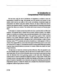
Adaption level and solution time comparison of DG quad-grid with Fluent quad-grid showing DG 2-level (top left) and 4-level (top right) and Fluent 2-level (bottom left) and 6-level (bottom right) ......................................................................
18
19
ACKNOWLEDGEMENTS Special thanks goes to Thomas Gessner and Christoph Hiemke from Fluent for assisting with the development of Fluent 6.1.11 and for providing solutions for the 7.62-mm problem. All CFD results presented in this report were created using EnSight produced by CEI.
111..
INTRODUCTION Tank cannon muzzle brakes are becoming a critical technology for future combat systems as recoil loads increase and system weight decreases. Muzzle brakes redirect forward momentum of the muzzle gases rearward to offset recoil load created by the cannon during firing. A deleterious effect of redirecting the muzzle gases rearward is high-pressure waves behind the cannon where operational personnel are located. Limitations are placed on blast overpressure due to physiological reasons, both to the body and ear of nearby troops. Experimental, full-scale testing of tank cannon systems is very expensive. As a result, simulation of the muzzle brake flow-field is highly desirable as an early design tool. Developing the specific techniques to model blast wave propagation of high-pressure, high-temperature gun propellant gases is critical to correctly simulate blast overpressure (refs 13). In order to do this, a validation case with sufficient quantitative and qualitative information about the very complex flow-field created by muzzle blast is necessary to properly validate computational fluid dynamics (CFD) techniques. A CFD analysis of the 7.62-mm NATO rifle G3 with a DM-41 round was selected because of the large quantity of public domain information about the flow-field in the form of shadowgraph images and analysis (ref 1). PROBLEM DESCRIPTION The blowdown or emptying of a gun barrel after the projectile leaves the barrel is similar to the free jet expansion process. Because of the high pressures typically seen in guns, pressure ratios range from 5 to 1000. As a result, the flow exiting the barrel is typical of highly underexpanded jet flow. The flow-field around the muzzle of a gun barrel can be complicated and include flow phenomena such as expansion waves, compression waves, shocks, shear layers, and blast waves at speeds up to Mach 7 to 10 (see Figure 1) (ref 3). As the flow exits the barrel at the muzzle and begins to expand around the sharp comer of the gun barrel, a Prandtl-Meyer expansion fan forms at the muzzle plane and spreads angularly away from the gun axis and then terminates at the free-shear jet boundary or contact surface of the muzzle flow. These expansion waves reflect off the jet boundary forming a series of weak compression waves that coalesce to form a barrel or intercepting shock. In addition, these waves can propagate into the flow-field toward the main blast wave (ref 1). Downstream of the muzzle, a Mach disk forms across which the flow decelerates from supersonic to subsonic velocities. The Mach disk and barrel shock enclose a volume known as the shock-bottle. Initially the Mach disk is constrained by a blast-wave front or primary shock moving at sonic speed. This constraining action can be seen as a deformation in the plume boundary (ref 1). Outside of the barrel shock, at the comers of the Mach disk, a turbulent vortex ring forms as the flow tries to move toward the blast wave, but is constrained. The outside edge of this turbulent vortex ring forms the plume boundary. The turbulent vortex ring is caused by the large difference in tangential velocity and turbulent shear layer near the jet boundary. Once the blast moves away from the muzzle, the flow from the muzzle is similar to an unrestrained free jet
expansion. At this point, the flow from the muzzle is similar to that exiting a rocket exhaust nozzle (ref 1). The rifle selected for this CFD validation is the 7.62-mm NATO G3 with a 400-mm barrel length shooting a standard DM-41 training round. This particular configuration has a blowdown characterized by two precursor shocks and the main propellant flow. A precursor shock is formed as the bullet begins to accelerate down the barrel, causing compression waves to be formed in front of the bullet as the air column in front of it accelerates. In addition, leakage of propellant gases past the bullet can cause the air column to accelerate. The compression waves caused by acceleration of the air column coalesce to form a "precursor" shock. Depending on the speed of the bullet and the length of time the bullet is in the barrel, a second precursor shock may form. The precursor flow emanating from the muzzle is easily visualized with shadowgraphs because the gas column contains mostly air as opposed to cloudy propellant gas. For this reason, it is easier to compare with CFD results. The pressure ratios for the two precursor shocks for the 7.62-mm NATO G3 are 6 for the first precursor and 15 for the second precursor. After the bullet exits from the barrel and uncorks the propellant gas column behind it, the flow of the main propellant gases begins. The main propellant flow is similar to the precursor flow, only with pressure ratio typically one to two orders-of-magnitude higher. The precursor contributes very little to the overall blast effect of the gun. The propellant gas exits the barrel at a pressure ratio of 660. Because the pressure is so much higher than the precursor wave, the main blast wave quickly overtakes the precursor blast wave. In addition, because of the large quantities of unburnt propellant and water vapor in the propellant gases, viewing the shock structure of the main propellant blast wave with shadowgraphs is very difficult. DISCONTINUOUS GALERKIN CODE BACKGROUND The Discontinuous Galerkin Method (DGM) was introduced by Reed and Hill in 1973 (ref 4). Recently, the method has become popular in solving fluid dynamic problems. The DGM is somewhere between a finite element and finite volume method. It allows double discretization or discretization of the geometrical computational domain (the grid), as well as the functional domain (flow equations). This allows one to adapt both the grid elements and the order of the flow equations. Adaption of the grid is typically referred to as h-refinement and adaption of the flow equations to different orders as p-refinement. Both refinement techniques combined can optimize the computational effort required for complex blast analysis problems (ref 5). The DGM also allows for more general mesh configurations such as nonconformal meshes and discontinuous functions at the edge of the elements. This greatly simplifies both hrefinement and p-refinement. The main advantage of being able to solve discontinuous functions when analyzing shock-dependent problems is that shock structures and shock sharpness can still be maintained, even with very low levels of h-refinement or grid adaption. This is not true with continuous-based solvers. Thus, h-refinement and p-refinement were performed using density as an error indicator (ref 5).
2
In addition to being able to perform h-refinement and p-refinement, DGM also can perform local time-stepping while using an explicit inviscid solver with explicit time-stepping to perform unsteady flow calculations such as blast. Local time-stepping is a means by which a local Courant-Friedrichs-Levy (CFL) criterion is applied to each cell and then these and similarsized cells are solved at the CFL number. For example, if one full-sized cell in the domain and one-half-sized cell in the domain have similar flow properties, then the CFL limited explicit time-step size should be one-half as large for the one-half-sized cell. In this instance, two iterations would be performed on the half-sized cell, while only one iteration would be performed on the full-sized cell with local time-stepping. This could then be extended to the entire computational space and thereby reduce the total number of iterations required. This method also allows one to set the flow time-step size, unlike a typical explicit solver. Explicit time-step flow solvers tend to be more efficient and time accurate for solving blast wave problems than implicit schemes. A shock limiter is used to limit pressure gradients near shocks to physical levels. These techniques have been incorporated into a CFD solver, referred to as the Discontinuous Galerkin Code (DG), being developed by the Scientific Computation Research Center, Rensselaer Polytechnic Institute. FLUENT BACKGROUND Fluent is a commercial CFD code that can perform solutions on various kinds of fluid dynamic problems. Recently, Fluent developed the capability to perform unsteady grid adaption (h-refinement) in a soon to be released version of the code, Fluent 6.1. A prerelease version of the code was used on the 7.62-mm NATO G3 problem in order to validate the unsteady grid adaption capability. The unsteady grid adaption capability within Fluent can perform nonconformal grid adaption. For this analysis, adaption was performed using density gradient as an error estimator. Solution refinement was limited by specifying a minimum cell size of 2.5e-8m 2 . This resulted in refinement levels of up to six for the analysis of the first precursor flow. The second-order inviscid solver was used to solve the explicit flow equations with an explicit time-stepping scheme. CFD SETUP AND BOUNDARY CONDITIONS The 7.62-mm NATO G3 rifle with a 400-mm barrel length shooting a standard DM-41 training round was modeled using a two-dimensional half-grid tri-mesh and two-dimensional half-grid quad-mesh shown in Figures 2 and 3, respectively. The grid was made using Gambit, a meshing tool produced by Fluent, Inc. The modeling of blast problems utilizing two-dimensional rather than axisymmetric boundary conditions presents a problem. Blast wave development is inherently a threedimensional problem. Blast wave strength appears to be much higher than it actually is when utilizing two-dimensional boundary conditions. This effect is accentuated the farther the blast wave is from the muzzle or source. The results presented in this report are limited to twodimensional because of a limitation in the DG solver to only run two-dimensional simulations and not axisymmetric.
3
A time-varying pressure inlet was used to control total pressure, static pressure, static temperature, and mass fraction of the air and K503 propellant (only Fluent modeled the change from air to K503; DG utilized air for all flows) at 12.5-mm upstream of the muzzle (see Figures 2 and 3). The experimental data used for the pressure inlet boundary condition are based upon the measured static muzzle pressure of the NATO rifle shown in Figure 4 below (ref 1). Modifications to the release times of the second precursor and main propellant were required to match shadowgraph results. The K503 propellant characteristics, along with the static pressure data, were then used to derive the other required parameters for the pressure inlet using unsteady compressible flow theory. Because of the lack of information about the initial boundary conditions, it is possible that computation errors could occur in the CFD results. The boundary conditions are defined in CFD flow time, t, where time t = 0.0 corresponds to the flow beginning 12.5-mm upstream of the muzzle for the first precursor. This time, t = 0.0, would correspond to a flow time from the experiment of texp = -400 jisec. The boundary conditions used for the unsteady pressure inlet are as follows: Gas Properties: Air: R = 287 N-m/kg-0 K y,= 1.4 Cp = 1006 N-m/kg-°K K503 (used for Fluent analysis only): y,= 1.3 Cp = 2000 N-m/kg-°K Initial Conditions: p = 101325 Pa V= 0.0 m/s T= 300'K p = p/RT Precursor1: @ t < 342.28 gsec p = 0.6 MPa V= 548.1 m/s T = 631.626'K p = pIRT
4
Precursor2: @ 342.28 < t < 399.2 psec p = 1.5 MPa V= 905.146 m/s T= 838.8°K p = pIRT Main PropellantFlow: @ t > 399.2 p.sec p=
101325*659.369e(-1" 484 "8*(t°°°°4°1 5 ) MPa
V = 905.146 m/s T= 1700'K p = pIRT It should be noted that the starting times for the second precursor and main propellant flows had to be adjusted relative to the starting times shown in Figure 4. This was necessary to get the CFD results to match the shadowgraph images properly. The inaccuracy in start time of these events is possibly due to inaccuracies in measurement times of the pressure at the 12.5-mm or due to improper specification of boundary conditions for the CFD problem. The exponential pressure equation for the main propellant flow shown above was not modified for the new main propellant start time. The solution was run using the unsteady explicit solver with explicit local time-stepping. However, the local time-step cannot be larger than 10 to 20 times as large as the minimum cell size CFL criterion. The CFL limit for each cell was limited to 0.3 to allow for curvature in flow properties within each cell to be resolved. The material properties of the species were modeled, including the specific heat at constant pressure and gas constant. A constant pressure, velocity, and density far-field boundary condition with values identical to the initial conditions were utilized. The far-field boundary is approximately 100 calibers from the muzzle with most of the flow-field phenomena being investigated occurring within 25 calibers of the muzzle. Muzzle blast typically consists of over-expanded nozzle flow interacting with blast wave shocks. To model these propagating shocks well, it is necessary to have fine grid near the shock front as it passes through the flow domain. To minimize solution time, nonconformal grid adaptation is utilized to adapt to density gradients. Various levels of adaption were investigated. For the solutions, various grid types and h-refinement levels were used, including a DG tri-mesh grid at 5-levels of adaption for solution times up to texp = -250 psec, an adapted DG quad-mesh grid at 4-levels of adaption for solution times past texp = -250 gsec, and a Fluent tri-mesh grid at 2.5e-8m 2 minimum cell size adaption level. Each of these grid types is shown in Figure 5 at t = 1.Oe-4 seconds. The mesh adaption was performed every other time-step for both the DG and Fluent analyses. The time-step for the Fluent analysis was dictated by the CFL = 0.5 criterion applied to the smallest cell in the flow domain. The time-step for DG 5-level tri-mesh was based
5
on a local time-step setting of 2.0e-7 seconds for the 5-level tri-mesh and 5.0e-7 seconds for the 4-level quad-mesh. For this particular study, only nonconformal h-refinement of the grid was performed for the DG code; p-refinement was not used for the DG simulations; and the polynomial order of the flow equations was fixed at first-order. For the Fluent simulations, the flow equations were fixed second-order. RESULTS The first precursor shock is created in the muzzle by the compression of the air in the gun tube by the accelerating bullet. This shock wave exits the barrel at approximately tex, = -400 gts before shot exit. Figures 6 through 15 present comparisons of shadowgraphs of experimental data (ref 1) and logarithmic density grayscale contour plots from 395 microseconds as the first precursor begins to exit the barrel until 120 microseconds after the main propellant flow begins. In the comparison figures, a logarithmic density grayscale contour plot of the CFD results was used to compare to experimental shadowgraph images. The shadowgraphs show curvature of density throughout the flow-field. By using a logarithmic scale for the CFD density contours, weak shock patterns such as the primary blast wave are more visible and easier to compare to experimental shadowgraph images. It should be noted that in some of the shadowgraph images a 50-mm ruler is placed on the barrel to provide a reference measurement. In addition, a collar on the end of the barrel is present. The ruler and collar were not modeled in the CFD simulation. As seen in Figure 6, at txp = -395 is, the exit of the first precursor shock wave is about the same distance from the gun tube with a similar thickness and shape for the DG simulation. In addition, the DG simulation shows the beginning of the vortical flow at the comers of the muzzle. This comer flow is not as visible in the shadowgraph image. This comer flow later develops into an expansion wave. In Figure 7, at texp = -370 gIs, the outer spherical shock of the first precursor has developed. The outer blast wave has a nearly identical shape and size for both the Fluent and DG simulations. In addition, the Mach disk is modeled, but is a slightly different shape than the experimental data. The barrel shock and free-shear layer are both modeled with the CFD simulation; however, the free-shear layer has a greater angle relative to the barrel and the barrel shock a lower angle. The barrel shock is just barely visible in the shadowgraph image. The outer free-shear layer is more visible in the shadowgraph image. In addition, the vortex ring is beginning to form showing a similar shape and size as the shadowgraph for both the Fluent and DG results. In the DG results, the free-shear layer shows disturbances propagating from the muzzle comer that are not present in the Fluent results or seen in the shadowgraph. This could be due to the discontinuous nature of the DG code to determine acoustic propagations.
6
In the Figure 8 shadowgraph, at tex, = -350 gIs, the shock bottle has now formed and is seen as formed by the edges of the barrel shock and the downstream Mach disk. In addition, more complex shock interactions occur. The beginning of the vortex at the comer of the shock bottle is beginning to form. The vortex formation is seen in both the DG and Fluent results. The DG results show more turbulence than the Fluent results. In addition, the waves propagating from the comer of the muzzle are more pronounced with DG. The inner barrel shock is visible in both DG and Fluent results. The outer blast wave is about the same size and distance from the muzzle with both DG and Fluent. The DG results also show waves propagating toward the rear edge of the blast wave. These waves are the result of the vortex formation. The plume boundary is also visible in the DG and Fluent results shown by a change from dark to light at the front of the Mach disk. The Figure 9 shadowgraph, at tex, = -250 gis, shows that the jet flow is fully developed and the typical shock diamond pattern of an over-expanded jet now exists. The over-expanded jet flow occurs because the outer shock boundary has propagated far enough from the main jet so that the muzzle flow expansion is uninhibited. The vortex flow at the comer of the Mach disk and free-shear layer are still present in the CFD images. The free-shear layer has a slightly higher angle in the CFD results and the barrel shock is not as sharp. Fluent shows the oblique shocks emanating downstream of the Mach disk more clearly than DG, however, both codes smear these shocks substantially. The plume boundary is visible with both codes. Once again, the waves propagating from the comer of the muzzle barrel are seen with DG and not with Fluent. In addition, DG shows waves propagating toward the rear blast wave. These waves can also be seen in the shadowgraph. In Figure 10, at tex, = -80 gis, the flow is more developed. For the rest of the results, there are no Fluent comparisons and a 4-level quad-grid was used for the DG solution. A courser initial grid and a lower level of refinement were used for the longer solution times due to the high CPU time required for these simulations. The DG shows substantially more shock structure. The oblique shocks emanating from the comer of the Mach disk not visible at tx),P 250 gis are now clearly visible. Either these shocks are delayed or they are obscured in the shadowgraph image by the high level of turbulence. The free-shear layer is also at a higher angle once again with the DG results. In addition, there is less turbulent structure in these results because of running an inviscid solution without a turbulence model, however, most of the largescale turbulence is still present. The plume appears to less elongated for DG. The DG also shows the blast waves emanating from the turbulent vortices that are not shown in the shadowgraph. The main blast wave for DG appears to be similar in shape to the shadowgraph, but possibly farther downstream from the gun tube. The waves propagating from the gun tube comer are smeared more, due to the lower level of grid resolution. Figure 11, at texp = -40 gts, shows the second precursor shock. The rear blast wave in the second precursor from the DG solution is similar to the shadowgraph image. The front of the precursor shows a shock wave in the DG solution that is not present in the shadowgraph. The first precursor plume is also slightly larger. The Mach disk from the first precursor is visible in the DG solution, as well as the oblique shocks emanating from the comer. These shocks can be seen inside the plume turbulence in the shadowgraph.
7
In Figure 12, at texp = -5 gIs, the flow main blast wave has begun to exit the gun barrel. Once again, the front of the main blast wave is much wider than the shadowgraph, as was the case for the second precursor. The second precursor has a similar shape and size as the shadowgraph, with the exception being the front of the precursor wave. The presence of the first precursor seems to have a strong effect on the second precursor in the DG results. It appears that there is more dissipation in the shadowgraph. This in part could be a result of the presence of significant turbulence. This turbulence is breaking up the shock structure. This breakup is not occurring with the DG results, and indicates the need for some turbulence modeling in the CFD. Figure 13, at t,,p = +35 ps, illustrates the main blast wave flow. Once again, turbulence has smeared a lot of the shock structure in the shadowgraph that is present in the DG results. In addition, the basic shape of the blast wave is distorted, both at the rear, and especially at the front. The shock angle for the free-shear layer is at a very high angle compared to the precursor flow. The angle is similar in both the shadowgraph and DG results. The core muzzle flow is shown as a dark spot on the shadowgraph and a light spot for the DG results. The barrel shock angle indicated by the edge of the bright area in the DG results and a sharp dark edge inside the core flow of the shadowgraph are at similar angles. These large differences could easily be attributed to the two-dimensional modeling of the flow rather than axisymmetric or threedimensional modeling. The two-dimensional effects seem to have a more pronounced effect at the higher-pressure ratios of the main propellant flow. In Figure 14, at texp = +60 gis, the main propellant flow has developed. The distortion of the front blast wave can be seen more readily in the DG results. This is most likely a result of mixing effects and turbulence in the main propellant flow. The rear blast wave from the main propellant flow is not as perpendicular to the barrel as the results of the precursor blast wave. This could be the result of the precursor and main blast wave interaction not being modeled properly, as well as errors in the boundary conditions. In Figure 15 at texp = +120 Ps, the bullet is clearly visible in the shadowgraph image. The bullet movement was not modeled in the DG results. The free-shear layer and barrel shock now show a much higher angle for the DG results than for the shadowgraph results. In addition, the forward shape of the blast wave is now more distorted with the DG results. The back edge of the blast wave cannot be seen in the shadowgraph image, but is shown in the DG results. This indicates that this wave propagation is being retarded for some reason. Figures 16 and 17 show pressure versus distance along the 135-degree radial line emanating from the muzzle at texp z -350 gs and texp
-250 [is for both the Fluent and DG results.
The peak pressure (referred to as peak overpressure in blast terminology) and distance from the muzzle blast wave are similar for both the Fluent and DG results, indicating similar time accuracy and ability to maintain shock strength at these flow times. The DG results show a sharper shock front than the Fluent results however. This becomes very important as flow solution time increases. Once this shock becomes less and less sharp, the peak overpressure starts to drop and the wave begins to dissipate. The DG results also show more noise on the rear side of the blast wave. This is a result of the disturbances that are propagating into the flow field being resolved by DG and not by Fluent. Also, for tep z -250 pgs, Fluent is predicting the wave front being farther from the muzzle than DG, but with a similar shape. The DG shows a negative
8
pressure in front of the blast wave that Fluent does not. Both codes model the negative pressure drop behind the blast wave. Table 1 shows a comparison between the shadowgraph and DG of the distance from the muzzle centerline to the forward edge and rear edge along the barrel of the blast wave. This is done in order to compare the time accuracy of DG to the experimental results. As can be seen, the forward blast wave propagates about 22% faster than the experimental results for DG when looking at the -250 and -80 pLs times. This could indicate a problem with the boundary conditions, as well as time accuracy of the code. When looking at Figure 17, the rear blast wave for Fluent is moving even faster than DG. This seems to indicate time accuracy with blast wave modeling may be difficult, especially if initial conditions are incorrect. Table 1. First Precursor Blast Wave Distance Comparison Distance Rear (Along Barrel) CFD (cal) -395 N/A -350 2.2 -250 6.8 -80 14.7 tep
(jis)
Distance Rear (Along Barrel) Shadowgraph (cal) N/A 2.1 Not Visible Not Visible
Distance Front Distance Front CFD Shadowgraph (cal) (cal) 0.4 4.2 10.7 20.7
0.5 3.0 8.7 16.9
COMPUTATION COMPARISON The DG and Fluent are compared to each other, as well as different levels of refinement. Comparison simulations were run on a 2.4 GHz Xeon Dual Processor Dell Precision 530 with 1.0 GB of memory running Linux. In each case, a single processor was utilized to perform a serial computation. Grid sizes and computation times are compared, as well as overall results. Figure 18 depicts a comparison of DG and Fluent at 2-levels and 4-levels of refinement at texp z -350 p[s. Computation times and final grid sizes are shown below each logarithmic density contour. In addition, the grid structure is overlaid on the contour plot for each result. All flow equation computations are inviscid calculations with first-order equations. The same initial quad-paved grid is utilized for all computations. Grid adaption in both cases was performed on density For the 2-level adaption case, Fluent and DG have similar computation times; however, Fluent utilizes about twice as many elements as DG. In addition, the shock structure is sharper with DG than with Fluent. For the 4-level adaption case, Fluent utilizes an order-of-magnitude more elements than DG and almost twice the computation time. It would appear that Fluent is about five times faster per element than DG for the 4-level case, where Fluent takes twice as long to perform calculations on about ten times as many grid elements. However, DG used far fewer cells than Fluent and half the computation time to
9
produce better results for the 4-level case. This would indicate that DG could produce better results with fewer grid elements than Fluent. Some of the difference in computation time between DG and Fluent can be attributed to the fact that DG is a research level code that has not been optimized. However, one would expect there to be more computational overhead with a discontinuous calculation like DG as compared to a standard solver like Fluent. When comparing the results, DG is capable of maintaining shock sharpness, regardless of refinement level. Even with a 2-level grid adaption, the outer blast wave is just as sharp with the 2-level grid as with the 4-level grid. When comparing Fluent 2-level and 4-level grid adaptions, the shock structure is markedly smeared with the 2-level adaption. This would seem to indicate that standard solvers such as Fluent require high levels of grid adaption to maintain shock strength in moving shock and blast problems. Discontinuous solvers such as DG do not require refining to maintain shock strength. This is a huge advantage of discontinuous solvers. One can get reasonable results even with rather course grids, thereby making simulations that are more difficult feasible. This is the case for full three-dimensional problems where one is trying to determine shock strength at long distances from the gun muzzle. CONCLUSIONS Several conclusions can be drawn from this study of CFD application to gun muzzle blast. These include: "* The 7.62-mm NATO G3 CFD precursor flow results matched shadowgraph results well; however, the main propellant flow did not match as well. "* Unsteady grid adaption (h-adaptivity) is a critical technology to modeling gun muzzle blast. "* It is possible to get good results from standard solvers with high levels of adaption. "* Discontinuous solvers can model blast with courser grid adaption than standard solvers. "* Discontinuous solvers can model blast better than standard solvers for a given level of refinement. "* Discontinuous solvers can potentially require longer solution time than standard solvers. "* When modeling blast waves, it is recommended that axisymmetric or threedimensional grids be used if possible rather than two-dimensional grids.
10
REFERENCES 1. Klingenberg, Gunter, and Heimerl, Joseph M., Gun Muzzle Blast and Flash, Progress in Astronautics and Aeronautics Series, Vol. 139, AIAA, Washington, DC, 1992 (Figures reprnted with permission). 2. Dillon, Robert, "A Method of Estimating Blast Envelope Duration," Proceedingsof the Ninth U.S. Army Symposium on Gun Dynamics, ARDEC Technical Report ARCCB-SP-99015, (E. Kathe, Ed.), Benet Laboratories, Watervliet, NY, November 1998. 3. Carofano, Garry C., "Blast Computation Using Harten's Total Variation Diminishing Scheme," Technical Report ARLCB-TR-84029, Benet Laboratories, Watervliet, NY, October 1984. 4. Reed, W., and Hill, T., "Triangular Mesh Methods for the Neutron Transport Equation," Technical Report LA-UR-73-479, Los Alamos Scientific Laboratory, 1973. 5. Remade, J.F., Flaherty, J.E., and Shephard, M.S., "An Adaptive Discontinuous Galerkin Technique with an Orthogonal Basis Applied to Compressible Flow Problems," SIAM Journalon Scientific Computing, 2002.
11
•-
FLOW SEPARATIO INTERCEPTING SHOCK CONTACT SURFACE
PRIMARY SHOCK PLUME BOUNDARY
CONTACT SURFACE OBLIQUE SHOCK MACH DISK
Figure 1. Muzzle flow characteristics.
Figure 2. Initial tri-grid.
12
Figure 3. Initial quad-grid. M41
M3
~ L . '51SS NORMAL DM 41 ROUND
800. 400. 200. ,< LAJ
MUZZLE EXIT PRESSURE (PRESSURE PORT 31 (M 3)
100
0..3
10
2
0.1
0.2
BEFORE to
0.4" 1.2 2.0 2.8 3.6
- I IAFTER
41.
5.2
6.0
TIME t -- m/s to OR SHOT EJECTION
Figure 4. Gun geometry and pressure ratio profile for position M3 (ref 1).
13
b Figure 5. Unstructured nonconformal DG 5-level tri-grid (left), DG 4-level quad-grid (middle), and 2.5e-8m 2 minimum cell size Fluent tri-grid at t I .Oe-4 sec.
Figure 6. Shadowgraph (ref 1) (left) and DG 5-level tri-grid adaption logarithmic density contour (right) at tp = -395 gs.
............
/
..........
..
.
,;;,
'
Figure 7. Shadowgraph (ref 1) (left), DG 5-level adaption logarithmic density contour (middle), and Fluent 2.5e-8m 2 cell volume limit adaption at tep z -370 ps.
14
Figure 9. Shadowgraph (ref 1) (left), DG 5-level adaption logarithmic density contour (middle), and Fluent 2.5e-Sm 2cell volume limit adaption at t•,,p -250 pts.
80. ~~~~Figure
adaptionloaihcdestcnou(mde) DG 5-level Shadowgraph (ref 1) (left),an at tex),,• -350 JiS. limit)aato cll tolume anlugrthients2ietm
''
~~~~Figure
15
DG 5-level (ref 1) (left),an 10. Shadowgraph
nor(mde)
adaptionloaihidest
p = -250 at t,,p olume (right)aat c ont s ity loarthi dlent.e 15
ts.
-40
is
Figure 11. Shadowgraph (ref 1) (left) and DG 4-level quad-grid adaption logarithmic density contour (right) at texp = -4 jis.
L. Figure 12. Shadowgraph (ref 1) (left) and DG 4-level quad-grid adaption logarithmic density contour (right) at txp = -5 gts.
+ 3
Figure 13. Shadowgraph (ref 1) (left) and DG 4-level quad-grid adaption logarithmic density contour (right) at te p = +35 jIs.
16
3I
ýj.
Figure 14. Shadowgraph (ref 1) (left) and DG 4-level quad-grid adaption logarithmic density contour (right) at txp =+60 gts.
Figure 15. Shadowgraph (ref1) (left) and DG 4-level quad-grid adaption logarithmic density contour (right) at texp = +120 gs.
17
16000 _
14000 12000
"
m
Fluent*:
--
10000
*
~8000
_
S60
00, 4000, 2000'
- . - ..
-
0
' .-------
-2000 -4000 0.5
0
1.5
1
2.5
2
3.5
3
4
Distance (calibers)
Figure 16. Comparison of Fluent and DG pressure versus distance along the 135-degree radial at te, z -350 gs. The 0-degree radial is the direction of fire and the center of rotation is at the muzzle.
.
-- -.. • DG
-0000
S6000 a.
4000 2000
U
0 -2000
0
1
2
3
4
5
6
7
8
9
Distance (calibers)
Figure 17. Comparison of Fluent and DG pressure versus distance along the 135-degree radial at texp -250 gs. The 0-degree radial is the direction of fire and the center of rotation is at the muzzle.
18
10
-N,,N.. = = •.. .,->'
N
,•i
N.,
DG 2-level 1482 Elements Solution time =6 minutes
DG 4-level 5289 Elements Solution time =108 minutes
Flen 2-level 31482 Elements -Solution time = 5 minutes
Flen 4-level 50,45 Elements Solution time = 196 minutes
quad-gri
showing D
-
l(tpeft)
uend4-level (o
ih)adFun
(bottom left) and 6-1evel (bottom right). Results are at t,n, z-350 pts.
19
-ee
,
NOMENCLATURE CFD
Computational fluid dynamics
CFL
Courant-Friedrichs-Levy criterion
Cp
Specific heat at constant pressure, N-m/kg-°K
DG
Discontinuous Galerkin Code
DGM
Discontinuous Galerkin Method
p
Static pressure, MPa
Pe
Gun muzzle exit pressure
poIJ
Free stream ambient pressure
R
Gas constant, N-m/kg-°K
,
Ratio of specific heats
t
CFD flow time, sec
te",
Experimental flow time, sec or psec
T
Static temperature, °K
V
Velocity, m/s
p
3 Density, kg/mr
20
TECHNICAL REPORT INTERNAL DISTRIBUTION LIST NO. OF COPIES TECHNICAL LIBRARY ATT'N: AMSTA-AR-CCB-O TECHNICAL PUBLICATIONS & EDITING SECTION ATTN: AMSTA-AR-CCB-O PRODUCTION PLANNING & CONTROL DIVISION ATTN: AMSTA-WV-ODP-Q, BLDG. 35
NOTE: PLEASE NOTIFY DIRECTOR, BENtT LABORATORIES, ATrN: AMSTA-AR-CCB-O OF ADDRESS CHANGES.
3
TECHNICAL REPORT EXTERNAL DISTRIBUTION LIST NO. OF COPIES DEFENSE TECHNICAL INFO CENTER ATTN: DTIC-OCA (ACQUISITIONS) 8725 JOHN J. KINGMAN ROAD STE 0944 FT. BELVOIR, VA 22060-6218 COMMANDER U.S. ARMY TACOM-ARDEC ATMN: AMSTA-AR-WEE, BLDG. 3022 AMSTA-AR-AET-O, BLDG. 183 AMSTA-AR-FSA, BLDG. 61 AMSTA-AR-FSX AMSTA-AR-FSA-M, BLDG. 61 SO AMSTA-AR-WEL-TL, BLDG. 59 PICATINNY ARSENAL, NJ 07806-5000 DIRECTOR U.S. ARMY RESEARCH LABORATORY ATTN: AMSRL-DD-T, BLDG. 305 ABERDEEN PROVING GROUND, MD 21005-5066 DIRECTOR U.S. ARMY RESEARCH LABORATORY ATTN: AMSRL-WM-MB (DR. B. BURNS) ABERDEEN PROVING GROUND, MD 21005-5066
2
1 1 1 1 1 2
1
I
CHIEF COMPOSITES & LIGHTWEIGHT STRUCTURES WEAPONS & MATLS RESEARCH DIRECT I U.S. ARMY RESEARCH LABORATORY ATTN: AMSRL-WM-MB (DR. BRUCE FINK) ABERDEEN PROVING GROUND, MD 21005-5066
NO. OF COPIES COMMANDER U.S. ARMY RESEARCH OFFICE ATI'N: TECHNICAL LIBRARIAN P.O. BOX 12211 4300 S. MIAMI BOULEVARD RESEARCH TRIANGLE PARK, NC 27709-2211 COMMANDER ROCK ISLAND ARSENAL ATTN: SIORI-SEM-L ROCK ISLAND, IL 61299-5001 COMMANDER U.S. ARMY TANK-AUTMV R&D COMMAND ATTN: AMSTA-DDL (TECH LIBRARY) WARREN, MI 48397-5000 COMMANDER U.S. MILITARY ACADEMY ATTN: DEPT OF CIVIL & MECH ENGR WEST POINT, NY 10966-1792 U.S. ARMY AVIATION AND MISSILE COM REDSTONE SCIENTIFIC INFO CENTER ATTN: AMSAM-RD-OB-R (DOCUMENTS) REDSTONE ARSENAL, AL 35898-5000 NATIONAL GROUND INTELLIGENCE CTR ATTIN: DRXST-SD 2055 BOULDERS ROAD CHARLOTITESVILLE, VA 22911-8318
NOTE: PLEASE NOTIFY COMMANDER, ARMAMENT RESEARCH, DEVELOPMENT, AND ENGINEERING CENTER, BENtT LABORATORIES, CCAC, U.S. ARMY TANK-AUTOMOTIVE AND ARMAMENTS COMMAND, AMSTA-AR-CCB-O, WATERVLIET, NY 12189-4050 OF ADDRESS CHANGES.
2