Jan 13, 2015 - January 14, 2015. Abstract. To obtain the initial ... NA] 13 Jan 2015 ..... with a distance of 13 points between each sensor. The third image ...
arXiv:1501.02946v1 [math.NA] 13 Jan 2015
Computational Realization of a Non-Equidistant Grid Sampling in Photoacoustics with a Non-Uniform FFT Julian Schmid1 , Thomas Glatz1 , Behrooz Zabihian2 , Mengyang Liu2 , Wolfgang Drexler2 , and Otmar Scherzer1,3 1
Computational Science Center, University of Vienna, Oskar-Morgenstern-Platz 1, 1090 Vienna, Austria 2 Center for Medical Physics and Biomedical Engineering, Medical University of Vienna, Waehringer Guertel 18-20, 1090 Vienna, Austria 3 Radon Institute of Computational and Applied Mathematics, Austrian Academy of Sciences, Altenberger Str. 69, 4040 Linz, Austria
January 14, 2015 Abstract To obtain the initial pressure from the collected data on a planar sensor arrangement in Photoacoustic tomography, there exists an exact analytic frequency domain reconstruction formula. An efficient realization of this ˘ Zs ´ Fourier transformula needs to cope with the evaluation of the dataˆ aA form on a non-equispaced mesh. In this paper, we use the non-uniform fast Fourier transform to handle this issue and show its feasibility in 3D experiments. This is done in comparison to the standard approach that uses polynomial interpolation. Moreover, we investigate the effect and the utility of flexible sensor location on the quality of photoacoustic image reconstruction. The computational realization is accomplished by the use of a multi-dimensional non-uniform fast Fourier algorithm, where non-uniform data sampling is performed both in frequency and spatial domain. We show that with appropriate sampling the imaging quality can be significantly improved. Reconstructions with synthetic and real data show the superiority of this method. Keywords: Image reconstruction, Photoacoustics, non-uniform FFT
1
Introduction
Photoacoustic tomography is an emerging imaging technique that combines the good contrast of optical absorption with the resolution of ultrasound images (see for instance [19]). In experiments an object is irradiated by a short-pulsed laser beam. Depending on the absorption properties of the material, some light
energy is absorbed and converted into heat. This leads to a thermoelastic expansion, which causes a pressure rise, resulting in an ultrasonic wave, called photoacoustic signal. The signal is detected by an array of ultrasound transducers outside the object. Using this signal the pressure distribution at the time of the laser excitation is reconstructed, offering a 3D image proportional to the amount of absorbed energy at each position. This is the imaging parameter of Photoacoustics. Common measurement setups rely on small ultrasound sensors, which are arranged uniformly along simple geometries, such as planes, spheres, or cylinders covering the specimen of interest (see for instance [21, 20, 22, 19, 1] below). For the planar arrangement of point-like detectors there exist several approaches for reconstruction, including numerical algorithms based on filtered backprojection formulas and time-reversal algorithms (see for instance [20, 11, 23, 24]). The suggested algorithm in the present work realizes a Fourier inversion formula (see (1) below) using the non-uniform fast Fourier transform (NUFFT). This method has been designed for evaluation of Fourier transforms at nonequispaced points in frequency domain, or non-equispaced data points in spatial, respectively temporal domain. The prior is called NER-NUFFT (nonequispaced range-non uniform FFT), whereas the latter is called NED-NUFFT (non-equispaced data-non uniform FFT). Both algorithms have been introduced in [7]. Both NUFFT methods haven proven to achieve high accuracy and simultaneously reach the computational efficiency of conventional FFT computations on regular grids [7]. This work investigates photoacoustic reconstructions from ultrasound signals recorded at non-equispaced positions on a planar surface. To the best of our knowledge, this is a novel research question in Photoacoustics, where the use of regular grids is the common choice. For the reconstruction we propose a novel combination of NED- and NER-NUFFT, which we call NEDNER-NUFFT, based on the following considerations: 1. The discretization of the analytic inversion formulas (see (1)) contains evaluation at non-equidistant sample points in frequency domain. 2. In addition, and this comes from the motivation of this paper, we consider evaluation at non-uniform sampling points. The first issue can be solved by a NER-NUFFT implementation: For 2D photoacoustic inversion with uniformly placed sensors on a measurement line such an implementation has been considered in [9]. This method was used for biological photoacoustic imaging in [15]. In both papers the imaging could be realized in 2D because integrating line detectors [4, 12] have been used for data recording. In this paper, however, the focus is on 3D imaging, because measurements are taken with point sensors. Experimentally, we show the applicability and superiority of the (NED)NER-NUFFT reconstruction formula in three spatial dimensions, compared with standard interpolation FFT reconstruction. To be precise, in this paper we conduct three dimensional imaging implemented using NEDNER-NUFFT, with ultrasound detectors aligned non-uniformly on a
measurement plane. To easily assess the effect of a given arrangement, also 2D numerical simulations have been conducted, to support the argumentation. We quantitatively compare the results with other computational imaging methods: As a reference we use the k-wave toolbox [17] with a standard FFT implementation of the inversion algorithm. The NEDNER-NUFFT yields an improvement of the lateral and axial resolution (the latter even by a factor two). The outline of this work is as follows: In Section 2 we outline the basics of the Fourier reconstruction approach by presenting the underlying Photoacoustic model. We state the Fourier domain reconstruction formula (1) in a continuous setting. Moreover, we figure out two options for its discretization. We point out the necessity of a fast and accurate algorithm for computing the occurring discrete Fourier transforms with nonuniform sampling points. In Section 3 we briefly explain the idea behind the NUFFT. We state the NER-NUFFT (subsection 3.1) and NED-NUFFT (subsection 3.2) formulas in the form we need it to realize the reconstruction on a non-equispaced grid. In Section 4 we discuss the 3D experimental setup. The NER-NUFFT is compared with conventional FFT reconstruction. A test chart is used to quantify resolution improvements in comparison to the k-wave FFT reconstruction with linear interpolation. In axial direction this improvement was about 170% while reducing the reconstruction time by roughly 35%. In Section 5 we then turn to the NEDNER-NUFFT in 2D with simulated data, in order to test different sensor arrangements in an easily controllable environment. An equiangular arrangement turns out to yield an improvement of over 40% compared to the best choice of equispaced sensor arrangement. Furthermore, we use the insights gained from the 2D simulations to develop an equi-steradian sensor arrangement for our 3D measurements. We apply our NEDNER-NUFFT approach on these data and quantitatively compare the outcomes with reconstructions from equispaced data obtained by the NER-NUFFT approach. Our results show a significant improvement of the already superior NER-NUFFT.
2
Numerical Realization of a Photoacoustic Inversion Formula
Let U ⊂ Rd be an open domain in Rd , and Γ a d − 1 dimensional hyperplane not intersecting U . Mathematically, photoacoustic imaging consists in solving the operator equation Q[f ] = p|Γ×(0,∞) , where f is a function with compact support in U and Q[f ] is the trace on Γ × (0, ∞) of the solution of the equation
∂tt p − ∆p = 0 in Rd × (0, ∞) , p(·, 0) = f (·) in Rd , ∂t p(·, 0) = 0 in Rd . In other words, the photoacoustic imaging problem consists in identifying the initial source f from measurement data g = p|Γ×(0,∞) . An explicit inversion formula for Q in terms of the Fourier transforms of f and g := Q[f ] has been found in [25]. Let (x, y) ∈ Rd−1 × R+ . Assume without loss of generality (by choice of proper basis) that Γ is the hyperplane described by y = 0. Then the reconstruction reads as follows: F[f ] (K) =
2Ky F[Qf ] (Kx , κ (K)) . κ (K)
(1)
where F denotes the d-dimensional Fourier transform: Z 1 F[f ] (K) := e−iK·(x,y) f (x)dx , (2π)n/2 Rd
and κ (K) = sign (Ky )
q
Kx2 + Ky2 ,
K = (Kx , Ky ) . Here, the variables x, Kx are in Rd−1 , whereas y, Ky ∈ R. For the numerical realization these three steps have to be realized in discrete form: We denote evaluations of a function ϕ at sampling points (xm , yn ) ∈ (−X/2, X/2)d−1 × (0, Y ) by ϕm,n := ϕ(xm , yn ) .
(2)
For convenience, we will modify this notation in case of evaluations on an equispaced Cartesian grid. We define the d-dimensional grid Gx × Gy := {−Nx /2, . . . , Nx /2 − 1}d−1 × {0, . . . , Ny − 1} , and assume our sampling points to be located on m∆x , n∆y , where (m, n) ∈ Gx × Gy , and write ϕm,n = ϕ(m∆x , n∆y ) ,
(3)
where ∆x := X/Nx resp. ∆y := Y /Ny are the occurring step sizes. In frequency domain, we have to sample symmetrically with respect to Ky . Therefore, we also introduce the interval GKy := {−Ny /2, . . . , Ny /2 − 1}.
Since we will have to deal with evaluations that are partially in-grid, partially not necessarily in-grid, we will also use combinations of (2) and (3). In this paper, we will make use of discretizations of the source function f , the data function g and their Fourier transforms fˆ resp. gˆ. Let in the following X d−1 fˆj,l = fm,n e−2πi(j·m+ln)/(Nx Ny ) (m,n)∈Gx ×Gy
denote the d-dimensional discrete Fourier transform with respect to space and time. By discretizing formula (1) via Riemann sums it follows 2l X −2πi κj,l n/Ny e fˆj,l ≈ κj,l n∈Gy
·
(4) d−1
X
e−2πi(j·m+ln)/Nx
gm,n ,
m ∈ Gx
where p κj,l = sign (l) j 2 + l2 , (j, l) ∈ Gx × GKy . This is the formula from [9]. Remark 1. Note that we use the interval notation for the integer multi-indices for notational convenience. Moreover, we also choose the length of the Fourier transforms to be equal to Nx in the first d − 1 dimensions, respectively. This could be generalised without changes in practice. Now, we assume to sample g at M , not necessarily uniform, points xm ∈ (−X/2, X/2)d−1 : Then, 2l X −2πiκj,l n/Ny fˆj,l ≈ e κj,l n∈Gy
·
M X m=1
(5) hm −2πi(j·xm )/M e gm,n . ∆xd−1
The term hm represents the area of the detector surface around xm and has to M P fulfil hm = (Nx ∆x )d−1 = X d−1 . Note that the original formula (4) can be m=1
received from (5) by choosing {xm } to contain all points on the grid ∆x Gx . Formula (5) can be interpreted as follows: Once we have computed the Fourier transform of the data and evaluated the Fourier transform at nonequidistant points with respect to the third coordinate, we obtain the (standard, equispaced) Fourier coefficients of f . The image can then be obtained by applying standard FFT techniques.
The straightforward evaluation of the sums on the right hand side of (5) would lead to a computational complexity of order Ny2 × M 2 . Usually this is improved by the use of FFT methods, which have the drawback that they need both the data and evaluation grid to be equispaced in each coordinate. This means that if we want to compute (5) efficiently, we have to interpolate both in domain- and frequency space. A simple way of doing that is by using polynomial interpolation. It is used for photoacoustic reconstruction purposes for instance in the k-wave toolbox for Matlab [17]. Unfortunately, this kind of interpolation seems to be sub-optimal for Fourier-interpolation with respect to both accuracy and computational costs [7, 25] A regularized inverse k-space interpolation has already been shown to yield better reconstruction results [10]. The superiority of applying the NUFFT, compared to linear interpolation, has been shown theoretically and computationally by [9].
3
The non-uniform fast Fourier transform
This section is devoted to the brief explanation of the theory and the applicability of the non-uniform Fourier transform, where we explain both the NERNUFFT (subsection 3.1) and the NED-NUFFT (subsection 3.2) in the form (and spatial dimensions) we utilise them afterwards. The NEDNER-NUFFT algorithm used for implementing (5) essentially (up to scaling factors) consists of the following steps: 1. Compute a d − 1 dimensional NED-NUFFT in the x-coordinates due to our detector placement. 2. Compute a one-dimensional NER-NUFFT in the Ky -coordinate as indicated by the reconstruction formula (5). 3. Compute an equispaced d-dim inverse FFT to obtain a d dimensional picture of the initial pressure distribution.
3.1
The non-equispaced range (NER-NUFFT) case
With the NER-NUFFT (non equispaced range – non-uniform FFT) it is possible to efficiently evaluate the discrete Fourier transform at non-equispaced positions in frequency domain. To this end, we introduce the one dimensional discrete Fourier transform, evaluated at non-equispaced grid points κl ∈ R: X ϕˆl = ϕn e−2πiκl n/N , l = 1, . . . , M. (6) n∈Gy
In order to find an efficient algorithm for evaluation of (6), we use a window function Ψ, an oversampling factor c > 1 and a parameter c < α < π(2c − 1) that satisfy:
1. Ψ is continuous inside some finite interval [−α, α] and has its support in this interval and 2. Ψ is positive in the interval [−π, π]. Then (see [7, 9]) we have the following representation for the Fourier modes occurring in (6): e−ixθ = √
X c ˆ − k/c)e−ikθ/c , |θ| ≤ π . Ψ(x 2πΨ(θ) k∈Z
(7)
ˆ are concentrated around 0. So we approximate By assumption, both Ψ and Ψ the sum over all k ∈ Z by the sum over the 2K integers k that are closest to κl + k. By choosing θ = 2πn/N − π and inserting (7) in (6), we obtain ϕˆl ≈
K X
ˆ l,k Ψ
X ϕn e−2πiln/cN , Ψn
n∈Gy
k=−K+1
(8)
l = 1, . . . , M . Here K denotes the interpolation length and Ψn := Ψ(2πn/Ny − π) , ˆ l,k := √c e−iπ(κl −(µl,k )) Ψ(κ ˆ l − (µl,k )) , Ψ 2π where µl,k is the nearest integer (i.e. the nearest equispaced grid point) to κl +k. The choice of Ψ is made in accordance with the assumptions above, so we need Ψ to have compact support. Furthermore, to make the approximation ˆ needs to be concentrated as much in (8) reasonable, its Fourier transform Ψ as possible in [−K, K]. In practice, a common choice for Ψ is the KaiserBessel function, which fulfils the needed conditions, and its Fourier transform is analytically computable.
3.2
The non-equispaced data (NED-NUFFT) case
A second major aim of the present work is to handle data measured at nonequispaced acquisition points xm in an efficient and accurate way. Therefore we introduce the non-equispaced data, d − 1 dimensional DFT ϕˆj =
M X
ϕm e−2πi(j·xm )/N ,
m=1
(9)
j ∈ Gx . The theory for the NED-NUFFT is largely analogous to the NER-NUFFT [7] as described in Subsection 3.1. The representation (7) is here used for each entry
of j and inserted (with now setting θ = 2πn/N ) into formula (9), which leads to ϕˆj ≈
M 1 X Ψj m=1
X
ˆ j,k ϕm Ψ
k∈{−K,...,K−1}d−1
(10)
· e−2πi(j·µm,k )/cM , where the entries in µm,k are the nearest integers to xm + k. Here we have used the abbreviations Ψj,k :=
d−1 Y
Ψ(2πj/Nx ) ,
i=1
ˆ j,k := Ψ
d−1 Y� i=1
c √ 2π
�
ˆ Ψ((x m )i − (µm,k )i ) ,
ˆ for the needed evaluations of Ψ and Ψ. Further remarks on the implementation of the NED- and NER-NUFFT, as well as a summery about the properties of the Kaiser-Bessel function and its Fourier transform can be found in [7, 9].
4
Comparison of NER-NUFFT and k-wave FFT
Before we turn to the evaluation of the algorithm we describe the photoacoustic setup. Our device consists of a FP (Fabry P´erot) polymer film sensor for interrogation [2, 3]. A 50 Hz pulsed laser source and a subsequent optical parametric oscillator (OPO) provide optical pulses. These pulses have a very narrow bandwidth and can be tuned within the visible and near infrared spectrum. The optical pulses are then transmitted via an optical fibre. When the light is emitted it diverges and impinges upon a sample with homogeneous fluence, thus generating a photoacoustic signal. This signal is then recorded via the FPsensor head. The sensor head consists of an approximately 38 µm thick polymer (Parylene C) which is sandwiched between two dichroic dielectric coatings. These dichroic mirrors have a noteworthy transmission characteristic. Light from 600 to 1200 nm can pass the mirrors largely unabated, whereas the reflectivity from 1500 to 1650 nm (sensor interrogation band) is about 95% [27]. The incident photoacoustic wave produces a linear change in the optical thickness of the polymer film. A focused continuous wave laser, operating within the interrogation band, can now determine the change of thickness at the interrogation point via FP-interferometry. We choose two 2D targets for comparison, a star and a USAF (US Air Force) resolution test chart. Both targets are made of glass with a vacuum-deposited durable chromium coating. The star target has 72 sectors on a pattern diameter of 5 mm, with an unresolved core diameter of 100 µm.
x [mm]
x [mm]
y [mm]
0 0
1
2
4 0
3
1
2
FFT
3
4
NUFFT
frequency [lp/mm]
1 2
NUFFT
3
FFT
4
frequency [lp/mm] intensity [a.u.] (max=10)
10
top
left
bottom
right
8 6 4 2 10
8 6 4 2
0
0.5
1
1.5
x [mm]
2
0
0.5
1
1.5
y [mm]
2
Figure 1: Segment of the MIP (maximum intensity projection) in the z-axis of a star sample, reconstructed using FFT and linear interpolation (top left) and using the NUFFT (top right) with a square plotted around the center. The intensity of the reconstructed image along the sidelines of the square is plotted, for both reconstructions. The purple line indicates the frequency of the star sample. The targets are positioned in parallel to the sensor surface at a distance of about 4 mm, and water is used as coupling medium between the target and the sensor. The interpolation length for the NER-NUFFT reconstruction is K = 6. The computational times are shown in Tab. 1 showing that the linearly interpolated FFT is about 30 % slower than the NER-NUFFT. A segment of the reconstructed star target is shown in Fig. 1. The intensity is plotted against the sides of an imaginary square (2.67 mm) placed around the center of the star phantom. It is clearly visible, that the FFT reconstruction is not able to represent the line pairs, when the density exceeds 10 lp/mm, corresponding to a resolution of 100 µm, whereas they are still largely visible for the NER-NUFFT reconstruction. For a quantitative comparison of the resolution we use the USAF chart. It is recorded on an area of 146×146 sensor points corresponding to 1.022×1.022 cm2 with a grid spacing of 70 µm and a time resolution of 8 ns. As yet there is no standardized procedure to measure the resolution of a photoacoustic imaging
Table 1: Comparison between the NED-NUFFT and FFT reconstruction for a USAF-chart and a comparison of computational times for both phantoms. The improvement in percent was caluclated by: 100 × (1 − FFT/NUFFT)
FWHM axial LSF FWHM lateral LSF Time: Star target Time: USAF chart
NUFFT 23.23 ± 0.56 µm 33.44 ± 7.95 µm 140 s 298 s
FFT 62.34 ± 0.62 µm 40.82 ± 7.34 µm 189 s 384 s
Improvement 168.47 ± 6.88 % 18.63 ± 8.50 % 35 % 29 %
system. We proceed similar to [27], by fitting a line spread function (LSF) and an edge spread function (ESF) to the intensities of our reconstructed data. For the LSF to be meaningful, its source has to approximate a spatial delta function. This is the case in the z-axis, since the chrome coating of the USAF target is just about 0.1 µm thick. We fit a Cauchy-Lorentz distribution to the z-axis of our reconstructed data for 49 adjacent xy-coordinates. Their positions are marked as a black square within the white square, depicted in the bottom images of Fig. 2. The reconstruction in the z-axis for a single point is shown in the bottom right inlay of Fig. 2, for 8 points, covering a distance of 94.74 µm in the z-direction, around the maximum intensity. A fit of the Lorentz distribution is shown for both reconstruction methods. The FWHM (full width, have maximum) of the Lorentz distribution, 2a0 w I(z) = , π (w2 + 4(z − z0 )2 ) is the parameter w. The output I(z) is the intensity in dependence from the z-axis, and z0 and a0 are fitting parameters. The average and standard deviation of w for both of the 49 datasets are shown in Table 1. The line spread function FWHM of the FFT-reconstruction turns out to be more than twice as big as the one of the NER-NUFFT reconstruction. For the lateral resolution, there is no target approximating a delta function, so we have to use the ESF instead: � � � � 1 x − x0 1 I(x) = I0+ a0 arctan + . π w/2 2 The w here is the FWHM of the associated LSF, and I0 , x0 and a0 are fitting parameters. The ESF requires a step function as source, of which our target provides plenty. We choose the long side of 12 bars, marked by white lines in the bottom images of Fig. 2, for this fit. The data for a particular line is shown in the bottom left inlay. We omitted all datasets, where only one point marked the transition from low to high intensity, rendering the edge fit unreliable and resulting in unrealistic improvements of our new method well
MIPxy - FFT
11 mm
MIPxy - NER NUFFT
y
y x
z
11 mm
x
z
0.1 mm
z-axis vs. intensity ESF NUFFT intensity FFT intensity NUFFT fit FFT fit
10 µm
LSF
z-axis
Figure 2: Segment of the xy-MIP of an USAF chart reconstruction conducted with FFT (left) and NER-NUFFT (right). On the bottom images the data-sets used for the quantitative resolution are marked. The black square depicts the 49 xy-coordinates used for the LSF fit along the z-axis for the axial resolution. The data for a single point is shown in the bottom right inlay. The white lines show the intensity fit for the lateral resolution. The bottom left inlay shows the data for a single white line.
over 100%. Finally we averaged over 15 edges. The results are shown in Table 1. While the deviation between different edges is quite high, the improvement of our NER-NUFFT reconstruction for the 15 evaluated edges ranged from 6 to 44%.
5
Non-equidistant grid sampling
The current setups allow data acquisition at just one single sensor point for each laser pulse excitation. Since our laser is operating at 50 Hz data recording of a typical sample requires several minutes. Reducing this acquisition time is a crucial step in advancing Photoacoustics towards clinical and preclinical application. Therefore, in this work we try to maximize the image quality for a given number of acquisition points. We are able to do this, because our newly implemented NEDNER-NUFFT is ideal for dealing with non-equispaced positioned sensors. This newly gained flexibility of sensor positioning offers many possibilities to enhance the image quality, compared against a rectangular grid. For instance a hexagonal grid was found to yield an efficiency of 90.8 % compared with 78.5 % for an exact reconstruction of a wave-number limited function [13]. Also any non-equispaced grids that may arrive from a specific experimental setup can be efficiently computed via the NEDNER-NUFFT approach. Here, we will use it to tackle the limited view problem. Many papers deal with the limited view problem, when reconstructing images [6, 26, 16]. Our approach to deal with this problem is different. It takes into account that in many cases the limiting factor is the number of sensor points and the limited view largely a consequence of this limitation. In our approach we therefore use a grid arrangement that is dense close to a center of interest and becomes sparser the further away the sampling points are located. We realize this by means of an equiangular, or equi-steradian sensor arrangement, where for a given point of interest each unit angle or steradian gets assigned one sensor point. To understand the limited view problem, it is helpful to define a detection region. According to [26], this is the region which is enclosed by the normal lines from the edges of the sensor. Pressure waves always travel in the direction of the normal vector of the boundary of the expanding object. Therefore certain boundaries are invisible to the detector as depicted in Fig. 3.
5.1
Equiangular and equi-steradian projection sensor mask
For the equiangular sensor arrangement a point of interest is chosen. Each line, connecting a sensor point with the point of interest, encloses a fixed angle to its adjacent line. In that sense we mimic a circular sensor array on a straight line. The position of the sensor points can be seen on top of the third image in Fig. 4.
sensor
detection region
Figure 3: Depiction of the limited view problem. Edges whose normal vector cannot intersect with the sensor surface are invisible to the sensor. The invisible edges are the coarsely dotted lines. The detection region is marked by a grey background. The finely dotted lines are used to construct the invisible edges. Edges perpendicular to the sensor surface are always invisible for a plane sensor.
The obvious expansion of an equiangular projection to 3D is an equi-steradian projection. This problem is analogous to the problem of placing equispaced points on a 3D sphere and then projecting the points, from the center of the sphere, through the points, onto a 2D plane outside the sphere. We developed an algorithm for this problem, which is explained in detail in Appendix 9. Our input variables are the grid size, the distance of the center of interest from the sensor plane and the desired number of acquisition points, which will be rounded to the next convenient value. A sensor arrangement with 1625 points on a 226 × 226 grid is shown in the top left image in Fig. 7.
5.2
Weighting term
To determine the weighting term hm in Eq. 5 for 3D we introduce a function that describes the density of equidistant points per unit area ρp . In our specific case, ρp describes the density on a sphere around a center of interest. Further we assume that ρp is spherically symmetric and decreases quadratically with the distance from the center of interest r: ρp,s ∝ 1/r2 . We now define ρp,m for a plane positioned at distance r0 from the center of interest. In this case ρp,s (r) attenuates by a factor of sin α, where α = arcsin(r0 /r) is the angle of incidence. Hence ρp,m ∝ r0 /r3 . By applying the spacing of the regular grid . This yields a weighting term of: hm (r) ∝ r3 Analogously we can derive hm for 2D: hm (r) ∝ r2 We applied a normalization after the reconstruction to all measurements.
50 100 150 200
orginal
250 50
best equispaced NER-NUFFT reconstruction
100
y [points]
150 200 250 50 100
equiangular NED-NER-NUFFT reconstruction
150 200 250 50
nearestneighbour interpolation FFT reconstruction
100 150 200 250
100
200
300
400
500
600
700
800
900
1000
x [points]
Figure 4: Various reconstructions of a tree phantom (top) with different sensor arrangements. All sensor arrangements are confined to 32 sensor points. The sensor positions are indicated as white rectangles on the top of the images. The second image shows the best (see Fig.5) equispaced sensor arrangement, with a distance of 13 points between each sensor. The third image shows the NEDNER-NUFFT reconstruction with equiangular arranged sensor positions. The bottom image shows the same sensor arrangement, but all omitted sensor points are linearly interpolated and afterwards a NER-NUFFT reconstruction was conducted. For the application of this method to the FP setup it is noteworthy that there is a frequency dependency on sensitivity which itself depends on the angle of incidence, which has been extensively discussed in [5]. The angle of incidence for our specific setup is 62◦ . At this angle, the frequency components around 2 MHz get attenuated by more than 10 dB. Below 1 MHz the frequency response remains quite stable (attenuation below 5 dB) for the measurement angles occurring in our setup.
6
Computational assessment of different nonequispaced grid arrangements in two dimensions to tackle the limited view problem
A tree phantom, designed by Brian Hurshman and licensed under CC BY 3.01 , is chosen for the 2 dimensional computational experiments on a grid with x = 1024 z = 256 points. A forward simulation is conducted via k-wave [17]. The forward simulation of the k-wave toolbox is based on a first order k-space model. A PML (perfectly matched layer) of 64 gridpoints is added, as well as 30 dB of noise. In Fig. 4 our computational phantom is shown at the top. For each reconstruction a subset of 32 out of the 1024 possible sensor positions was chosen. In Fig. 4 their positions are marked at the top of each reconstructed image. For the equispaced sensor arrangements, we let the distance between two adjacent sensor points sweep from 1 to 32. The sensor points where always centered in the x-axis. To compare the different reconstruction methods we used the correlation coefficient and the Tenenbaum sharpness. These quality measures are explained in Appendix 10. We applied the correlation coefficient only within the region of interest marked by the white circle in Fig. 4. The Tenenbaum sharpness was calculated on the smallest rectangle, containing all pixels within the circle. The results are shown in Fig. 5. The Tenenbaum sharpness for the equiangular sensor placement was 23001, which is above all values for the equispaced arrangements. The correlation coefficient was 0.913 compared to 0.849, for the best equispaced arrangement. In other words, the equiangular arrangement is 42.3 % closer to a full correlation, than any equispaced grid. In Fig. 4 the competing reconstructions are compared. While the crown of the tree is depicted quite well for the equispaced reconstruction, the trunk of the tree is barely visible. This is due to the limited view problem. When the equispaced interval increases, the tree becomes visible, but at the cost of the crown’s quality. In the equiangular arrangement a trade off between these two effects is achieved. Additionally the weighting term for the outmost sensors is 17 times the weighting term for the sensor point closest to the middle. This amplifies the occurrence of artefacts, particularly outside of our region of interest. The bottom image in Fig. 4 shows the equiangular sensor arrangement, reconstructed in a conventional manner. The missing sensor points are interpolated to an equispaced grid, and a NER-NUFFT reconstruction is applied afterwards. We conducted a linear interpolation from our subset to all 1024 sensor points. The correlation coefficient for this outcome was 0.7348 while the sharpness measure was 21474. This outcome exemplifies the clear superiority of the NUFFT to conventional FFT reconstruction when dealing with non-equispaced grids. 1 http://thenounproject.com/term/tree/16622/
3
x105
1
2 0.5 1
Tenenbaum sharpness correlation coefficient 0
0
4
9
14
19
24
29
correlation coefficient
Tenenbaum sharpness
equiangular projection
0 34
intervall between two adjacent sensor points
Figure 5: Correlation coefficient and Tenenbaum sharpness for equispaced sensor arrangements with intervals between the sensor points reaching from 1 to 32. The maximum of the correlation coefficient is at 13. The corresponding reconstruction is shown in Fig. 4. The straight lines indicate the results for the equiangular projection.
7
3D application of the NED-NER-NUFFT with real data
For a qualitative assessment of our new sensor arrangement we need a 3D phantom. We choose a yarn which we record on a rectangular grid with 226 × 226 = 51076 sensor points, with a grid spacing of 60 µm and time sampling of dt = 8 ns. Hence an area of 13.56 × 13.56 mm is covered. As coupling medium water is used, in which the yarn is fully immersed. To determine the utility of non-equispaced grid sampling, we follow a certain routine. First we acquire a densely sampled dataset. Then we use a very small subset of the initially collected sensor data, to test different sensor arrangements. Therefore we can always use the complete reconstruction as our model standard together with the quality measurements explained in Appendix 10. An upsampling factor of 2 was used for all reconstructions, hence the reconstructed image of the MIP for the xy plane consists of 452 × 452 pixels. The complete reconstruction with the NER-NUFFT took 154 seconds. Maximum intensity projections (MIP) of this full reconstruction for all axis are shown in Fig. 6. The MIP in the xy plane is our model standard, for comparison with the other reconstructions. For the equi-steradian sensor mask we choose our center of interest right in the center of the xy-MIP where the little knot can be seen, 3.6 mm off the sensor surface. The resulting sensor mask, including the reconstruction is shown in Fig. 7, it consists of 1625 sensor points (or 3.18 % of the initial number of
2
distance [mm] 4 6 8
10
12
2
4
6
2 4 6 8 10 12
center of interest y x
y z
x 2
z
4 6
Figure 6: MIPs of all 3 planes for the NER-NUFFT reconstruction of a yarn phantom. sensor points). The weighting term, accounting for sensor sparsity is 9.7 times higher for the outermost sensor point, than for centermost sensor points in the xy-plane. The reconstruction for this arrangement took 134 seconds. We compared this arrangement to rectangular grids, which all had 41 × 41 = 1681 sensor points (or 3.29 % of the initial number of sensor points) but varying distances between two adjacent points. The grid with an interval between sensor points of 5 is shown on the top left in Fig. 7. In Fig. 8 the equi-steradian grid is compared with 2 equispaced grids. To get a more precise measure of the correlation between the reconstructed images and the model standard, we calculated the correlation coefficient only within a region of interest. The region of interest is firstly confined by a centered disc, whose boundary is shown as a dotted circle in the inlay in Fig. 8. The x-axis shows the number of pixels of interest used to calculate the correlation coefficient within this disc. These pixels are increased according to the intensity of the corresponding pixels of the model’s standard MIP. Fig. 8 demonstrates that the correlation coefficient for the equi-steradian arrangement, always remains better, within the depicted disc, when competing against the two strongest equispaced grids. In Fig. 9 the 4 equispaced arrangements, with intervals reaching from 2 to 5 are compared to the equi-steradian grid. Here the pixels of interest are set to a threshold of at least 4% of the maximum value, while the diameter is increased. The dotted straight lines indicate the side length of the square of a particular
3 mm
3 mm
Figure 7: The sensor placement for the cirular arrangement is shown on the top left image, comprising 1625 sensor points. On the top right an equispaced sensor arrangement with 41×41 = 1689 sensor points is displayed. The intervall between two adjacent sensor points is 5 for this configuration. The bottom images show MIPs of the NED-NER-NUFFT reconstruction only using the sensor points shown above. 1
increasing number of points within mask
0.98
correlation coefficient
0.96 0.94 fixed diameter for mask 0.92 0.9 MIP for equi steradian grid MIP equispaced: intervall 4 MIP equispaced: intervall 5
0.88 0.86
0
10.000 20.000 30.000 40.000 50.000 pixels used for correlation coefficient calculation
60.000
Figure 8: Correlation coefficient calculated on different number of pixels, for 3 different reconstructed MIPs. Pixels of interest are added according to the intensity of the corresponding pixels of the model standard image (Fig. 6). In the inlay the correlation coefficient mask is shown for 20087 points which corresponds to all pixels with at least 4% of the maximum value of the model standard and is the value used in Fig. 9.
1
correlation coefficient a.u.
0.95
x
x 0.9
0.85
0.8
x 0.75
x
x
2
MIP: equi steradian grid MIP: equispaced- intervall 2 MIP: equispaced- intervall 3 MIP: equispaced- intervall 4 MIP: equispaced- intervall 5 sidelength of sensor square 4
6 8 10 diameter of region of interest [mm]
12
Figure 9: Correlation Coefficient calculated on pixels of interest with at least 4% of the maximum value of the model standard, for an increasing diameter of the confining disc. The straight line at 8.4 mm corresponds to the straight line in Fig. 8. The other straight lines indicate the side length of the square of a particular equispaced sensor point arrangement. equispaced sensor point arrangement. As expected the correlation coefficient for this equispaced sensor arrangement starts to decline around that threshold. The correlation coefficient for the equi-steradian grid starts to fall behind the equispaced grid of interval 5 towards the end. This is expected, since the equi-steradian grid is only meant to give better results for a region of interest around the center. This is very clearly the case. Between a diameter of 2 to 8 mm the correlation coefficient is on average 25.14 % closer to a value of 1 than its strongest equispaced contender of interval 4, and 30.87 % better than the interval 5 grid. At a diameter of 7.2 mm the correlation coefficient for the equi-steradian grid was 0.960 compared to 0.947 for the interval 4 grid and 0.944 for the interval 5 grid. This is 24.8 % and 28.6% closer to full correlation. Fig. 10 shows the normalized Tenenbaum sharpness. The Tenenbaum sharpness, unlike the correlation coefficient, cannot be calculated on non-adjacent grid points, therefore it has been calculated on the smallest rectangle, that contains all pixels of interest. The equi-steradian has the highest sharpness for most values, with the interval 4 grid being very slightly better around a diameter of 3-4 mm. There is a drop of the Tenenbaum sharpness towards the end.
8
Discussion and Conclusion
We computationally implemented a 3D non-uniform FFT photoacoustic image reconstruction, called NER-NUFFT (non equispaced range-non uniform FFT) to efficiently deal with the non-equispaced Fourier transform evaluations arising in the reconstruction formula. This method was compared with the k-wave
normalized Tenenbaum sharpness
1 MIP: equi steradian grid MIP: equispaced - intervall 2 MIP: equispaced - intervall 3 MIP: equispaced - intervall 4 MIP: equispaced - intervall 5
0.8 0.6 0.4 0.2 0
2
4
6 8 10 diameter of region of interest [mm]
12
Figure 10: Tenenbaum Sharpness calculated on pixels of interest with at least 4% of the maximum value of the model standard. The Tenenbaum sharpness is calculated on the smallest rectangle, that contains all pixels of interest. implemented FFT reconstruction, which uses a polynomial interpolation. The two reconstruction methods where compared using 2D targets. The lateral resolution showed an improvement of 18.63 ± 8.5% which is in good agreement with the illustrative results for the star target. The axial resolution showed an improvement of 168.47 ± 6.88%. The computation time was about 30% less, for the NER-NUFFT than the linearly interpolated FFT reconstruction. In conclusion the NER-NUFFT reconstruction proved to be unequivocally superior to conventional linear interpolation FFT reconstruction methods. We further implemented the NED-NER-NUFFT (non equispaced data-NERNUFFT), which allowed us to efficiently reconstruct from data recorded at nonequispaced placed sensor points. This newly gained flexibility was used to tackle the limited view problem, by placing sensors more sparsely further away from the center of interest. We developed an equiangular sensor placement for 2D and an equi-steradian placement in 3D, which assigns one sensor point to each angle/steradian for a given center of interest. In the 2D computational simulations we showed that this arrangement significantly enhances image quality in comparison to regular grids. In 3D we conducted experiments, where a yarn phantom was recorded. The maximum intensity projection (MIP) of the full reconstruction was compared to MIPs of reconstructions that only used about 3% of the original data. Within our region of interest, the correlation of our image was 0.96, which is 24.8% closer to full correlation than the best equispaced arrangement, reconstructed from slightly more sensor points. The sensor placement to tackle the limited view problem, combined with the NED-NER-NUFFT gives significantly better results for an object located at the center of a bigger sensor surface. This result was confirmed in the 2D simulation as well as for real data in 3D.
Acknowledgment This work is supported by the Medical University of Vienna, the European projects FAMOS (FP7 ICT 317744) and FUN OCT (FP7 HEALTH 201880), Macular Vision Research Foundation (MVRF, USA), Austrian Science Fund (FWF), Project P26687-N25 (Interdisciplinary Coupled Physics Imaging), and the Christian Doppler Society (Christian Doppler Laboratory ”Laser development and their application in medicine”).
References [1] P. Beard. Biomedical photoacoustic imaging. Interface Focus, 1:602–631, 2011. [2] P.C. Beard. Two-dimensional ultrasound receive array using an angle-tuned fabry-perot polymer film sensor for transducer field characterization and transmission ultrasound imaging. IEEE Trans. Ultrason., Ferroeletr., Freq. Control, 52(6):1002–1012, June 2005. [3] P.C. Beard, F. Perennes, and T.N. Mills. Transduction mechanisms of the fabry-perot polymer film sensing concept for wideband ultrasound detection. IEEE Trans. Ultrason., Ferroeletr., Freq. Control, 46(6):1575–1582, November 1999. [4] P. Burgholzer, C. Hofer, G. Paltauf, M. Haltmeier, and O. Scherzer. Thermoacoustic tomography with integrating area and line detectors. IEEE Trans. Ultrason., Ferroeletr., Freq. Control, 52(9):1577–1583, September 2005. [5] B.T. Cox and P.C. Beard. The frequency-dependent directivity of a planar fabry-perot polymer film ultrasound sensor. IEEE Trans. Ultrason., Ferroeletr., Freq. Control, 54(2):394–404, 2007. [6] W. Dan, C. Tao, X.-J. Liu, and X.-D. Wang. Influence of limited-view scanning on depth imaging of photoacoustic tomography. Chinese Physics B, 21(1):014301, 2012. [7] K. Fourmont. Non-equispaced fast Fourier transforms with applications to tomography. J. Fourier Anal. Appl., 9(5):431–450, 2003. [8] F. C. A. Groen, I. T. Young, and G. Ligthart. A comparison of different focus functions for use in autofocus algorithms. Cytometry, 6(2):81–91, 1985. [9] M. Haltmeier, O. Scherzer, and G. Zangerl. A reconstruction algorithm for photoacoustic imaging based on the nonuniform FFT. IEEE Trans. Med. Imag., 28(11):1727–1735, November 2009.
[10] M. Jaeger, S. Sch¨ upbach, A. Gertsch, M. Kitz, and M. Frenz. Fourier reconstruction in optoacoustic imaging using truncated regularized inverse k-space interpolation. Inverse Probl., 23:S51–S63, 2007. [11] P. Kuchment and L. Kunyansky. Mathematics of thermoacoustic tomography. European J. Appl. Math., 19:191–224, 2008. [12] G. Paltauf, R. Nuster, M. Haltmeier, and P. Burgholzer. Photoacoustic tomography with integrating area and line detectors. In L. V. Wang, editor, Photoacoustic Imaging and Spectroscopy, Optical Science and Engineering, pages 251–263. CRC Press, Boca Raton, FL, 2009. [13] D. P. Petersen and D. Middleton. Sampling and reconstruction of wavenumber-limited functions in N -dimensional Euclidean spaces. Inform.and Control, 5:279–323, 1962. [14] O. Scherzer, editor. Handbook of Mathematical Methods in Imaging. Springer, New York, 2011. [15] R. Schulze, G. Zangerl, M. Holotta, D. Meyer, F. Handle, R. Nuster, G. Paltauf, and O. Scherzer. On the use of frequency-domain reconstruction algorithms for photoacoustic imaging. J. Biomed. Opt., 16(8):086002, 2011. Funded by the Austrian Science Fund (FWF) within the FSP S105 - “Photoacoustic Imaging”. [16] C. Tao and X. Liu. Reconstruction of high quality photoacoustic tomography with a limited-view scanning. Opt. Express, 18(3):2760–2766, Feb 2010. [17] B. E. Treeby and B. T. Cox. K-Wave: MATLAB toolbox for the simulation and reconstruction of photoacoustic wace fields. J. Biomed. Opt., 15:021314, 2010. [18] B. E. Treeby, T. K. Varslot, E. Z. Zhang, J. G. Laufer, and P. C. Beard. Automatic sound speed selection in photoacoustic image reconstruction using an autofocus approach. Biomed. Opt. Express, 16(9):090501–090501–3, 2011. [19] L. V. Wang, editor. Photoacoustic Imaging and Spectroscopy. Optical Science and Engineering. CRC Press, Boca Raton, 2009. [20] M. Xu and L. V. Wang. Exact frequency-domain reconstruction for thermoacoustic tomography–I: Planar geometry. IEEE Trans. Med. Imag., 21:823–828, 2002. [21] M. Xu and L. V. Wang. Time-domain reconstruction for thermoacoustic tomography in a spherical geometry. IEEE Trans. Med. Imag., 21(7):814– 822, 2002.
[22] M. Xu and L. V. Wang. Analytic explanation of spatial resolution related to bandwidth and detector aperture size in thermoacoustic or photoacoustic reconstruction. Phys. Rev. E, 67(5):0566051–05660515, 2003. [23] M. Xu and L. V. Wang. Universal back-projection algorithm for photoacoustic computed tomography. Phys. Rev. E, 71(1), 2005. [24] M. Xu and L. V. Wang. Photoacoustic imaging in biomedicine. Rev. Sci. Instruments, 77(4), 2006. [25] Y. Xu, D. Feng, and L. V. Wang. Exact frequency-domain reconstrcution for thermoacoustic tomography — I: Planar geometry. IEEE Trans. Med. Imag., 21(7):823–828, 2002. [26] Y. Xu, L. V. Wang, G. Ambartsoumian, and P. Kuchment. Reconstructions in limited-view thermoacoustic tomography. Med. Phys., 31(4):724–733, 2004. [27] E. Zhang, J. Laufer, and P. Beard. Backward-mode multiwavelength photoacoustic scanner using a planar Fabry-Perot polymer film ultrasound sensor for high-resolution three-dimensional imaging of biological tissues. App. Opt., 47:561–577, 2008.
9
Appendix: Algorithm for equi-steradian sensor arrangement
In our algorithm, the grid size and the distance of the center of interest from the sensor plane is defined. The number of sensor points N will be rounded to the next convenient value. Our point of interest is placed at z = r0 , centered at a square xy grid. The point of interest is the center of a spherical coordinate system, with the polar angle θ = 0 at the z-axis towards the xy-grid. First we determine the steradian Ω of the spherical cap from the point of interest, that projects onto the acquistion point plane via Ω = 2π (1 − cos (θmax )) . This leads to a unit steradian ω = Ω/N with N being the number of sensors one would like to record the signal with. The sphere cap is then subdivided into slices k which satisfy the condition ω jk = 2π (cos (θk−1 ) − cos (θk )) , where θ1 encloses exactly one unit steradian ω and jk has to be a power of two, in order to guarantee some symmetry. The value of jk doubles, when rs > 1.8 · rk , where rs is the chord length between two points on k and rk is the distance to the closest point on k − 1. These values are chosen in order to guarantee We
apply some restrictions to approximate equidistance between acquisition points on the sensor surface. The azimuthal angles for a slice k are calulated according to: ϕi,k = (2πi) /jk + π/jk + ϕr , with i = 0, . . . , j − 1, where ϕr = ϕjk−1 ,k−1 + (k − 1) 2π/(jk−1 ) stems from the former slice k − 1 . The sensor points are now placed on the xy-plane at the position indicated by the spherical angular coordinates: (pol, az) = ((θk + θk+1 ) /2, ϕi,k )
10
Appendix: Quality measures
The correlation coefficient ρ is a measure of the linear dependence between two images U1 and U2 . Its range is [−1, 1] and a correlation coefficient close to 1 indicates linear dependence [14]. It is defined via the variance, Var (Ui ) of each image and the covariance, Cov (U1 , U2 ) of the two images: . ρ (U1 , U2 ) = √ Cov(U1 ,U2 ) Var(U1 )Var(U2 )
(11)
We did not choose the widely used Lp distance measure because it is a morphological distance measure, meaning it defines the distance between two images by the distance between their level sets. Therefore two identical linearly dependent images can have a correlation coefficient of 1 and still a huge Lp distance. Normalizing the images only mitigates this problem, because single, high intensity artifacts or a varying intensity over the whole image can greatly alter the Lp distance. While the correlation coefficient is a good measure for the overall similarity between two images it does not include any sharpness measure. Hence blurred edges are punished very little, in comparison to slight variations of homogeneous areas. To address this shortcoming we chose a sharpness measure or focus function as a second quality criterion. Sharpness measures are obtained from some measure of the high frequency content of an image [8]. They have also been used to select the best sound speed in photoacoustic image reconstruction [18]. Out of the plethora of published focus functions we select the Tenenbaum function, because of its robustness to noise: FTenenbaum =
P
2
(g ∗ Ux,y ) + g T ∗ Ux,y
x,y
�2
,
(12)
with g as the Sobel operator:
−1 g = −2 −1
0 0 0
1 2 . 1
(13)
Like the L2 norm and unlike the correlation coefficient the Tenenbaum function is an extensive measure, meaning it increases with image dimensions. Therefore we normalized it to F Tenenbaum = FTenenbaum /N , where N is the number of elements in U .