Computing the Viability Kernel Using ∗ Maximal Reachable Sets Shahab Kaynama
John Maidens
Meeko Oishi
Department of Electrical and Computer Engineering University of British Columbia Vancouver, BC, Canada
Department of Electrical and Computer Engineering University of British Columbia Vancouver, BC, Canada
Department of Electrical and Computer Engineering University of New Mexico Albuquerque, NM, USA
[email protected]
[email protected]
Ian M. Mitchell Department of Computer Science University of British Columbia Vancouver, BC, Canada
[email protected]
ABSTRACT We present a connection between the viability kernel and maximal reachable sets. Current numerical schemes that compute the viability kernel suffer from a complexity that is exponential in the dimension of the state space. In contrast, extremely efficient and scalable techniques are available that compute maximal reachable sets. We show that under certain conditions these techniques can be used to conservatively approximate the viability kernel for possibly high-dimensional systems. We demonstrate the results on two practical examples, one of which is a seven-dimensional problem of safety in anesthesia.
Categories and Subject Descriptors J.2 [Physical Sciences & Engineering]: Engineering; I.6.4 [Simulation & Modeling]: Model Validation & Analysis
Keywords reachability, viability, controlled-invariance, set-theoretic methods, scalability, safety-critical systems
1. INTRODUCTION Reachability analysis and viability theory provide solid frameworks for control synthesis and trajectory analysis of constrained dynamical systems in a set-valued fashion (cf. [1, 18, 3]) and have ∗Research supported by NSERC Discovery Grants #327387 and #298211, NSERC Collaborative Health Research Project #CHRPJ350866-08, NSERC Canada Graduate Scholarship, and the Institute for Computing, Information and Cognitive Systems (ICICS) at UBC.
Permission to make digital or hard copies of all or part of this work for personal or classroom use is granted without fee provided that copies are not made or distributed for profit or commercial advantage and that copies bear this notice and the full citation on the first page. To copy otherwise, to republish, to post on servers or to redistribute to lists, requires prior specific permission and/or a fee. HSCC’12, April 17–19, 2012, Beijing, China. Copyright 2012 ACM 978-1-4503-1220-2/12/04 ...$10.00.
[email protected] Guy A. Dumont
Department of Electrical and Computer Engineering University of British Columbia Vancouver, BC, Canada
[email protected]
been utilized in diverse applications such as aircraft collision avoidance and air traffic management [2, 27, 32], stabilization of underwater vehicles [35], and control of uncertain oscillatory systems [7], among others. Reachability analysis identifies the set of states backward (forward) reachable by a constrained dynamical system from a given target (initial) set of states. The notions of maximal and minimal reachability analysis were introduced in [29]. Their corresponding constructs differ in how the time variable and the bounded input are quantified. In formation of the maximal reachability construct, the input tries to steer as many states as possible to the target set. In formation of the minimal reachability construct, the trajectories reach the target set regardless of the input applied. Based on these differences, the maximal and minimal reachable sets and tubes (the set of states traversed by the trajectories over the time horizon [29, 19]) are formed. Viability theory can provide insight into the behavior of the trajectories inside a given constraint set. The viability kernel is the set of initial states for which there exists an input (drawing from a specified set) such that the system respects the state constraint for all time. Another closely related construct is the invariance kernel which contains the set of states that remain in the constraint set for all possible inputs for all time. It is shown in [29] and [1] that the minimal reachable tube and the viability kernel are the only constructs that can be used to prove safety/viability of the system and to synthesize inputs (controllers) that preserve this safety. Since the viability kernel and the minimal reachable tube are duals of one another, they need not be treated separately. In this paper we only focus on the former. In [17], we formally examined the existing connections between various backward constructs generated by reachability and viability frameworks. Here, we will draw a new connection between the viability kernel and the maximal reachable sets of a constrained dynamical system. Backward constructs are computed using two separate categories of algorithms [29]: The Eulerian methods (e.g. [32, 36, 6, 9]) are capable of computing the viability kernel (and by duality, the minimal reachable tubes). Although versatile in terms of ability to handle complex dynamics and constraints, these algorithms rely on gridding the state space and therefore their computational complexity increases exponentially with the dimension of the state, ren-
dering them impractical for systems of dimensionality higher than three or four. The second category of algorithms are Lagrangian methods (e.g. [19, 22, 12, 11, 13]) that follow the trajectories and compute the maximal reachable sets and tube in a scalable and efficient manner. Their computational complexity is usually polynomial in time and space, making them suitable for application to high-dimensional systems. Our main contribution in this paper is as follows: By bridging the gap between the viability kernel and the maximal reachable sets we pave the way for more efficient computation of the viability kernel through the use of Lagrangian algorithms. Significant reduction in the computational costs can be achieved since instead of a single calculation with exponential complexity one can perform a series of calculations with polynomial complexity. Complexity reduction for the computation of the viability kernel and the minimal reachable tube has previously been addressed using Hamilton-Jacobi projections [33] and structure decomposition [38, 16, 15, 31]. In Section 2 we formally define the viability kernel and the maximal reachable set and formulate our problem. Section 3 presents our main results: the connection between these constructs in continuous time and discrete time. Computational algorithms are provided in Section 4, and the results are demonstrated on two practical examples in Section 5. Conclusions are provided in Section 6.
1.1 Basic Notations For any two subsets A and S of the Euclidean space Rn , the erosion of A by S is defined as A ⊖ S := {x ∈ Rn | Sx ⊆ A} ◦
where Sx := {y + x | y ∈ S}, ∀x ∈ Rn . We denote by S the interior of S and use B(γ) to denote a norm-ball of radius γ ∈ R+ centered at the origin in Rn .
2. PROBLEM FORMULATION Consider a continuously valued dynamical system L(x(t)) = f (x(t), u(t)),
x(0) = x0
(1)
with state space X := Rn , state vector x(t) ∈ X , and input u(t) ∈ U where U is a compact and convex subset of Rm . Depending on whether the system evolves in continuous time (t ∈ R+ ) or discrete time (t ∈ Z+ ), L(·) denotes the derivative operator or the unit forward shift operator, respectively. In the continuoustime case, we assume that the vector field f : X × U → X is Lipschitz in x and continuous in u. Let U[0,t] := {u : [0, t] → Rm measurable, u(t) ∈ U a.e.}. With an arbitrary, finite time horizon τ > 0, for every t ∈ [0, τ ], x0 ∈ X , and u(·) ∈ U[0,t] , there exists a unique trajectory xux0 : [0, t] → X that satisfies the initial condition xux0 (0) = x0 and the differential/difference equation (1) almost everywhere. When clear from the context, we shall drop the subscript and superscript from the trajectory notation. Take a state constraint (“safe”) set K with a nonempty interior. We examine the following backward constructs: Definition 1. (Viability Kernel) The (finite horizon) viability kernel of K is the set of all initial states in K for which there exists an input such that the trajectories emanating from those states remain within K for all time t ∈ [0, τ ]: { V iab[0,τ ] (K) := x0 ∈ X | ∃u(·) ∈ U[0,τ ] , ∀t ∈ [0, τ ], } (2) xux0 (t) ∈ K . Definition 2. (Maximal Reachable Set) The maximal reachable set at time t is the set of initial states for which there exists an
input such that the trajectories emanating from those states reach K exactly at time t: { } Reach♯t (K) := x0 ∈ X | ∃u(·) ∈ U[0,t] , xux0 (t) ∈ K . (3) Problem 1. Express the viability kernel V iab[0,τ ] (K) in terms of the maximal reachable sets Reach♯t (K), t ∈ [0, τ ]. The viability kernel has traditionally been computed using Eulerian methods [6, 32, 26]. By addressing Problem 1, we enable the use of efficient Lagrangian methods for the computation of the viability kernel for possibly high-dimensional systems.
3.
MAIN RESULTS
3.1
Continuous-Time Systems
Consider the case in which (1) is the continuous-time system x(t) ˙ = f (x(t), u(t)),
x(0) = x0 ,
t ∈ R+ .
(4)
We will show that we can approximate V iab[0,τ ] (K) by considering a nested sequence of sets that are reachable in small sub-time intervals of [0, τ ]. Definition 3. We say that a vector field f : X × U → X is bounded on K if there exists a norm ∥·∥ : X → R+ and a real number M > 0 such that for all x ∈ K and u ∈ U we have ∥f (x, u)∥ ≤ M . Definition 4. A partition P = {t0 , t1 , . . . , tn } of [0, τ ] is a set of distinct points t0 , t1 , . . . , tn ∈ [0, τ ] with t0 = 0, tn = τ and t0 < t1 < · · · < tn . Further, we denote • the number n of intervals [tk−1 , tk ] in P by |P |, |P | • the size of the largest interval by ∥P ∥ := maxk=1 {tk+1 − tk }, and • the set of all partitions of [0, τ ] by P([0, τ ]). Definition 5. For a signal u : [0, τ ] → U and a partition P = {t0 , . . . , tn } of [0, τ ], define the tokenization {uk }k of u corresponding to P as the set of functions uk : [0, tk − tk−1 ] → U such that uk (t) = u(t + tk−1 ).
(5)
Conversely, for a set of functions uk : [0, tk − tk−1 ] → U , define their concatenation u : [0, τ ] → U as u(t) = uk (t − tk−1 )
if t ̸= 0,
u(0) = u1 (0)
(6a) (6b)
where k is the unique integer such that t ∈ (tk−1 , tk ]. Definition 6. The ∥·∥-distance of a point x ∈ X from a nonempty set S ⊂ X is defined as dist(x, S) := inf ∥x − s∥. s∈S
(7)
For a fixed set S, the map x 7→ dist(x, S) is continuous.
3.1.1
Computing an Under-Approximation of the Viability Kernel
Assume that the vector field f is bounded by M in the norm ∥·∥. We begin by defining an under-approximation of the state constraint set (Figure 1(a)): K↓ (P ) := {x ∈ K | dist(x, Kc ) ≥ M ∥P ∥}.
(8)
(a) We define the initial underapproximation of the safe set K|P | (P )=K↓ (P )
(b) We calculate the set of backward reachable states from K|P | (P )
(c) We intersect the backward reachable set with the initial set to get K|P |−1 (P )
P ROOF. Since f is bounded on K, there exists a norm ∥·∥ and a real number M > 0 with ∥f (x, u)∥ ≤ M for all x ∈ K. Now, fix a partition P of [0, τ ] and take a point x0 ∈ K0 (P ). By the construction of K0 (P ), this means that for each k = 1, . . . , |P | there is some point xk ∈ Kk (P ) and an input uk : [0, tk −tk−1 ] → U such that xk can be reached from xk−1 at time tk − tk−1 using input uk . Thus, taking the concatenation of the inputs uk , we get an input u : [0, τ ] → U such that the solution x : [0, τ ] → X to the initial value problem x˙ = f (x, u), x(0) = x0 , satisfies x(tk ) = xk ∈ Kk (P ) ⊆ {x ∈ K | dist(x, Kc ) ≥ M ∥P ∥}. We claim that this guarantees that x(t) ∈ K for all t ∈ [0, τ ]. Indeed, any t ∈ [0, τ ) lies is some interval [tk , tk+1 ). Since f is bounded by M , we have ∥x(t) − x(tk )∥ ≤ M (t − tk ) < M (tk+1 − tk ) ≤ M ∥P ∥. (12) Further, x(tk ) ∈ Kk (P ) implies that dist(x(tk ), Kc ) ≥ M ∥P ∥. Combining these, we see that dist(x(t), Kc ) ≥ dist(x(tk ), Kc ) − ∥x(t) − x(tk )∥ > M ∥P ∥ − M ∥P ∥ = 0
(13)
and hence x(t) ∈ K. Thus, x0 ∈ V iab[0,τ ] (K).
3.1.2 (d) Next, we calculate the set of backward reachable states from K|P |−1 (P )
(e) Again, we intersect the backward reachable set with the initial set to get a new set K|P |−2 (P )
(f) By repeating this process, we reach an underapproximation K0 (P ) of the viability kernel.
Figure 1: Iteratively constructing an under-approximation of V iab[0,τ ] (K).
Precision of the Approximation
The approximation can be made to be arbitrarily precise by choosing a sufficiently fine partition. This is true in the sense that the union of the approximating sets K0 (P ) taken over all possible partitions P of [0, τ ] is bounded between the viability kernels of K ◦
and its interior K. P ROPOSITION 2. Suppose that the vector field f : X ×U → X is bounded on a set K ⊆ X . Then we have ∪ ◦ V iab[0,τ ] (K) ⊆ K0 (P ) ⊆ V iab[0,τ ] (K). (14) P ∈P([0,τ ])
We under-approximate K by a distance M ∥P ∥ because we are only considering the system’s state at discrete times t0 , t1 , . . . , tn . At a time t in the interval [ti , ti+1 ], a trajectory x(·) can travel a distance of at most ∫ t ∥x(τ ˙ )∥dτ ≤ M (t − ti ) ≤ M ∥P ∥ (9) ∥x(t) − x(ti )∥ ≤ ti
from its initial location x(ti ). As we shall see, formulating the subset (8) will ensure that the state does not leave K at any time during [0, τ ]. This set defines the first step of our recursion. We then define a sequence of |P | sets recursively: K|P | (P ) = K↓ (P ), Kk−1 (P ) = K↓ (P ) ∩
(10a) Reach♯tk −tk−1 (Kk (P ))
for k ∈ {1, . . . , |P |}.
(10b)
At each time step, we calculate the set of states from which you can reach Kk (P ), then intersect this set with the set of safe states (see Figure 1). The final set K0 (P ) is an approximation of V iab[0,τ ] (K). Note that the resulting set depends on our choice of a partition P of the time interval [0, τ ]. We claim that for any partition P , K0 (P ) is an under-approximation. P ROPOSITION 1. Suppose that the vector field f : X × U → X is bounded on a set K ⊆ X . Then for any partition P of [0, τ ] the final set K0 (P ) defined by the recurrence relation (10) satisfies K0 (P ) ⊆ V iab[0,τ ] (K).
(11)
In particular, when K is open, ∪ K0 (P ) = V iab[0,τ ] (K).
(15)
P ∈P([0,τ ])
P ROOF. The second inclusion in (14) follows directly from Propo◦
sition 1. To prove the first inclusion, take a state x0 ∈ V iab[0,τ ] (K). There exists an input u : [0, τ ] → U such that the solution x(·) to the initial value problem x˙ = f (x, u), x(0) = x0 , satisfies ◦
◦
◦
x(t) ∈K for all t ∈ [0, τ ]. Since K is open, for any x ∈K we have dist(x, Kc ) > 0. Further, x : [0, τ ] → X is continuous so the function t 7→ dist(x(t), Kc ) is continuous on the compact set [0, τ ]. Thus, we can define d > 0 to be its minimum value. Now take a partition P of [0, τ ] such that M ∥P ∥ < d. We need to show that x0 ∈ K0 (P ). First note that our partition P is chosen such that dist(x(t), Kc ) > M ∥P ∥ for all t ∈ [0, τ ]. Hence x(tk ) ∈ K|P | (P ) for all k = 0, . . . , |P |. To show that x(tk−1 ) ∈ Reach♯tk −tk−1 (Kk (P )) for all k = 1, . . . , |P |, consider the tokenization {uk }k of the input u corresponding to P . It is easy to verify that for all k, we can reach x(tk ) from x(tk−1 ) at time tk − tk−1 using input uk . Thus, in particular, we have x0 = x(t0 ) ∈ Reach♯t1 −t0 (K1 (P )). So ◦ ∪ x0 ∈ K0 (P ). Hence V iab[0,τ ] (K) ⊆ P ∈P([0,τ ]) K0 (P ).
3.2
Discrete-Time Systems
Consider the case in which (1) is the discrete-time system x(t + 1) = f (x(t), u(t)),
x(0) = x0 ,
t ∈ Z+ .
(16)
Computing V iab[0,τ ] (K) under this system is a particular case of the results presented in Section 3.1. Define a sequence of sets recursively as Kn = K,
(17a)
Kk−1 = K ∩ Reach♯1 (Kk ),
k ∈ {1, . . . , n}
(17b)
where τ = n and Reach♯1 (·) is the unit time-step maximal reachable set. P ROPOSITION 3. Let K0 be the final set obtained from the recurrence relation (17). Then, V iab[0,τ ] (K) = K0 .
(18)
P ROOF. Notice that the time variable t is integer valued. As a result, the tokenization of the input signal u is a discrete sequence {uk }k with uk := u(t) with t = k − 1 for k = 1, . . . , n. To show K0 ⊆ V iab[0,τ ] (K), via recursion (17) we have that at each step k there exists uk such that xk−1 ∈ Kk−1 reaches xk ∈ Kk . Thus, x0 ∈ K0 implies there exists a concatenation u(·) = {uk }k ∈ U[0,τ ] such that x(t) ∈ K for all t ∈ [0, τ ]. Therefore, x0 ∈ V iab[0,τ ] (K). To show V iab[0,τ ] (K) ⊆ K0 , take x0 ∈ V iab[0,τ ] (K). There exists u(·) = {uk }k such that x(t) ∈ K for every t. Using the tokenization of {uk }k we can verify that for some uk we can reach xk := x(t + 1) from xk−1 := x(t). Hence, xk−1 ∈ Reach♯1 (Kk ) for all k ∈ {1, . . . , n}. In particular, for k = 1 we have x0 := x(0) ∈ Reach♯1 (K1 ). Thus, x0 ∈ K ∩ Reach♯1 (K1 ) = K0 . Remark 1. Note that the above iterative scheme is closely related to the set-valued description of the discrete viability kernel presented in [36, 6] and the recursive construction of the controlledinvariant set for discrete-time systems presented in [3].
4. COMPUTATIONAL ALGORITHMS Thanks to the results in the previous section, any technique that is capable of computing the maximal reachable set can be used to compute the viability kernel. Most currently available Lagrangian methods yield an (under- and/or over-) approximation of the maximal reachable set. The viability kernel should not be over-approximated since an over-approximation would contain initial states for which the viability of the system is inevitably at stake. Thus, to correctly compute V iab[0,τ ] (K) all approximations must be in the form of under-approximations. Every step of the recursions (10) and (17) involves a reachability computation and an intersection operation. Ideally, the sets that are being intersected should be drawn from classes of shapes that are closed under such an operation, e.g. polytopes. However, the currently available reachability techniques that are based on polytopes (e.g. [24]) do not, in general, scale well with the dimension of the state. Moreover, the scalable reachability techniques, such as the methods of zonotopes [12], ellipsoids [19, 23], and support functions [11], generate sets that may prove to be difficult to transform into a polytope. For instance, one may compute a polytopic underapproximation of the reachable sets using their support functions based on the approach presented in [25]. However, that approach requires calculation of the facet representation of the resulting polytopes from their vertices before each intersection operation, which is known to be computationally demanding in higher dimensions.
4.1 A Piecewise Ellipsoidal Approach Here we showcase our results using an efficient algorithm, based on ellipsoidal techniques [19] implemented in the Ellipsoidal Toolbox (ET) [22], that sacrifices accuracy in exchange for scalability.
We consider the case in which (1) is a linear time-invariant (LTI) system L(x(t)) = Ax(t) + Bu(t)
(19)
with A ∈ R and B ∈ R . An ellipsoid in Rn is defined as { } E(q, Q) := x ∈ Rn | ⟨(x − q), Q−1 (x − q)⟩ ≤ 1 n×n
n×m
(20)
with center q ∈ Rn and shape matrix Rn×n ∋ Q = QT ≻ 0. A piecewise ellipsoidal set is the union of a finite number of ellipsoids. Among many advantages, ellipsoidal techniques [19, 22] allow for an efficient computation of under-approximations of the maximal reachable sets, making them a particularly attractive choice for the reachability computations involved in our formulation of the viability kernel. Suppose K and U are (or can be closely under-approximated as) compact ellipsoids with nonempty interior. Consider the continuoustime case and the recursion (10). (The arguments in the discretetime case are similar.) Given a partition P and some k ∈ {1, . . . , |P |}, let Kk (P ) = E(xδ , Xδ ) ⊂ X . As in [20], with N := {v ∈ Rn | ⟨v, v⟩ = 1} and δ := tk − tk−1 we have Reach♯δ−t (Kk (P )) =
∪
E(x∗ (t), Xℓ− (t)),
∀t ∈ [0, δ],
ℓδ ∈N
(21) where x∗ (t) and Xℓ− (t) are the center and the shape matrix of the internal approximating ellipsoid at time t that is tangent to Reach♯δ−t (Kk (P )) in the direction ℓ(t) ∈ Rn . For a fixed ℓ(δ) = ℓδ ∈ N , the direction ℓ(t) is obtained from the adjoint equation ˙ ℓ(t) = −AT ℓ(t). The center x∗ (t) (with x∗ (δ) = xδ ) and the shape matrix Xℓ− (t) (with Xℓ− (δ) = Xδ ) are determined from differential equations described in [21]. (cf. [23] for their discretetime counterparts.) In practice, only a finite number of directions is used for the maximal reachable set computations. Let M be a finite subset of N . Then, ∪ Reach♯δ−t (Kk (P )) ⊇ E(x∗ (t), Xℓ− (t)), ∀t ∈ [0, δ]. ℓδ ∈M
(22) Note that the under-approximation in (22) is in general an arbitrarily shaped, non-convex set. Performing our desired operations on this set while maintaining efficiency may be difficult, if not impossible. Now, consider the final backward reachable set Reach♯δ (Kk (P )) ♯(ℓ˜ )
and let Reachδ δ (Kk (P )) denote the maximal reachable set cor˜ responding to a single terminal direction ℓ˜δ := ℓ(δ) ∈ M. We have that ♯(ℓ˜δ )
Reachδ
(Kk (P )) = E(x∗ (0), Xℓ˜− (0)) ∪ ⊆ E(x∗ (0), Xℓ− (0))
(23)
ℓδ ∈M
⊆ Reach♯δ (Kk (P )). Therefore, the reachable set computed for a single direction is an ellipsoidal subset of the actual reachable set. Let #(·) be a function that maps a set to its maximum volume inscribed ellipsoid. Algorithms 1 and 2 compute a piecewise ellipsoidal under-approximation of V iab[0,τ ] (K) for continuous-time and discrete-time systems, respectively.
Algorithm 1 Piecewise ellipsoidal approximation of V iab[0,τ ] (K) (continuous-time) 1: Choose P ∈ P([0, τ ]) ◃ Affects precision of approximation 2: K|P | (P ) ← K ⊖ B(M ∥P ∥) ◃ Find {x ∈ K | dist(x, Kc ) ≥ M ∥P ∥} ∗ 3: K0 (P ) ← ∅ 4: while M ̸= ∅ do 5: l ← ℓτ ∈ M 6: k ← |P | 7: while k ̸= 0 do 8: if Kk (P ) = ∅ then 9: K0 (P ) ← ∅ 10: break 11: end if ♯(l) 12: G ← Reachtk −tk−1 (Kk (P )) ◃ Compute the maximal reach set along the direction l 13: Kk−1 (P ) ← #(K|P | (P ) ∩ G) ◃ Find the maximum volume inscribed ellipsoid in K|P | (P ) ∩ G 14: k ←k−1 15: end while 16: K0∗ (P ) ← K0∗ (P ) ∪ K0 (P ) 17: M ← M\{l} 18: end while 19: return (K0∗ (P ))
4.1.1
#(·):
Computing the Maximum Volume Inscribed Ellipsoid
Notice that in the continuous-time case, the sets Y := K|P | (P ) ♯(l) and G := Reachtk −tk−1 (Kk (P )) are compact ellipsoids for every l ∈ M, P ∈ P([0, τ ]), and k ∈ {1, . . . , |P |}. Similarly in ♯(l) the discrete-time case, Y := Kn and G := Reach1 (Kk ) are compact ellipsoids for every l ∈ M and k ∈ {1, . . . , n}. Their intersection is, in general, not an ellipsoid but can be easily underapproximated by one. The operation #(·) under-approximates this intersection by computing the maximum volume inscribed ellipsoid in Y ∩ G. The result is an ellipsoid that, while aiming to minimize the accuracy loss, can be used directly as the target set for the reachability computation in the subsequent time step. Let us re-write the general ellipsoid as E(q, Q) = {Hx + q | 1 ∥x∥2 ≤ 1} with H = Q 2 . Assume Y ∩ G ̸= ∅ and suppose Y = E(q1 , Q1 ) and G = E(q2 , Q2 ). Following [4], the computation of the maximum volume inscribed ellipsoid in Y ∩ G (a readily-available feature in ET) can be cast as a convex semidefinite program (SDP): minimize
H∈Rn×n ,q∈Rn ,λi ∈R
subject to
log det H −1 1 − λi 0 0 λi I q − qi H λi > 0,
Algorithm 2 Piecewise ellipsoidal approximation of V iab[0,τ ] (K) (discrete-time) 1: Kn ← K 2: K0∗ ← ∅ 3: while M ̸= ∅ do 4: l ← ℓτ ∈ M 5: k←n 6: while k ̸= 0 do 7: if Kk = ∅ then 8: K0 ← ∅ 9: break 10: end if ♯(l) 11: G ← Reach1 (Kk ) 12: Kk−1 ← #(Kn ∩ G) 13: k ←k−1 14: end while 15: K0∗ ← K0∗ ∪ K0 16: M ← M\{l} 17: end while 18: return (K0∗ ) P ROPOSITION 4. For a given partition P ∈ P([0, τ ]), let K0∗ (P ) be the set generated by Algorithm 1. Then, K0∗ (P ) ⊆ V iab[0,τ ] (K).
(24) e P ROOF. Let K0 (P ) denote the final set constructed recursively (l) by (10). Also, for a fixed direction l, let K0 (P ) denote the set produced at the end of each outer loop in Algorithm 1. Notice (l) e 0 (P ). Therefore, that via (23), for every l ∈ M, K0 (P ) ⊆ K ∪ ∪ (l) (l) ∗ e l∈M K0 (P ) ⊆ K0 (P ). Thus, K0 (P ) = l∈M K0 (P ) ⊆ V iab[0,τ ] (K). Remark 2. A similar argument holds for the discrete-time case in Algorithm 2, i.e. K0∗ ⊆ V iab[0,τ ] (K).
(25a) (q − qi )T ≽0 H Qi
i = 1, 2.
(25b) (25c)
Using the optimal values for H and q, we will have #(Y ∩ G) = E(q, H T H).
4.1.2
Loss of Accuracy
A set generated by Algorithms 1 or 2 could be an inaccurate approximation of V iab[0,τ ] (K), especially for large time horizons. The loss of accuracy is mainly attributed to the function #(·), the under-approximation of the intersection at every iteration with its maximum volume inscribed ellipsoid. This approximation error propagates through the algorithms making them subject to the “wrapping effect”. In the continuous-time case, the quality of approximation is also affected by the choice of time interval partition (Proposition 2). Choosing a finer partition increases the quality of approximation. However, doing so would also require a larger number of intersections to be performed in the intermediate steps of the recursion. As such, one would expect that the error generated by #(·) would be amplified. Luckily, since with a finer partition the reachable sets change very little from one time step to the next, the intersection error at every iteration becomes smaller. The end result is a smaller accumulative error and therefore a better approximation. We show this using a trivial example: Consider the double integrator [ ] [ ] 0 1 0 x(t) ˙ = x(t) + u(t) (26) 0 0 1 subject to ellipsoidal constraints u(t) ∈ U := [−0.25, 0.25] and 0 x(t) ∈ K := E(0, [ 0.25 0 0.25 ]), ∀t ∈ [0, 1]. We employ eight different partitions P of the time interval such that we have |P | = 13, 21, 34, 55, 89, 144, 233, 377, all with equi-length sub-time intervals. The linear vector field is bounded on K in the infinity norm by M = ∥[ 00 10 ]∥ supx∈K ∥x∥ + ∥[ 01 ]∥ supu∈U ∥u∥ = 0.75. Thus, in Algorithm 1, K|P | (P ) = K ⊖ B(0.75 × ∥P ∥). A piecewise ellipsoidal under-approximation of V iab[0,1] (K) for every partition P (with |M| = 10 randomly chosen initial directions) is shown in Figure 2. Notice that as |P | increases, the fidelity of approxi-
|P | = 21 0.5
0
0
0
-0.5 -0.5
0 0.5 |P | = 55
0.5
-0.5 -0.5
0 0.5 |P | = 89
450
|P | = 34
0.5
-0.5 -0.5
0.5
Error (# of grid points)
|P | = 13 0.5
0 0.5 |P | = 144
0.5
350
-0.5 -0.5
0
0 0.5 |P | = 233
-0.5 -0.5
0.5
0.5
0
0
-0.5 -0.5
0
0.5
0
0 0.5 |P | = 377
-0.5 -0.5
0
-0.5 -0.5
0
0.5
0.5
Figure 2: For the set K (red), K0 (P ) (green) underapproximates V iab[0,1] (K) (outlined in thick black lines via [30]) using Algorithm 1 under the double integrator dynamics. A finer time interval partition results in better approximation.
mation improves. A plot of the error in the accuracy of the underapproximation as a function of |P | is provided in Figure 3.
5. PRACTICAL EXAMPLES All computations are performed on a dual core Intel-based computer with 2.8 GHz CPU, 6 MB of L2 cache and 3 GB of RAM running single-threaded 32-bit M ATLAB 7.5.
5.1 Flight Envelope Protection (ContinuousTime) Consider the longitudinal aircraft dynamics x(t) ˙ = Ax(t) + Bδe (t), 0.010 −0.003 0.039 0 −0.322 −0.065 −0.319 7.740 0 , B = −0.180 A= −1.160 0.020 −0.101 −0.429 0 0 0 0 1 0 ˙ θ]T ∈ R4 comprised of deviations in airwith state x = [u, v, θ, craft velocity [ft/s] along and perpendicular to body axis, pitchrate [crad/s], and pitch angle [crad] respectively1 , and with input δe ∈ [−13.3◦ , 13.3◦ ] ⊆ R the elevator deflection. These matrices represent stability derivatives of a Boeing 747 cruising at an altitude of 40 kft with speed 774 ft/s [5]. The state constraint set ([ 0 ] [ 1075.84 0 ]) 0 0 0 0 67.24 0 0 K=E 2.18 , 0 0 42.7716 0 0
0
0
0
76.0384
represents the flight envelope. We require x(t) ∈ K, ∀t ∈ [0, 2]. A partition P is chosen such that |P | = 400 with equi-length sub-time intervals. Algorithm 1 (with |M| = 8) computes via ET a piecewise ellipsoidal under-approximation of the viability kernel V iab[0,2] (K) as shown in Figures 4 and 5. Note that for any state belonging to this set, there exists an input that can protect the flight 1
crad = 0.01 rad ≈ 0.57◦ .
6.1%
300 250
4.2%
200
3.6% 3.0%
150 100
0
8.7%
400
13
21
34
55
|P |
89
3.0%
144
2.6% 233
2.4% 377
Figure 3: Convergence plot of the error as a function of |P | for the double-integrator example. Error is quantified as the fraction of grid points (total of 71×71) contained in the set difference between the level-set approximation of the viability kernel and its piecewise ellipsoidal under-approximation. envelope over the specified time horizon. The overall computation time was roughly 10 mins. In comparison, the level-set approximation of the viability kernel (also shown in Figure 5) is computed in 5.4 hrs with significantly larger memory footprint over a grid with 45 nodes in each dimension using the Level-Set Toolbox [30]. Since the computed sets are 4D, we plot a series of 3D and 2D projections of these 4D objects.
5.2
Safety in Anesthesia Automation (DiscreteTime)
To improve patient recovery, lessen anesthetic drug usage, and reduce time spent at drug saturation levels, a variety of approaches to controlling depth of anesthesia have been proposed e.g. in [37, 14, 39, 8, 34, 28]. Over the past few years, an interdisciplinary team of researchers at the University of British Columbia has been developing an automated drug delivery system for anesthesia. As part of this effort, an open-loop bolus-based neuromuscular blockade system was developed and clinically validated in [10]. Discrete-time Laguerre-based LTI models of the dynamic response to rocuronium were identified using data collected from more than 80 patients via clinical trials. To obtain regulatory certificates to fully close the loop while employing an infusion-based administration of the drugs, mathematical guarantees of safety and performance of the system are likely to be required. The viability kernel and the continual reachability set [17], respectively, can provide such guarantees. (We note that while both this paper and [17] use maximal reachable sets for computation, the method in [17] computes the continual reachability set while here we compute the viability kernel.) Consider the problem of computing the viability kernel for a constrained discrete-time LTI system (sampled every 20 s) that describes the pharmacological response of a patient under anesthesia. The therapeutic target is defined in the output space (as opposed to the state space) and the output signal should track a reference setpoint. As in [17], to perform the desired analysis we reformulate the problem by projecting the output bounds onto the state space while making the control action regulatory. As such, the original dynamics are augmented and transformed into an appropriate coordinate system of dimension seven. In this new state space, the first state z1 represents the drug pseudo-occupancy (a metric related to the patient’s plasma concentration of the anesthetic [10]) minus its setpoint value of 0.9 units, the next five states are the second to sixth Laguerre states transformed from the original coordinates, and the last state z7 is a constant corresponding to the pseudo-
5
5
5
0
-5
x4
10
x3
10
x2
10
0
-5
-10
-10 -20
0
20
-10 -20
x1
0
-5 0
20
-20
x1
5
5
5
0
-10 -10
x4
10
x4
10
x3
10
-5
0
-5 0
10
-10 -10
x2
0
20
x1
0
-5 0
x2
10
-10 -10
0
10
x3
Figure 5: 2D projections of the under-approximation of V iab[0,2] (K) for Example 5.1. The constraint set K (red) and a piecewise ellipsoidal under-approximation of the viability kernel (green) are shown. The level-set approximation of the viability kernel, computed via [30], is outlined in thick black lines. Figure 4: 3D projections of the under-approximation of V iab[0,2] (K) for Example 5.1. The flight envelope K is the red transparent region. The green piecewise ellipsoidal sets underapproximate the viability kernel.
occupancy setpoint. The states are assumed to be constrained by a slab in R7 that is only bounded in the z1 direction. Note that with this formulation, the last state z7 is allowed to take on values that are not needed; of actual interest is the behavior of the remaining states when z7 equals the pseudo-occupancy setpoint. The input constraint, which represents the actuator’s physical limitations (i.e. hard bounds on rocuronium infusion rate), is a closed and bounded interval in R. The input constraint set is a one-dimensional ellipsoid. To underapproximate the state constraint with a non-degenerate ellipsoid we use a priori knowledge about the typical values of the (Laguerre) states z2 , . . . , z6 and bound them by an ellipsoid with a large spectral radius of λmax = 30 in those directions. (This imposed constraint can be further relaxed if necessary.) Guaranteeing that this ellipsoidal target set K, which is our desired clinical effect, is not violated during the surgery provides a certificate of safety of the closed-loop system. Therefore, for a 30 min long surgery for instance, we require z(t) ∈ K, ∀t ∈ [0, 90] despite bounded input authority. Using appropriately synthesized infusion policies, the states belonging to the viability kernel of K under the extended system will never leave the desired clinical effect for the duration of the surgery. We under-approximate V iab[0,90] (K) in 986 s using Algorithm 2 with |M| = 30. Of the 30 randomly chosen initial directions used in the ellipsoidal computations, 15 resulted in nonempty ellipsoids that make up the piecewise ellipsoidal under-approximation of the viability kernel (Figure 6). Note that no similar computations are currently possible in such high dimensions using Eulerian methods directly.
6. CONCLUSIONS AND FUTURE WORK We presented a connection between the viability kernel (and by duality, the minimal reachable tube) and the maximal reachable sets of possibly nonlinear systems. Owing to this connection, the
efficient and scalable Lagrangian techniques can be used to approximate the viability kernel. Motivated by a high-dimensional problem of guaranteed safety in control of anesthesia, we proposed a scalable algorithm that computes a piecewise ellipsoidal underapproximation of the viability kernel for LTI systems based on ellipsoidal techniques for reachability. Empirically quantifying the computational complexity of the piecewise ellipsoidal algorithm is a work under way for which we expect a polynomial complexity in the order of |M||P | (O(Rδ ) + O(S)) where O(Rδ ) is the complexity of computing the maximal reachable set along a given direction over the time interval δ and O(S) is the complexity of solving the SDP (25). While the presented algorithm has shown to be effective and efficient, it may be subject to excessive conservatism particularly for large time horizons. We are currently developing alternative approaches that yield a more accurate under-approximation of the viability kernel while still preserving the scalability property. Finally, the presented connection between the viability kernel and the maximal reachable sets paves the way to synthesizing “safetypreserving” optimal control laws in a more efficient and scalable manner.
7.
REFERENCES
[1] J.-P. Aubin. Viability Theory. Systems and Control: Foundations and Applications. Birkhäuser, Boston, MA, 1991. [2] A. M. Bayen, I. M. Mitchell, M. Oishi, and C. J. Tomlin. Aircraft autolander safety analysis through optimal control-based reach set computation. Journal of Guidance, Control, and Dynamics, 30(1):68–77, 2007. [3] F. Blanchini and S. Miani. Set-Theoretic Methods in Control. Springer, 2008. [4] S. P. Boyd and L. Vandenberghe. Convex optimization. Cambridge University Press, 2004. [5] A. E. Bryson. Control of Spacecraft and Aircraft. Princeton Univ. Press, 1994. [6] P. Cardaliaguet, M. Quincampoix, and P. Saint-Pierre. Set-valued numerical analysis for optimal control and differential games. In M. Bardi, T. Raghavan, and
-20
z5
20
0
-20 0 20 z2
-20
0 20 z3
-20
0 20 z2
20
20
0
0
-20
0 20 z3
-20
0 20 z4
1
0
0 20 z2
-20
0 20 z3
-20
0 20 z5
20
0
0
-20
-20
-20
0 z1
-20 -20
20
-20
-20
-20
z6
-20
-1
1
20
0
z5
0
0
0 z1
z4
20
0 20 z2
20
-1
1
20
-20 -20
0 z1
z6
0
-1
1
z6
20
0 z1
0
-20
-20
-20
-1
1
0
z5
0 z1
0
20 z6
z4
0
z4
-1
z3
20
-20
-20
z5
20
z3
0
20
z6
z2
20
-20
0 20 z4
Figure 6: 2D projections of the under-approximation of V iab[0,90] (K) for Example 5.2 for the first six states when z7 equals the setpoint value. The constraint set K (blue) and a piecewise ellipsoidal under-approximation of the provably safe regions (green) are shown.
[7]
[8]
[9]
[10]
[11]
[12]
[13]
T. Parthasarathy, editors, Stochastic and Differential Games: Theory and Numerical Methods, number 4 in Annals of the International Society of Dynamic Games, pages 177–247, Boston, MA, 1999. Birkhäuser. A. N. Daryin, A. B. Kurzhanski, and I. V. Vostrikov. Reachability approaches and ellipsoidal techniques for closed-loop control of oscillating systems under uncertainty. In Proc. IEEE Conference on Decision and Control, pages 6385–6390, San Diego, CA, 2006. G. Dumont, A. Martinez, and J. Ansermino. Robust control of depth of anesthesia. International Journal of Adaptive Control and Signal Processing, 23:435–454, 2009. Y. Gao, J. Lygeros, and M. Quincampoix. The reachability problem for uncertain hybrid systems revisited: a viability theory perspective. In J. Hespanha and A. Tiwari, editors, Hybrid Systems: Computation and Control, LNCS 3927, pages 242–256, Berlin Heidelberg, 2006. Springer-Verlag. T. Gilhuly. Modeling and control of neuromuscular blockade. PhD thesis, University of British Columbia, Vancouver, Canada, 2007. A. Girard and C. Le Guernic. Efficient reachability analysis for linear systems using support functions. In IFAC World Congress, Seoul, Korea, July 2008. A. Girard, C. Le Guernic, and O. Maler. Efficient computation of reachable sets of linear time-invariant systems with inputs. In J. Hespanha and A. Tiwari, editors, Hybrid Systems: Computation and Control, LNCS 3927, pages 257–271. Springer-Verlag, 2006. Z. Han and B. H. Krogh. Reachability analysis of nonlinear
[14]
[15]
[16]
[17]
[18] [19]
[20]
systems using trajectory piecewise linearized models. In Proc. American Control Conference, pages 1505–1510, Minneapolis, MN, 2006. C. Ionescu, R. De Keyser, B. Torrico, T. De Smet, M. Struys, and J. Normey-Rico. Robust predictive control strategy applied for propofol dosing using BIS as a controlled variable during anesthesia. IEEE Transactions on Biomedical Engineering, 55(9):2161–2170, 2008. S. Kaynama and M. Oishi. Complexity reduction through a Schur-based decomposition for reachability analysis of linear time-invariant systems. International Journal of Control, 84(1):165–179, 2011. S. Kaynama and M. Oishi. A modified Riccati transformation for complexity reduction in reachability analysis of linear time-invariant systems. IEEE Transactions on Automatic Control, 2011. (accepted; preprint available at www.ece.ubc.ca/∼kaynama). S. Kaynama, M. Oishi, I. M. Mitchell, and G. A. Dumont. The continual reachability set and its computation using maximal reachability techniques. In Proc. IEEE Conference on Decision and Control, and European Control Conference, pages 6110–6115, Orlando, FL, 2011. A. B. Kurzhanski and I. Vályi. Ellipsoidal Calculus for Estimation and Control. Birkhäuser, Boston, MA, 1996. A. B. Kurzhanski and P. Varaiya. Ellipsoidal techniques for reachability analysis. In N. Lynch and B. Krogh, editors, Hybrid Systems: Computation and Control, LNCS 1790, pages 202–214, Berlin Heidelberg, 2000. Springer-Verlag. A. B. Kurzhanski and P. Varaiya. Ellipsoidal techniques for
[21]
[22]
[23]
[24]
[25]
[26] [27]
[28]
[29]
[30]
reachability analysis: internal approximation. Systems & Control Letters, 41:201–211, 2000. A. B. Kurzhanski and P. Varaiya. On reachability under uncertainty. SIAM Journal on Control and Optimization, 41(1):181–216, 2002. A. A. Kurzhanskiy and P. Varaiya. Ellipsoidal Toolbox (ET). In Proc. IEEE Conference on Decision and Control, pages 1498–1503, San Diego, CA, Dec. 2006. A. A. Kurzhanskiy and P. Varaiya. Ellipsoidal techniques for reachability analysis of discrete-time linear systems. IEEE Transactions on Automatic Control, 52(1):26–38, 2007. M. Kvasnica, P. Grieder, M. Baoti´c, and M. Morari. Multi-Parametric Toolbox (MPT). In R. Alur and G. J. Pappas, editors, Hybrid Systems: Computation and Control, LNCS 2993, pages 448–462, Berlin, Germany, 2004. Springer. C. Le Guernic. Reachability analysis of hybrid systems with linear continuous dynamics. PhD thesis, Université Grenoble 1 – Joseph Fourier, 2009. J. Lygeros. On reachability and minimum cost optimal control. Automatica, 40(6):917–927, June 2004. K. Margellos and J. Lygeros. Air traffic management with target windows: An approach using reachability. In Proc. IEEE Conference on Decision and Control, pages 145–150, Shanghai, China, Dec 2009. T. Mendonca, J. Lemos, H. Magalhaes, P. Rocha, and S. Esteves. Drug delivery for neuromuscular blockade with supervised multimodel adaptive control. IEEE Transactions on Control Systems Technology, 17(6):1237–1244, November 2009. I. M. Mitchell. Comparing forward and backward reachability as tools for safety analysis. In A. Bemporad, A. Bicchi, and G. Buttazzo, editors, Hybrid Systems: Computation and Control, LNCS 4416, pages 428–443, Berlin Heidelberg, 2007. Springer-Verlag. I. M. Mitchell. A toolbox of level set methods. Technical report, UBC Department of Computer Science, TR-2007-11, June 2007.
[31] I. M. Mitchell. Scalable calculation of reach sets and tubes for nonlinear systems with terminal integrators: a mixed implicit explicit formulation. In Proc. Hybrid Systems: Computation and Control, pages 103–112, Chicago, IL, 2011. ACM. [32] I. M. Mitchell, A. M. Bayen, and C. J. Tomlin. A time-dependent Hamilton-Jacobi formulation of reachable sets for continuous dynamic games. IEEE Transactions on Automatic Control, 50(7):947–957, July 2005. [33] I. M. Mitchell and C. J. Tomlin. Overapproximating reachable sets by Hamilton-Jacobi projections. Journal of Scientific Computing, 19(1–3):323–346, 2003. [34] P. Oliveira, J. P. Hespanha, J. M. Lemos, and T. Mendonça. Supervised multi-model adaptive control of neuromuscular blockade with off-set compensation. In Proc. European Control Conference, 2009. [35] D. Panagou, K. Margellos, S. Summers, J. Lygeros, and K. J. Kyriakopoulos. A viability approach for the stabilization of an underactuated underwater vehicle in the presence of current disturbances. In Proc. IEEE Conference on Decision and Control, pages 8612–8617, Dec. 2009. [36] P. Saint-Pierre. Approximation of the viability kernel. Applied Mathematics and Optimization, 29(2):187–209, Mar 1994. [37] O. Simanski, A. Schubert, R. Kaehler, M. Janda, J. Bajorat, R. Hofmockel, and B. Lampe. Automatic drug delivery in anesthesia: From the beginning until now. In Proc. Mediterranean Conf. Contr. Automation, Athens, Greece, 2007. [38] D. M. Stipanovi´c, I. Hwang, and C. J. Tomlin. Computation of an over-approximation of the backward reachable set using subsystem level set functions. In Proc. IEE European Control Conference, Cambridge, UK, Sept. 2003. [39] S. Syafiie, J. Niño, C. Ionescu, and R. De Keyser. NMPC for propofol drug dosing during anesthesia induction. In Nonlinear Model Predictive Control, volume 384, pages 501–509. Springer Berlin Heidelberg, 2009.