CONFORMAL MAPPING FOR THE EFFICIENT SOLUTION OF POISSON PROBLEMS WITH THE KANSA-RBF METHOD XIAOYAN LIU, C. S. CHEN, AND ANDREAS KARAGEORGHIS Abstract. We consider the solution of Poisson Dirichlet problems in simply-connected irregular domains. These domains are conformally mapped onto the unit disk and the resulting Poisson Dirichlet problems are solved efficiently using a Kansa-radial basis function (RBF) method with a matrix decomposition algorithm (MDA). In a similar way, we treat Poisson Dirichlet and Poisson Dirichlet-Neumann problems in doubly-connected domains. These domains are mapped onto annular domains by a conformal mapping and the resulting Poisson Dirichlet and Poisson Dirichlet-Neumann problems are solved efficiently using a Kansa-RBF MDA. Several examples demonstrating the applicability of the proposed technique are presented.
1. Introduction Radial basis function (RBF) collocation methods are a powerful tool for the solution of boundary value problems (BVPs). In particular, the Kansa method [19], see also [9, 11], has become very popular for the solution of a large variety of BVPs because of its simplicity and the ease with which it can be implemented. However, the matrices resulting from Kansa-RBF discretizations are dense and often poorly conditioned. For these reasons, efforts have recently been made to apply matrix decomposition algorithms (MDAs) for the solution of BVPs in domains possessing radial symmetry. By appropriately choosing the collocation points in the Kansa-RBF method one obtains linear systems in which the coefficient matrices possess block circulant structures and which are solved efficiently using MDAs. An MDA [2] is a direct method which reduces the solution of an algebraic problem to the solution of a set of independent systems of lower dimension. This clearly yields substantial savings in cost and memory. Such techniques have been recently proposed for the Kansa-RBF solution of BVPs in radially symmetric domains in two and three dimensions in [21] and [27], respectively. The idea of using conformal mappings to transform problems in arbitrary domains into problems in the unit disk or an annulus is not new. The conformal mapping of Laplace, Helmholtz and Poisson problems onto the unit disk and the subsequent efficient solution of the resulting problems by finite difference methods was carried out in [18]. In [22], Dirichlet harmonic problems in simplyand doubly-connected domains were considered. These domains were mapped onto the unit disk and an annulus, respectively, and the resulting problems solved efficiently using the method of fundamental solutions (MFS) and MDAs. The RBF interpolation of functions on an irregular domain after conformally mapping them onto the unit disk and then using an appropriate MDA Date: November 19, 2016. 2000 Mathematics Subject Classification. Primary 65N35; Secondary 65N21, 65N38. Key words and phrases. conformal mapping, radial basis functions, Poisson equation, Fast Fourier transforms, Kansa method. 1
2
XIAOYAN LIU, C. S. CHEN, AND ANDREAS KARAGEORGHIS
was proposed in [16]. A combination of the method of particular solutions and the MFS in which the particular solution was evaluated using RBFs after it was conformally mapped onto the unit disk was proposed in [28]. In this work we shall investigate the solution of the Poisson equation in simply- and doublyconnected domains. In simply-connected domains, we shall consider Dirichlet problems while in doubly-connected domains we shall consider both Dirichlet and Neumann-Dirichlet problems. In the latter case, a Neumann boundary condition is prescribed on one of the two disjoint boundaries of the doubly-connected domain while a Dirichlet boundary condition is prescribed on the other. By means of a conformal mapping the simply- and doubly-connected domains are mapped onto the unit disk and an annulus, respectively. The resulting problems are still governed by the Poisson equation but with a different inhomogeneous term and by the same type of boundary conditions but with different boundary values. By appropriately choosing the collocation points in the Kansa-RBF method, the Poisson BVPs in the disk and annulus are then solved efficiently using an MDA, see e.g. [27], leading to substantial savings in computational cost. We also consider the extension of the proposed method to arbitrary polygonal domains using existing numerical conformal mapping software [8]. To show the effectiveness of the proposed method for solving large-scale problems, we compare our approach with the local Kansa method (LKM) [25]. As we shall see, the proposed Kansa-RBF MDA is far superior in terms of efficiency and accuracy than the LKM. On the other hand, the proposed Kansa-RBF MDA requires considerably more computer memory space than the LKM and is, of course, restricted to the Poisson equation. There are many studies in the literature dealing with the solution of Poisson problems such as, for example, [3, 5, 14]. The paper is organized as follows. In Section 2 we present the BVPs considered in simply- and doubly-connected domains as well as the corresponding problems after conformally mapping these domains onto the unit disk and an annulus, respectively. In Section 3 we describe the Kansa-RBF discretization of the BVPs in the unit disk and annulus and the resulting MDA. The results of several numerical examples in simply- and doubly-connected domains, for which the conformal mappings are known explicitly, are presented in Section 4. In Section 5 we show how the proposed technique is applied to arbitrary polygonal domains using numerical conformal mapping software. Finally, some concluding remarks are provided in Section 6.
2. The problems 2.1. Simply-connected domains. We consider the Poisson equation in R2 ∆u =
∂ 2u ∂ 2u + = f (x, y) in Ω, ∂x2 ∂y 2
(2.1a)
subject to the Dirichlet boundary condition u = g(x, y) on ∂Ω,
(2.1b)
where the domain Ω is simply-connected with boundary ∂Ω. e The exisWe let F be the conformal mapping which maps the domain Ω onto the unit disk Ω. tence of such a mapping for simply-connected domains is guaranteed from the Riemann mapping
CONFORMAL MAPPING KANSA-RBF METHOD
3
theorem, see e.g. [33, page 2]. If Ω lies in the complex z = x + i y–plane (where i2 = −1), then e We may write the mapping F takes a point z ∈ Ω to a point w = ξ + i η ∈ Ω. ξ + i η = w = F(z) = ξ(x, y) + i η(x, y) or x + i y = z = F −1 (w) = x(ξ, η) + i y(ξ, η),
(2.2)
e to Ω. where F −1 is the inverse mapping from Ω Under F, BVP (2.1) becomes [( ) ( )2 ] ( 2 ) 2 ∂ξ ∂η ∂ U ∂ 2U ′ 2 e |F (z)| ∆U = + + = fe(ξ, η) in Ω, ∂x ∂y ∂ξ 2 ∂η 2 or, equivalently, e ∆U = |F ′ (z)|−2 fe(ξ, η) in Ω,
(2.3a)
subject to the Dirichlet boundary condition e U = ge(ξ, η) on ∂ Ω,
(2.3b)
fe(ξ(x, y), η(x, y)) = f (x, y),
ge (ξ(x, y), η(x, y)) = g(x, y). (2.4)
where U (ξ(x, y), η(x, y)) = u(x, y),
Remark. Problem (2.3) is a Dirichlet Poisson problem in the unit disk and can be solved efficiently using the Kansa-RBF MDA described in [27]. Clearly, an added challenge is the calculation of the term |F ′ (z)|−2 appearing in (2.3a). 2.2. Doubly-connected domains. We now consider the Poisson equation in R2 ∆u =
∂ 2u ∂ 2u + = f (x, y) in Ω, ∂x2 ∂y 2
(2.5a)
subject to the Dirichlet boundary conditions u = g1 (x, y) on ∂Ω1
and
u = g2 (x, y) on ∂Ω2 ,
(2.5b)
or the mixed Neumann-Dirichlet boundary conditions ∂u = g1 (x, y) on ∂Ω1 and u = g2 (x, y) on ∂Ω2 , (2.5c) ∂n where now the domain Ω is doubly-connected with boundary ∂Ω = ∂Ω1 ∪∂Ω2 , with ∂Ω1 ∩∂Ω2 = ∅. In (2.5c) ∂u/∂n denotes the outward normal derivative to ∂Ω1 . e with interior and We let F be the conformal mapping which maps the domain Ω onto the annulus Ω e 1 and ∂ Ω e 2 , respectively. Such a conformal mapping for doubly-connected exterior boundaries ∂ Ω domains always exists, but only for a unique value of the ratio of the radii of the bounding concentric circles of the annulus, see e.g. [33, Section 1.3]. Under F, BVP (2.5) becomes e ∆U = |F ′ (z)|−2 fe(ξ, η) in Ω,
(2.6a)
subject to the Dirichlet boundary conditions e1 U = ge1 (ξ, η) on ∂ Ω
and
e 2, U = ge2 (ξ, η) on ∂ Ω
(2.6b)
4
XIAOYAN LIU, C. S. CHEN, AND ANDREAS KARAGEORGHIS
or the mixed boundary conditions ∂U e1 = |F ′ (z)|−1 ge1 (ξ, η) on ∂ Ω ∂n where U and fe are defined as in (2.4) and
and
e 2, U = ge2 (ξ, η) on ∂ Ω
(2.6c)
ge1 (ξ(x, y), η(x, y)) = g1 (x, y) and ge2 (ξ(x, y), η(x, y)) = g2 (x, y). e 1 . In the normal derivative Also, in (2.6c) ∂u/∂n denotes the outward normal derivative to ∂ Ω condition of (2.6c) we have made use of the following angle-preserving conformal mapping property ∂u ∂U = |F ′ (z)| . ∂n ∂n Remark. Problem (2.6) is a Dirichlet Poisson or a Neumann-Dirichlet Poisson problem in an annulus and can be solved efficiently using the Kansa-RBF MDA described in [27]. 3. Kansa’s method 3.1. Unit disk. We first define the M angles 2π(m − 1) ϑm = , m = 1, . . . , M, M and the N radii n rn = , n = 1, . . . , N. N M,N The collocation points {(ξmn , ηmn )}m=1,n=1 are defined as follows:
(3.1) (3.2)
2παn 2παn ), ηmn = rn sin(ϑm + ), m = 1, . . . , M, n = 1, . . . , N. (3.3) N N The parameters {αn }N n=1 ∈ [−1/2, 1/2] correspond to rotations of the collocation points and may be used to produce more uniform distributions. In the current application of Kansa’s method, we take ξmn = rn cos(ϑm +
UM N (ξ, η) =
M ∑ N ∑
amn ϕmn (ξ, η),
e (ξ, η) ∈ Ω,
(3.4)
m=1 n=1
{(amn )}M,N m=1,n=1
where the M N coefficients are unknown. The functions ϕmn (ξ, η), m = 1, . . . , M , n = 1, . . . , N, are RBFs, which means they can be expressed in the form ϕmn (ξ, η) = Φ(rmn ),
2 where rmn = (ξ − ξmn )2 + (η − ηmn )2 .
These coefficients are determined by collocating the differential equation (2.3a) and the boundary condition (2.3b) in the following way: ∆UM N (ξmn , ηmn ) = |F ′ (x(ξmn , ηmn ) + i y(ξmn , ηmn )) |−2 f˜(ξmn , ηmn ) = |F ′ (x (ξmn , ηmn ) + i y(ξmn , ηmn )) |−2 f (x(ξmn , ηmn ), y(ξmn , ηmn )),
(3.5)
for m = 1, . . . , M, n = 1, . . . , N − 1, UM N (ξmN , ηmN ) = ge(ξmN , ηmN ) = g (x(ξmN , ηmN ) + i y(ξmN , ηmN )) ,
m = 1, . . . , M,
(3.6)
CONFORMAL MAPPING KANSA-RBF METHOD
5
yielding a total of M N equations. In (3.5)-(3.6), clearly, x(ξmn , ηmn ) = ℜ{F −1 (ξmn + i ηmn )},
y(ξmn , ηmn ) = ℑ{F −1 (ξmn + i ηmn )},
where ℜ and ℑ denote, respectively, the real and imaginary part of a complex number. By vectorizing the arrays of unknown coefficients and collocation points from a(n−1)M +m = amn ,
x(n−1)M +m = xmn ,
equations (3.5)-(3.6) yield a system A1,1 A1,2 A2,1 A2,2 Aa = .. ... . AN,1 AN,2
y(n−1)M +m = ymn ,
m = 1, . . . , M, n = 1, . . . , N, (3.7)
of the form . . . A1,N a1 b1 b2 . . . A2,N a2 . = . .. .. .. . . .. . . . AN,N aN bN
= b.
(3.8)
The M × M submatrices An1 ,n2 , n1 , n2 = 1, . . . , N , are defined as follows: (An1 ,n2 )m1 ,m2 = ∆ϕm2 ,n2 (ξm1 ,n1 , ηm1 ,n1 ), m1 , m2 = 1, . . . , M, n1 = 1, . . . , N − 1, n2 = 1, . . . , N, (AN,n )m1 ,m2 = ϕm2 ,n (ξm1 ,N , ηm1 ,N ),
m1 , m2 = 1, . . . , M, n = 1, . . . , N,
while the M × 1 vectors an , bn , n = 1, . . . , N are defined as (an )m = amn , m = 1, . . . , M, N = 1, . . . , N, (bn )m = |F ′ (x(ξmn , ηmn ) + i y(ξmn , ηmn )) |−2 f˜(ξmn , ηmn ), (bN )m = g˜(ξmN , ηmN ), m = 1, . . . , M.
m = 1, . . . , M, n = 1, . . . , N − 1,
Each of the M × M submatrices An1 ,n2 , n1 , n2 = 1, . . . , N, in the coefficient matrix in (3.8) is circulant [6]. Hence matrix A in system (3.8) is block circulant. 3.2. Annulus. In the case of the annulus with interior and exterior radii ϱ and 1, respectively, we define the M angles ϑm as in (3.1) and the N radii rn from rn = ϱ + (1 − ϱ)
n−1 , N −1
(3.9)
n = 1, . . . , N.
The collocation points {(ξmn , ηmn )}M,N m=1,n=1 are defined as in (3.3). In the Kansa method, we take the approximation of the solution UM N as in (3.4), where the M N unknown coefficients {(amn )}M,N m=1,n=1 are determined by collocating the differential equation (2.6a) and the boundary condition (2.6b) (or (2.6c)) in the following way: ∆UM N (ξmn , ηmn ) = |F ′ (x(ξmn , ηmn ) + i y(ξmn , ηmn )) |−2 f˜(ξmn , ηmn ) = |F ′ (x (ξmn , ηmn ) + i y(ξmn , ηmn )) |−2 f (x(ξmn , ηmn ), y(ξmn , ηmn )), for m = 1, . . . , M, n = 2, . . . , N − 1, UM N (ξm1 , ηm1 ) = g˜1 (ξm1 , ηm1 ) = g1 (x(ξm1 , ηm1 ) + i y(ξm1 , ηm1 )) ,
m = 1, . . . , M,
6
XIAOYAN LIU, C. S. CHEN, AND ANDREAS KARAGEORGHIS
or (in the case of mixed boundary conditions) ∂UM N (ξm1 , ηm1 ) ∂n = |F ′ (x(ξm1 , ηm1 ) + i y(ξm1 , ηm1 )) |−1 g˜1 (ξm1 , ηm1 ) = |F ′ (x(ξm1 , ηm1 ) + i y(ξm1 , ηm1 )) |−1 g1 (x(ξm1 , ηm1 ) + i y(ξm1 , ηm1 )) ,
m = 1, . . . , M,
and UM N (ξmN , ηmN ) = g˜2 (ξmN , ηmN ) = g2 (x(ξmN , ηmN ) + i y(ξmN , ηmN )) ,
m = 1, . . . , M.
(3.10)
By vectorizing the arrays of unknown coefficients and collocation points via (3.7), equations (3.10) yield a system of the form (3.8) where now the M × M submatrices An1 ,n2 , n1 , n2 = 1, . . . , N, are defined as follows: (An1 ,n2 )m1 ,m2 = ∆ϕm2 ,n2 (ξm1 ,n1 , ηm1 ,n1 ), (3.11a) for m1 , m2 = 1, . . . , M, n1 = 2, . . . , N − 1, n2 = 1, . . . , N, (A1,n )m1 ,m2 = ϕm2 ,n (ξm1 ,1 , ηm1 ,1 ),
m1 , m2 = 1, . . . , M, n = 1, . . . , N,
(3.11b)
or (in the case of mixed boundary conditions) ∂ϕm2 ,n (ξm1 ,1 , ηm1 ,1 ), ∂n
m1 , m2 = 1, . . . , M, n = 1, . . . , N,
(3.11c)
(AN,n )m1 ,m2 = ϕm2 ,n (ξm1 ,N , ηm1 ,N ),
m1 , m2 = 1, . . . , M, n = 1, . . . , N,
(3.11d)
(A1,n )m1 ,m2 = and
while the M × 1 vectors bn , n = 1, . . . , N , are now defined as (b1 )m = g˜1 (ξm1 , ηm1 ),
m = 1, . . . , M,
or (in the case of mixed boundary conditions) (b1 )m = |F ′ (x(ξm1 , ηm1 ) + i y(ξm1 , ηm1 )) |−1 g˜1 (ξm1 , ηm1 ), m = 1, . . . , M, (bn )m = |F ′ (x(ξmn , ηmn ) + i y(ξmn , ηmn )) |−2 f˜(ξmn , ηmn ), m = 1, . . . , M, n = 1, . . . , N − 1, (bN )m = g˜2 (ξmN , ηmN ), m = 1, . . . , M. Each of the M × M submatrices An1 ,n2 , n1 , n2 = 1, . . . , N, is again circulant and, as in the case of the disk, matrix A in system (3.8) has a block circulant structure. 3.3. Matrix decomposition algorithm. First, we define the unitary M × M Fourier matrix 1 1 1 ··· 1 ω ¯ ω ¯2 ··· ω ¯ M−1 1 1 2 4 2(M−1) , where ω = e2πi/M . 1 ω ¯ ω ¯ · · · ω ¯ (3.12) UM = √ . . . . M . . . . . . . . M−1 2(M−1) (M−1)(M−1) 1 ω ¯ ω ¯ ··· ω ¯ If IN is the N × N identity matrix, pre–multiplication of system (3.8) by IN ⊗ UM yields ∗ ˜ ) (IN ⊗ UM ) a = (IN ⊗ UM ) b or A˜a˜ = b, (IN ⊗ UM ) A (IN ⊗ UM
(3.13)
CONFORMAL MAPPING KANSA-RBF METHOD
7
where ∗ A˜ = (IN ⊗ UM ) A (IN ⊗ UM ) ∗ ∗ UM A1,1 UM UM A1,2 UM ··· ∗ ∗ UM A2,1 UM UM A2,2 UM · · · = .. .. . . ∗ ∗ UM AN,1 UM UM AN,2 UM ··· D1,1 D1,2 · · · D1,N D2,1 D2,2 · · · D2,N = , .. .. ... . .
∗ UM A1,N UM ∗ UM A2,N UM .. . ∗ UM AN,N UM
(3.14)
DN,1 DN,2 · · · DN,N and
UM a1 a˜1 UM a2 a˜2 a˜ = (IN ⊗ UM ) a = ... = ... , UM aN a˜N
˜ b1 UM b1 UM b2 b˜2 ˜ b = (IN ⊗ UM ) b = .. = . . .. . UM bN b˜N
(3.15)
From the properties of circulant matrices [6], each of the M ×M matrices Dn1 ,n2 , n1 , n2 = 1, . . . , N, is diagonal. If, in particular ( ) ( ) Dn1 ,n2 = diag Dn1 ,n2 1 , Dn1 ,n2 2 , . . . , Dn1 ,n2 M and An1 ,n2 = circ An1 ,n2 1 , An1 ,n2 2 , . . . , An1 ,n2 M , we have, for n1 , n2 = 1, . . . , N, Dn1 ,n2 m =
M ∑
An1 ,n2 k ω (k−1)(m−1) , m = 1, . . . , M.
(3.16)
k=1
Since the matrix A˜ consists of N blocks of order M , each of which is diagonal, the solution of system (3.13) can be decomposed into solving the M independent systems of order N 2
Em xm = y m ,
(3.17)
m = 1, . . . , M,
where (Em )n1 ,n2 = Dn1 ,n2 m , n1 , n2 = 1, . . . , N, and
( ) (xm )n = (a˜n )m , (y m )n = b˜n , n = 1, . . . , N.
(3.18)
m
Having obtained the vectors xm , m = 1, . . . , M, we can recover and, subsequently, the vector a from (3.15), i.e. ∗ UM a˜1 a1 ∗ UM a2 a˜2 ∗ ˜ ) a = = (I ⊗ U a= N M ... ... ∗ UM a˜N aN In conclusion, the MDA can be summarized as follows:
the vectors a˜n , n = 1, . . . , N, .
(3.19)
8
XIAOYAN LIU, C. S. CHEN, AND ANDREAS KARAGEORGHIS
Algorithm ˜n b˜n = UM bn , n = 1, . . . , N . Step 1: Compute b Step 2: Construct the diagonal matrices Dn1 ,n2 from (3.16). Step 3: Solve the M , N × N systems (3.17) to obtain the {xm }M m=1 , and subsequently the {a˜m }N from (3.18). m=1 Step 4: Recover the vector of coefficients a from (3.19). In Steps 1, 2 and 4, Fast Fourier transforms (FFTs) are used while the most expensive part of the algorithm, with cost O(M N 3 ), is the solution of M linear systems, each of order N . The FFTs c are carried out using the MATLAB⃝ [30] commands fft and ifft. 4. Numerical examples In all numerical examples we took collocation points described by αn = (−1)n /4, n = 1, . . . , N (cf. (3.3)). In the case of the disk, we calculated the maximum relative error E at MN test points defined by rn (cos θm , sin θm ) where 2π(m − 1) n , m = 1, . . . , M, rn = , n = 1, . . . , N , M N whereas in the case of the annulus, the test points were taken to be rn (cos θm , sin θm ) where θm =
2π(m − 1) , m = 1, . . . , M, M n−1 rn = ϱ + (1 − ϱ) , n = 1, . . . , N . N −1 Unless otherwise stated, we chose N = 15, M = 30. The maximum relative error E is defined as ||u − uN ||∞,Ω E= . ||u||∞,Ω θm =
In all examples we used the normalized multiquadric (MQ) RBFs √ ϕj (x, y) = 1 + (crj )2 , rj2 = (x − xj )2 + (y − yj )2 , where c is the shape parameter. Unless otherwise stated, the exact solution of the problems considered is given by [16] 2 2 u(x, y) = e(−81/4)(x +y ) . In some of the examples considered, the calculation F ′ (z) required the evaluation of the derivatives of the Jacobian elliptic functions. This was achieved by means of the properties [1, page 574] (sn(z, k))′ = cn(z, k) dn(z, k), (cn(z, k))′ = − sn(z, k) dn(z, k), (dn(z, k))′ = −k 2 sn(z, k) cn(z, k),
√ where sn and cn are the Jacobian elliptic sine and cosine, respectively, dn(z, k) = 1 − k 2 sn2 (z, k) c and k is the elliptical modulus. These elliptic functions were evaluated using the MATLAB⃝ code ellipji from [29].
CONFORMAL MAPPING KANSA-RBF METHOD
9
The complete elliptic integrals of the first kind involved in some of the examples were calculated c using the MATLAB⃝ command ellipke. For the incomplete elliptic integrals of the first kind, c the corresponding MATLAB⃝ command ellipticF uses the Symbolic Math Toolbox to perform the calculation which is much slower in comparison to floating point operations. As a result, c instead of ellipticF, we employed the MATLAB⃝ floating point code elliptic12 from [29]. The proper selection of the shape parameter of radial basis functions is a challenging issue and a variety of techniques have been proposed for such a selection [10, 12, 21]. In this study, due to the special circular distribution of the collocation points in the unit disk and after extensive experimentation, we observed that the most accurate results, when using the normalized MQ √ 4 RBF, were obtained with the adjusted value c = M N /mx , where mx ∈ [0.5, 3] and depends on the density of the collocation points. Clearly, the larger the number of collocation points, the smaller the value of mx should be. We will give a detailed description on how to choose mx in Example 1. c The numerical computations in this section were carried out using MATLAB⃝ on a desktop PC with 8x Intel(R) Core(TM) i7-2600k
[email protected] GHZ, 16 GB memory, in Linux OS Buntu 14.04.1 LTS. As for very large-scale problems a considerable amount of memory space is essential, in the first example of this section, we demonstrate that the proposed approach can easily extend the discretization to one million collocation points or higher on a workstation with Intel(R) Xeon(R) Processor E5-268W V3
[email protected] GHZ, 256 GB memory. For the remaining examples, we have restricted our results to a quarter of million points or less with the knowledge that very large-scale problems can be solved by using a higher performance computer with a larger amount of memory space.
We have considered the following numerical examples.
4.1. Example 1. We first examine the case when the domain Ω in (2.1) is the interior of a cardioid defined parametrically in polar coordinates by r = 2a2 (1 + cos ϑ). The interior of the cardioid is mapped onto the interior of the unit disk via the conformal transformation [22], see also [34, page 210], w = F(z) =
) 1 ( 1/2 z −a , a
(4.1)
while the inverse transformation from the interior of the unit disk onto the interior of the cardioid is z = F −1 (w) = (aw + a)2 .
(4.2)
A graphical description of the conformal mapping is shown in Figure 1. The profile of the exact solution is shown in Figure 2(a).
10
XIAOYAN LIU, C. S. CHEN, AND ANDREAS KARAGEORGHIS
w−plane
z−plane
e Ω
Ω
−1
1
10
0.5
10
−3
Error
Z
Figure 1. Example 1. Conformal mapping from the interior of a cardioid to the interior of the unit disk.
−5
10
0 1 1 0
0.5 −7
0 Y
−1 −0.5
(a)
10 X
1
2
3
c
4
5
6
(b)
Figure 2. Example 1: (a) Profile of the exact solution and (b) error versus c for M = 90, N = 70. In Figure 2(b) we present a plot of the maximum relative error E versus the shape parameter c in the case M = 90, N = 70 for a = 1. From this figure, we found that the optimal value of the shape parameter c is 3.456 and the corresponding maximum relative error is equal to √ 3.199(−7). On the other hand, when using our proposed estimate for the shape parameter c = 4 M N /mx
CONFORMAL MAPPING KANSA-RBF METHOD
11
with mx = 2.5, we obtain c = 3.564 with corresponding relative error equal to 4.023(−7). Clearly, the predicted value of the shape parameter is close to the optimal one. In Figure 3, we show the relation between mx and the maximum relative error E in the cases M = N = 100, 200 and 300. We observe that E starts to deteriorate beyond the values of mx = 2.2, 1.4 and 1.1 for M = N = 100, 200 and 300, respectively. Another observation is that the higher the values of M and N , the lower the value of mx should be chosen. In the remaining examples we found that the predicted estimate for the optimal value of the shape parameter can be narrowed down by appropriately selecting the value of mx . Guided by the above selection procedure and after extensive numerical experimentation in the distribution of the collocation points on the unit circle, we proceeded to choose mx according to the values presented in Table 1. 10 -4 M=N=100 M=N=200 M=N=300
Error
10 -5
10 -6
10 -7
10 -8
0.5
1
1.5 mx
2
2.5
Figure 3. Example 1. Values of mx versus E. In Table 1, we present the results obtained using fairly large numbers of collocation points. As expected, the accuracy greatly depends on the value of the shape parameter. The selected values of mx provide a reliable estimate for the optimal value of c as shown in this table. The accuracy as well as the efficiency of the proposed method are excellent. In particular, it only took 36.08 seconds of CPU time for solving the problem using as many as 640,000 collocation points on a desktop PC with 16 GB of memory space. As we can see in this table, the computational time is not an issue. The major problem of our approach for very large-scale problems is the amount of memory space required. Switching to a high performance workstation with 256 GB of memory space, we can easily extend the results using an even larger number of collocation points. From the results in Table 2, we observe that excellent results are obtained for one million collocation points in only 45 seconds of CPU time. In Figure 4, we present the behaviour of the error as the number of degrees of freedom is increased. As may be seen from this figure, the order of convergence is about four and when the number of collocation points becomes sufficiently large, the solution stabilizes and the accuracy remains in the range of 10−8 .
12
XIAOYAN LIU, C. S. CHEN, AND ANDREAS KARAGEORGHIS
M = N mx c E CPU (sec) 100 2.0 5.00 1.036(−6) 0.08 200 1.4 10.102 1.133(−7) 0.45 300 1.1 15.746 6.155(−8) 1.71 400 0.9 22.222 6.695(−8) 4.50 500 0.8 27.951 5.463(−8) 8.69 600 0.7 34.993 3.537(−8) 16.50 700 0.7 34.796 5.294(−8) 23.91 800 0.6 47.140 7.306(−8) 36.08 Table 1. Example 1: Accuracy and CPU times using the proposed shape parameter for various numbers of collocation points using a desktop PC with 16 GB of memory space.
M = N mx c E CPU (sec) 700 0.7 34.796 5.480(−8) 15.39 800 0.6 47.140 3.102(−8) 23.05 900 0.5 60.000 8.254(−8) 38.97 1000 0.5 63.246 4.759(−8) 45.03 Table 2. Example 1: Accuracy and CPU times using the proposed shape parameter for very large of collocation points using a workstation with 256 GB of memory space. 10 0
E
10 -2
10 -4 O(h4 )
10 -6
10 -8
10 3
10 4
Number of collocation points (M*N)
Figure 4. Example 1. Order of convergence for the cardioid. To show the robustness of the proposed approach, it would be appropriate to compare it with other numerical methods. However, since our proposed method is a global method in which a large dense matrix system has been decomposed into a series of small but also dense matrices, there is little point in comparing it with other global methods which result in a large and dense matrix. A more meaningful comparison is the one with the local Kansa method (LKM) [25] for large-scale
CONFORMAL MAPPING KANSA-RBF METHOD
13
problems. In Table 3, n denotes the total number of collocation points inside the domain and on the boundary. In the implementation of the LKM, we chose 25 neighbouring points for each local influence domain. The CPU times required using the LKM shown in this table are much higher than those in Table 1 for comparable numbers of degrees of freedom. Furthermore, due to the global nature of our approach it is far more accurate than the LKM. However, the computer memory required using our approach for M = N = 100, 200, 300 is 1052 MB, 1432 MB, and 2454 MB, respectively which is considerably more than for comparable numbers of degrees of freedom in the LKM. Hence, there is a trade-off between computer efficiency, accuracy, and memory space for these two methods. n E CPU (sec) Memory used 10000 7.238(−5) 3.52 555 MB 40000 2.258(−5) 14.77 565 MB 90000 7.631(−5) 36.13 548 MB Table 3. Example 1: The results using the local Kansa method.
4.2. Example 2. We next consider the case when the domain Ω in (2.1) is the exterior of an ellipse with major and minor semi-axes equal to cosh α and sinh α, respectively. The exterior of the ellipse is mapped onto the interior of the unit disk via the conformal transformation [22] ( ) w = F(z) = eα z − (z 2 − 1)1/2 , (4.3) while the inverse transformation from the interior of the unit disk onto the exterior of the ellipse is ) 1 ( −α z = F −1 (w) = we + w−1 eα . (4.4) 2 A graphical description of the conformal mapping is presented in Figure 5. In this example, the 2 2 exact solution is taken as u(x, y) = e−(x +y ) sin(y), and a profile of it is shown in Figure 6. In Table 4 we present the numerical results obtained using α = 0.5 and various (large) numbers of collocation points. The numerical results in Table 4 are consistent with those in Table 1. 1.4
Z
1.2 1 0.8 0.6 5
Y
5
0 -5
0 -5
X
Figure 6. Example 2: Profile of the exact solution.
14
XIAOYAN LIU, C. S. CHEN, AND ANDREAS KARAGEORGHIS
z−plane
w−plane
Ω e Ω
Figure 5. Example 2. Conformal mapping from the exterior of an ellipse to the interior of the unit disk. M = N mx c E CPU (sec) 100 2.0 5.000 4.082(−7) 0.11 200 1.4 10.102 6.106(−8) 0.42 300 1.1 15.746 2.600(−8) 1.51 400 0.9 422.222 4.032(−8) 4.24 500 0.8 27.951 3.075(−8) 9.57 Table 4. Example 2: Accuracy and CPU times for α = 0.5 and various numbers of collocation points.
4.3. Example 3. We next consider the case when the domain Ω in (2.1) is the interior of an ellipse with major and minor semi-axes equal to a > 1 and 1, respectively. The length of the major semi axis of the ellipse is related to the modulus k of the complete elliptic integral K(k) in the following way ( ) √ K(k ′ ) 2 2a −1 ′ = sinh 1 − k2. (4.5) , where k = K(k) π a2 − 1
CONFORMAL MAPPING KANSA-RBF METHOD
15
The interior of the ellipse is mapped onto the interior of the unit disk via the conformal transformation [22], see also [31, page 296] and [32], ( ) ) √ z 2K(k) −1 ( √ sin w = F(z) = k sn ,k , (4.6) π a2 − 1 while the inverse transformation from the interior of the unit disk onto the interior of the ellipse is given in terms of the incomplete elliptic integral of the first kind w √ z = F −1 (w) =
√
π a2 − 1 sin 2K(k)
∫
k
√ 0
dt (1 −
t2 )(1
−
k 2 t2 )
.
(4.7)
A graphical description of the conformal mapping is shown in Figure 7. In this example, we consider the exact solution u(x, y) = x2 y 4 + 0.1, and a profile of it is presented in Figure 8.
z−plane
Ω
w−plane
e Ω
Figure 7. Example 3. Conformal mapping from the interior of an ellipse to the interior of the unit disk √ For the numerical implementation, we chose k = 3/4 and in Table 5 we show the numerical results obtained using various numbers of collocation points. The accuracy in this table is consistent with the previous examples, but the CPU time is much higher. This is due to the evaluation of the incomplete elliptic integral of the first kind in (4.6) which is more time consuming.
16
XIAOYAN LIU, C. S. CHEN, AND ANDREAS KARAGEORGHIS
0.115
Z
0.11
0.105
0.1 1
Y
0
2 0 -1
-2
X
Figure 8. Example 3: Profile of the exact solution. E CPU (sec) 5.582(−4) 4.27 8.609(−5) 16.87 6.430(−6) 38.97 1.088(−6) 71.70 2.217(−6) 113.45 √ Table 5. Example 3: Accuracy and CPU times for k = 3/4 and various numbers of collocation points. M =N 100 200 300 400 500
mx 2.0 1.4 1.1 0.9 0.7
c 5.000 10.102 15.746 22.222 31.944
4.4. Example 4. We next consider the case when the domain Ω in (2.1) is the interior of a rectangle with corners −K, K, K + i K ′ , −K + i K ′ , where K and K ′ are the complete elliptic √ integrals of the first kind with moduli k < 1 and k ′ = 1 − k 2 , respectively. The interior of the rectangle is mapped onto the interior of the unit disk via the conformal transformation [22], see also [31, page 280],[24, Section 2.3], w = F(z) =
sn(z, k) − i , sn(z, k) + i
(4.8)
while the inverse transformation from the interior of the unit disk onto the interior of the rectangle is given by the incomplete elliptic integral of the first kind
∫
i
z = F −1 (w) =
1+w 1−w
√ 0
dt (1 −
t2 )(1
. −
(4.9)
k 2 t2 )
Note that in both the above transformations there is an intermediary step from and to the upper half plane.
CONFORMAL MAPPING KANSA-RBF METHOD
z−plane −K +i K′
17
w−plane K +i K′
e Ω
Ω −K
K
Figure 9. Example 4. Conformal mapping from the interior of a rectangle to the interior of the unit disk. A graphical description of the conformal mapping is shown in Figure 9. The correspondence of the corner points of the rectangle and various points on the unit circle is given in [22]. It should also be noted that when going from the rectangle to the unit disk, the conformal transformation introduces singularities at the images of the corners of the four right angles in the sense that the first derivatives of the solution of the transformed problem become unbounded there [26]. −4(x +y ) In this example, we chose the exact solution u(x, y) = e√ and its profile is shown in Figure 10. In the numerical implementation, we set k = 1/2 and in Table 6 we present the numerical results obtained using various numbers of collocation points. Because of the introduction of singularities at the points corresponding to the corners of the rectangle, the accuracy is relatively low and many degrees of freedom are required to obtain acceptable accuracy. Moreover, in terms of computational time, these results are consistent with those in Example 3 as time-consuming numerical integration is also required for the conformal mapping. 2
2
E CPU (sec) 3.051(−3) 4.60 5.514(−3) 15.34 3.005(−3) 37.46 1.339(−3) 70.78 9.440(−4) 134.73 √ Table 6. Example 4: Accuracy and CPU times for k = 1/2 and various numbers of collocation points. M =N 100 200 300 400 500
mx 2.0 1.4 1.1 0.9 0.7
c 5.000 10.102 15.746 22.222 31.944
18
XIAOYAN LIU, C. S. CHEN, AND ANDREAS KARAGEORGHIS
Z
1
0.5
0 1 1
Y
0
0 -1
X
-1
Figure 10. Example 4: Profile of the exact solution. 4.5. Example 5. We next consider the case √ when the domain Ω in (2.1) is the interior of an b b 3 equilateral triangle with vertices 0, b and + i, where b is a prescribed constant. The interior 2 2 of the triangle is mapped onto the interior of the unit disk via the conformal transformation [23, page 184], ( ) √ 4 1 27 sn(ζ, k) dn(ζ, k) + −i 2 (1 + cn(ζ, k))2 ) w = F(z) = ( , (4.10) √ 4 1 27 sn(ζ, k) dn(ζ, k) + +i 2 (1 + cn(ζ, k))2 √ ) ( ∫ 1 1+ 3 2az dt 1 √ k= √ , ζ= √ −a , a= , 4 3 2 2/3 b 2 2 27 2 0 (t − t ) while the inverse transformation from the interior of the unit disk onto the exterior of the ellipse is [23, page 184], see also [24, Section 2.3], where
∫
z = F −1 (w) =
i
b a
1+w 1−w
dt . (t − t2 )2/3
(4.11)
0
A graphical description of the conformal mapping is shown in Figure 11. The exact solution is 2 2 given by u(x, y) = e−4(x +y ) , and its profile is presented in Figure 12. The correspondence of the corner points of the triangle and various points on the unit circle is given in [22]. As was the case with the rectangle, in both the above transformations there is an intermediary step from and to the upper half plane. Note that the constant a in (4.10) is expressed in terms of c the beta function B(1/3, 1/3) [15, page 950] and can be calculated using the MATLAB⃝ command beta(1/3,1/3). Also, the integral involved in (4.11) is an incomplete beta function [15, page 950]. c Unfortunately, the MATLAB⃝ command betainc cannot be used in the current context as, in this routine, the value of the upper limit in the integral must be in the interval [0,1]. In Table 7, we
CONFORMAL MAPPING KANSA-RBF METHOD
19
w−plane
z−plane b/2 + i b √3/2
e Ω
Ω 0
b
Figure 11. Example 5. Conformal mapping from the interior of a triangle to the interior of the unit disk.
Z
1
0.5
0 0
Y 0.5
0 1
0.5 1
X
Figure 12. Example 5: Profile of the exact solution for the triangular domain.
present some numerical results obtained using various numbers of collocation points. The accuracy in this example is, again, relatively low and many degrees of freedom are needed. Moreover, the computational time is large due to the numerical integration required in the conformal mapping. As in the case of the rectangle, singularities are introduced at the points corresponding to the corners of the triangle, due to the opening–up of the angles of the triangles.
4.6. Example 6. We next examine the case when the domain Ω in (2.1) is the interior of a semicircle of radius ϱ centred at the origin. The interior of the semicircle is mapped onto the
20
XIAOYAN LIU, C. S. CHEN, AND ANDREAS KARAGEORGHIS
M = N mx 100 2.0 200 1.4 300 1.0 Table 7. Example 5: Accuracy numbers of collocation points.
c E CPU (sec) 5.000 2.246(−2) 23.19 10.102 1.688(−2) 92.30 17.321 1.438(−2) 208.59 and CPU times for triangular domain and various
interior of the unit disk via the conformal transformation [23, page 52], see also [34, page 207], )2 ( z+ϱ −i z−ϱ w = F(z) = ( , (4.12) )2 z+ϱ +i z−ϱ while the inverse transformation from the interior of the unit disk onto interior of the semicircle is given by √ ( ) 1+w i −1 1−w −1 z = F (w) = ϱ √ ( . (4.13) ) 1+w i +1 1−w Note that in both the above transformations there is an intermediary step from and to the upper half plane. A graphical description of the conformal mapping is shown in Figure 13 and the profile of the exact solution is presented in Figure 14. In the numerical implementation, we chose the radius of the semi-circle ϱ = 1 and some numerical results obtained with various numbers of collocation points are presented in Table 8. Since no integration or special function is involved in the conformal mapping, the numerical computation is very efficient while the accuracy is excellent. M = N mx 100 2.0 200 1.4 300 1.1 400 0.9 500 0.7 Table 8. Example 6: Accuracy collocation points.
c E CPU (sec) 5.000 6.789(−8) 0.30 10.102 2.539(−8) 1.68 15.746 1.366(−8) 5.38 22.222 1.563(−8) 12.68 31.944 3.927(−8) 25.43 and CPU times for ϱ = 1 and various numbers of
CONFORMAL MAPPING KANSA-RBF METHOD
z−plane
21
w−plane
Ω
e Ω
Figure 13. Example 6. Conformal mapping from the interior of semicircle to the interior of the unit disk.
1 0.8
Z
0.6 0.4 0.2 1
0 −1
0.5
0 X
1 0
Y
Figure 14. Example 6: Profile of the exact solution. 4.7. Example 7. We next study a doubly-connected domain, namely the case when the domain Ω in (2.5) is the interior of the unit disk containing a circular hole which is not concentric to the disk but has centre z2 and radius r2 such that r2 < |z2 | < 1 and |z2 | + r2 < 1, which means that the hole is inside the unit disk and does not cover the centre of the unit disk.
22
XIAOYAN LIU, C. S. CHEN, AND ANDREAS KARAGEORGHIS
From [23, page 30], see also [22], the conformal mapping ( ) d z − s z2 w = F(z) = t , d z − t z2
(4.14)
maps Ω onto the annulus with centre the origin in the w−plane. The annulus has external radius t 1 and internal radius R2 = r2 . Here d = |z2 | and s and t are the (real) roots of the system d−t of equations s t = 1,
(d − s) (d − t) = r22 .
The inverse transformation is clearly z=F
−1
t z2 (w) = d
(
w−s w−t
) (4.15)
.
A graphical description of the conformal mapping is shown in Figure 15 and the profile of the exact solution in Figure 16.
z−plane
z •2
w−plane
e Ω
Ω
Figure 15. Example 7. Conformal mapping from the interior of a unit disk with a non-concentric hole to the interior of an annulus. We consider a Dirichlet boundary condition on the outer boundary and a Neumann boundary condition on the inner boundary. We chose z2 = 0.3 + 0.3i and r2 = 0.3, and in Table 9 we present some numerical results obtained using various numbers of collocation points.
CONFORMAL MAPPING KANSA-RBF METHOD
23
1 0.8
Z
0.6 0.4 −1
0.2 0 −1
0 −0.5
0 Y
X 0.5
1
1
Figure 16. Example 7: Profile of the exact solution. M = N mx c E CPU (sec) 100 2.0 5.000 5.313(−7) 0.63 200 1.4 10.10 3.754(−6) 3.73 300 1.1 15.75 3.054(−6) 12.11 400 0.9 22.22 4.175(−6) 32.25 500 0.7 31.94 1.077(−5) 91.00 Table 9. Example 7: Accuracy and CPU times for z2 = 0.3 + 0.3i, r2 = 0.3, and various numbers of collocation points.
4.8. Example 8. We next consider another doubly-connected domain when the domain Ω in (2.5) is the interior of an ellipse with major and minor semi-axes equal to a0 and b0 , respectively, with a concentric elliptical hole with major and minor semi-axes equal to a1 and b1 , respectively. When the two ellipses are confocal, i.e., a20 − b20 = a21 − b21 , the interior of Ω is mapped onto the a1 + b 1 via the interior of an annular domain with external radius 1 and internal radius R2 = a0 + b 0 conformal mapping [35], see also [22], √ z + z 2 − (a20 − b20 ) , (4.16) w = F(z) = a0 + b 0 while the inverse transformation is given by z = F −1 (w) =
a0 − b0 + (a0 + b0 )w2 . 2w
(4.17)
24
XIAOYAN LIU, C. S. CHEN, AND ANDREAS KARAGEORGHIS
A graphical description of the conformal mapping is shown in Figure 17 while the profile of exact solution is presented in Figure 18.
w−plane
z−plane
e Ω
Ω
Figure 17. Example 8. Conformal mapping from the interior of two concentric ellipses to the interior of an annulus.
0.8
Z
0.6 0.4 0.2 0 0.5 0
X
−0.5
0
0.5
−0.5
Y
Figure 18. Example 8: Profile of the exact solution.
CONFORMAL MAPPING KANSA-RBF METHOD
25
We consider a Dirchlet boundary condition on the outer boundary and a Neumann boundary condition on the inner boundary. We chose a0 = 0.7, b0 = 0.5, a1 = 0.5, b1 = 0.1, and in Table 10, we show the numerical results obtained using various numbers of collocation points. M = N mx c E CPU (sec) 100 2.0 5.000 1.298(−4) 0.81 1.4 10.102 3.713(−5) 200 4.33 300 1.0 15.746 2.819(−5) 12.72 400 0.9 22.222 2.315(−5) 30.87 500 0.7 31.944 6.099(−5) 96.26 Table 10. Example 8: Accuracy and CPU times for a0 = 0.7, b0 = 0.5, a1 = 0.5, b1 = 0.1, and various numbers of collocation points.
5. Application to arbitrary polygonal domains We next explain how the proposed method can be applied to arbitrary polygonal domains using numerical conformal mapping software. In particular, we shall be using Driscoll’s Schwarz-Christoffel c MATLAB⃝ Toolbox [7]. Given the vertices of a polygon z1 , z2 , . . . , zn , with corresponding intee to the interior of the rior angles α1 π, α2 π, . . . , αn π, the conformal mapping from the unit disk Ω polygon Ω has the form [8] )αk −1 ∫ w∏ n ( ζ −1 z = F (w) = A + C 1− , (5.1) w k k=1 where A and C are constants and the prevertices w1 , w2 , . . . , wn , satisfy wn = F(zn ), n = 1, . . . , n. From [7] we first construct the polygon using the command p=polygon([z1 z2 . . . zn ]). The conformal mapping from the unit disk to the polygon is then constructed using the command e is taken to a point z ∈ Ω via the command z=eval(f,w,tol) F −1 (w)=f=diskmap(p). The point w ∈ Ω where tol is a user specified tolerance. We shall also require the quantity F ′ (z) in (2.3a) which can be obtained from the derivative rule for inverses 1 F ′ (z) = −1 ′ . [F ] (F(z)) The derivative of F −1 can be obtained using the command eval(diff(f),w). We have considered the following numerical examples in polygonal domains for which the exact 2 2 solution is given by u(x, y) = e−4(x +y ) . 5.1. Example 9. We first consider the case when the domain Ω in (2.1) is the interior of a regular hexagon centred at the origin. The vertices of the hexagon are taken to be √ √ √ √ 1 1 1 1 3 3 3 3 i, z3 = − + i, z4 = −1, z5 = − − i, z6 = − i, z1 = 1, z2 = + 2 2 2 2 2 2 2 2
26
XIAOYAN LIU, C. S. CHEN, AND ANDREAS KARAGEORGHIS
and the mapping taking the unit disk to the interior of the hexagon is given by (5.1) with αℓ = 2/3, ℓ = 1, . . . , 6. A graphical description of the conformal mapping is shown in Figure 19.
z−plane
Ω
w−plane
e Ω
Figure 19. Example 9. Conformal mapping from the interior of regular hexagon to the interior of the unit disk. In Table 11, we present some results for values of mx in the interval [1, 2] and the corresponding values of the shape parameter in the interval [5, 10], for M = N = 100. Within this range, the approximate solution remains almost the same and these results are consistent with those obtained in the previous examples. Hence, it appears that mx is an appropriate indicator for the selection of a good shape parameter. In Table 12, we present some numerical results obtained using various numbers of collocation points. mx c E mx c 2.0 5.000 2.995(−3) 1.5 6.667 1.9 5.263 3.001(−3) 1.4 7.143 1.8 5.556 3.008(−3) 1.3 7.692 1.7 5.882 3.016(−3) 1.2 8.333 1.6 6.250 3.024(−3) 1.1 9.091 Table 11. Example 9: Accuracy for the hexagonal
E 3.032(−3) 3.042(−3) 3.053(−3) 3.065(−3) 3.079(−3) domain for M = N = 100.
5.2. Example 10. In this example, we use the conformal mapping (5.1) to solve the problems considered in Examples 4 and 5 for which we had exact expressions for the conformal mappings. First, we consider the case of the rectangular domain in Example 4. In Table 13, we present numerical results obtained using various numbers of collocation points. Comparing these results to those in Table 6, it is interesting to note that, other than the case M = N = 100, there is little
CONFORMAL MAPPING KANSA-RBF METHOD
27
M = N mx c E CPU (sec) 100 2.0 5.000 2.995(−3) 1.66 200 1.4 10.102 1.906(−3) 6.62 300 1.0 17.321 1.461(−3) 14.03 400 0.7 28.571 1.222(−3) 29.33 500 0.5 44.721 1.064(−3) 35.43 Table 12. Example 9: Accuracy and CPU times for the hexagonal domain using various numbers of collocation points. difference in the two approaches in terms of accuracy. On the other hand, the current approach is considerably more efficient than the analytic mapping in Example 4. M = N mx c E CPU (sec) 100 2.0 5.000 1.592(−2) 1.15 200 1.4 10.102 1.167(−2) 4.09 300 1.1 15.746 9.280(−3) 10.47 400 0.9 22.222 7.575(−3) 21.99 500 0.7 31.944 6.770(−3) 40.08 Table 13. Example 10: Accuracy and CPU times for the rectangular domain using various numbers of collocation points.
Next, we consider the triangular domain in Example 5. In Table 14, we again observe that, other than the case M = N = 100, there is little difference in terms of accuracy between the two approaches. However, as was the case with the rectangular domain, the current approach is much more efficient than the analytic conformal mapping. M = N mx c E CPU (sec) 100 2.0 5.000 2.124(−2) 1.03 200 1.4 10.102 1.607(−2) 4.66 300 1.0 17.321 1.376(−2) 12.91 Table 14. Example 10: Accuracy and CPU times for the triangular domain using various numbers of collocation points.
5.3. Example 11. We finally consider the case when the domain Ω in (2.1) is an L-shaped domain with vertices z1 = i, z2 = −1 + i, z3 = −1 − i, z4 = 1 − i, z5 = 1, z6 = 0, and the mapping taking the unit disk to the interior of the L-shaped domain is given by (5.1) with αℓ = 1/2, ℓ = 1, . . . , 5, α6 = 3/2. A graphical description of the conformal mapping is shown in Figure 20. In Table 15, we present the numerical results obtained using various numbers of collocation points.
28
XIAOYAN LIU, C. S. CHEN, AND ANDREAS KARAGEORGHIS
z−plane
w−plane
e Ω Ω
Figure 20. Example 11. Conformal mapping from the interior of L-shaped domain to the interior of the unit disk. M = N mx c E CPU (sec) 100 1.0 10.000 1.058(−2) 1.74 200 0.7 20.203 6.255(−3) 7.29 300 0.5 34.641 4.773(−5) 17.51 400 0.3 66.667 6.744(−5) 36.61 500 0.2 111.803 9.551(−5) 42.69 Table 15. Example 11: Accuracy and CPU times for the L-shaped domain using various numbers of collocation points.
6. Conclusions Poisson BVPs are considered in simply- and doubly-connected domains. The application of conformal mappings yields Poisson BVPs in the unit disk and annulus, respectively, subject to the same type of boundary conditions (Dirichlet or Neumann). By appropriately choosing the collocation points in the Kansa-RBF method we obtain linear systems in which the coefficient matrices possess block circulant structures and can thus be solved efficiently using MDAs. We present the results of several examples for which explicit expressions for the conformal mappings are known as well as examples in arbitrary polygonal domains for which numerical conformal mapping software is used. The proposed technique leads to substantial savings in both computational cost and memory. As stated in [22], some difficulties may occur when this approach is applied to problems in non-convex polygonal domains where boundary singularities are introduced at the points corresponding to the non-convex vertices as these points are singularities of the Schwarz–Christoffel transformation mapping the polygon onto the upper half–plane. In such cases we found that more degrees of freedom are required for the accurate solution of the problem. Also, the range of values
CONFORMAL MAPPING KANSA-RBF METHOD
29
of the shape parameter for which accurate approximations are obtained tends to be shorter than in other problems. In the future we plan to investigate the following: • The application of the proposed technique using compactly supported RBFs, see, e.g., [4] and using the local Kansa-radial basis function method, see, e.g., [13, Chapter 5]. • The application of the method to biharmonic problems [20, page 544]. • The use of different numerical conformal mapping software such as CONFPACK [17] and BKMPACK [36].
Acknowledgements The authors are grateful to Professor Nick Papamichael for many enlightening discussions.
References [1] M. Abramowitz and I. E. Stegun, Handbook of Mathematical Functions, Dover, New York, 1972. [2] B. Bialecki, G. Fairweather, and A. Karageorghis, Matrix decomposition algorithms for elliptic boundary value problems: A survey, Numer. Algorithms 56 (2011), 253–295. [3] J. Bramble and J. King, A finite element method for interface problems in domains with smooth boundaries and interfaces, Adv. Comput. Math., 6 (1996), 109–138. [4] M. D. Buhmann, A new class of radial basis functions with compact support, Math. Comp., 70 (2001), 307–318. [5] A. Coco and G. Russo, Finite-difference ghost-point multigrid methods on Cartesian grids for elliptic problems in arbitrary domains, J. Comput. Phys., 241 (2013), 464–501. [6] P. J. Davis, Circulant Matrices, Second edition, AMS Chelsea Publishing, Providence, Rhode Island, 1994. [7] T. A. Driscoll, The Schwarz-Christoffel Toolbox for MATLAB, http://www.math.udel.edu/ driscoll/SC [8] T. A. Driscoll and L. N. Trefethen, Schwarz-Christoffel Mapping, Cambridge Monographs on Applied and Computational Mathematics, 8, Cambridge University Press, Cambridge, 2002. [9] G. E. Fasshauer, Meshfree Approximation Methods with MATLAB, Interdisciplinary Mathematical Sciences, vol. 6, World Scientific Publishing Co. Pte. Ltd., Hackensack, NJ, 2007. [10] G. E. Fasshauer and J. G. Zhang, On choosing optimal shape parameters for rbf approximation, Numer. Algorithms 45 (2007), 345–368. [11] G. E. Fasshauer and M. McCourt, Kernel-based Approximation Methods using MATLAB, Interdisciplinary Mathematical Sciences, vol. 19, World Scientific Publishing Co. Pte. Ltd., Hackensack, NJ, 2016. [12] B. Fornberg and G. Wright, Stable computation of multiquadric interpolants for all values of the shape parameter, Comput. Math. Appl. 48 (2004), 853–867. [13] B. Fornberg and N. Flyer, A Primer on Radial Basis Functions with Applications to the Geosciences, Society for Industrial and Applied Mathematics, Philadelphia, Pa., 2015, CBMS-NSF Regional Conference Series in Applied Mathematics, No. 87. [14] F. Gibou, R. P. Fedkiw, L.-T. Cheng, and M. Kang, A second-order-accurate symmetric discretization of the Poisson equation on irregular domains, J. Comput. Phys., 176 (2002), 205–227. [15] I. S. Gradshteyn and I. M. Ryzhik, Table of Integrals, Series, and Products, Sixth edition, Academic Press, Inc., San Diego, CA, 2000. [16] A. R. H. Heryudono and T. A. Driscoll, Radial basis function interpolation on irregular domain through conformal transplantation, J. Sci. Comput. 44, (2010), 286–300. [17] D. M. Hough, User’s Guide to CONFPACK, IPS Research Report 90-11, ETH, Zürich, Switzerland, 1990. [18] E. Kamgnia and A. Sameh, A fast elliptic solver for simply connected domains, Comput. Phys. Comm. 55 (1989), 43–69.
30
XIAOYAN LIU, C. S. CHEN, AND ANDREAS KARAGEORGHIS
[19] E. J. Kansa, Multiquadrics—a scattered data approximation scheme with applications to computational fluiddynamics. II. Solutions to parabolic, hyperbolic and elliptic partial differential equations, Comput. Math. Appl. 19 (1990), 147–161. [20] L. V. Kantorovich and V. I. Krylov, Approximate Methods of Higher Analysis, P. Noordhoff Ltd., Groningen, 1958. [21] A. Karageorghis, C. S. Chen, and X-Y. Liu, Kansa-RBF algorithms for elliptic problems in axisymmetric domains, SIAM J. Sci. Comput., 38 (2016), A435–A470. [22] A. Karageorghis and Y.-S. Smyrlis, Conformal mapping for the efficient MFS solution of Dirichlet boundary value problems, Computing 83 (2008), 1–25. [23] H. Kober, Dictionary of Conformal Representations, Admiralty Computing Service, Department of Scientific Research and Experiment, Admiralty, London, 1944-1948. [24] P. K. Kythe, Computational Conformal Mapping, Birkhäuser, Boston, 1998. [25] C. K. Lee, X. Liu, and S. C. Fan, Local multiquadric approximation for solving boundary value problems, Comput. Mech. 30 (2003), 396–409. [26] D. Levin, N. Papamichael and A. Sideridis, On the use of conformal transformations for the numerical solution of harmonic boundary value problems, Comput. Methods Appl. Mech. Engrg., 12, 201–218, 1977. [27] X. Y. Liu, A. Karageorghis, and C. S. Chen, A Kansa-radial basis function method for elliptic boundary value problems in annular domains, J. Sci. Comput. 65 (2015), 1240–1269. [28] X. Y. Liu, W. Li, M. Li and C. S. Chen, Circulant matrix and conformal mapping for solving partial differential equations, Comput. Math. Appl. 68 (2014), 67–76. [29] I. Moiseev, Elliptic functions for Matlab and Octave, (2008), GitHub repository, DOI: http://dx.doi.org/10.5281/zenodo.48264 [30] The MathWorks, Inc., 3 Apple Hill Dr., Natick, MA, Matlab. [31] Z. Nehari, Conformal Mapping, Dover, New York, 1952. [32] N. Papamichael, Dieter Gaier’s contributions to numerical conformal mapping, Comput. Methods Funct. Theory, 3, 1–53, 2003. [33] N. Papamichael and N. Stylianopoulos, Numerical Conformal Mapping. Domain Decomposition and the Mapping of Quadrilaterals, World Scientific Publishing Co. Pte. Ltd., Hackensack, NJ, 2010. [34] M. R. Spiegel, Complex Variables, McGraw-Hill, New York, 1964. [35] G. T. Symm, Conformal mapping of doubly-connected domains, Numer. Math., 13, 448–457, 1969. [36] M. K. Warby, BKMPACK User’s Guide, Technical Report, Department of Mathematics & Statistics, Brunel University, Uxbridge, UK, 1992. School of Mathematics, Taiyuan University of Technology, China E-mail address:
[email protected] School of Mathematics, Taiyuan University of Technology, China & Department of Mathematics, University of Southern Mississippi, Hattiesburg, MS 39406, USA E-mail address:
[email protected] Department of Mathematics and Statistics, University of Cyprus/ Πανεπιστημιο Κυπρου, P.O. Box 20537, 1678 Nicosia/Λευκωσια, Cyprus/Κυπρος E-mail address:
[email protected]