Lectures on Numerical Conformal Mapping

Lectures on Numerical Conformal Mapping N. Papamichael Department of Mathematics and Statistics, University of Cyprus March 28, 2008

Contents Preface

iii

1 Standard conformal mappings 1.1 Introduction . . . . . . . . . . . . . . . . . . . . 1.2 The mapping of simply-connected domains . . 1.3 The mapping of doubly-connected domains . . 1.4 Singularities of the mapping function . . . . . . 1.4.1 Corner singularities . . . . . . . . . . . 1.4.2 Pole-type singularities . . . . . . . . . . 1.5 Numerical conformal mapping . . . . . . . . . . 1.5.1 The integral equation method of Symm 1.5.2 Schwarz-Christoffel mappings . . . . . . 1.6 Numerical Example . . . . . . . . . . . . . . . . 1.7 Additional bibliographical remarks . . . . . . . 1.8 Exercises . . . . . . . . . . . . . . . . . . . . .

. . . . . . . . . . . .

. . . . . . . . . . . .

. . . . . . . . . . . .

. . . . . . . . . . . .

. . . . . . . . . . . .

. . . . . . . . . . . .

. . . . . . . . . . . .

. . . . . . . . . . . .

. . . . . . . . . . . .

. . . . . . . . . . . .

. . . . . . . . . . . .

. . . . . . . . . . . .

. . . . . . . . . . . .

. . . . . . . . . . . .

. . . . . . . . . . . .

. . . . . . . . . . . .

1 1 2 9 12 12 14 17 18 22 27 30 32

2 Orthonormalization methods 2.1 Introduction . . . . . . . . . . . . . . . . . . . . . . 2.2 The space L2 (Ω) . . . . . . . . . . . . . . . . . . . 2.3 The Bergman kernel function . . . . . . . . . . . . 2.4 Numerical methods for simply-connected domains . 2.4.1 The Bergman kernel method (BKM) . . . . 2.4.2 The Ritz method (RM) . . . . . . . . . . . 2.4.3 Exterior domains . . . . . . . . . . . . . . . 2.5 Numerical methods for doubly-connected domains 2.5.1 The orthonormalization method (ONM) . . 2.5.2 The variational method (VM) . . . . . . . . 2.6 Computational considerations . . . . . . . . . . . . 2.6.1 Choice of the basis set . . . . . . . . . . . . 2.6.2 Rotational symmetry . . . . . . . . . . . . .

. . . . . . . . . . . . .

. . . . . . . . . . . . .

. . . . . . . . . . . . .

. . . . . . . . . . . . .

. . . . . . . . . . . . .

. . . . . . . . . . . . .

. . . . . . . . . . . . .

. . . . . . . . . . . . .

. . . . . . . . . . . . .

. . . . . . . . . . . . .

. . . . . . . . . . . . .

. . . . . . . . . . . . .

. . . . . . . . . . . . .

. . . . . . . . . . . . .

. . . . . . . . . . . . .

39 39 39 44 48 48 51 53 54 57 59 60 61 65

i

. . . . . . . . . . . .

ii

CONTENTS

2.7 2.8

2.9 2.10 2.11 2.12 2.13

2.6.3 The computation of inner products . . . 2.6.4 Estimate of maximum error in modulus Numerical examples I . . . . . . . . . . . . . . Convergence . . . . . . . . . . . . . . . . . . . . 2.8.1 BKM and RM . . . . . . . . . . . . . . 2.8.2 ONM and VM . . . . . . . . . . . . . . Stability . . . . . . . . . . . . . . . . . . . . . . Numerical examples II . . . . . . . . . . . . . . Multiply-connected domains . . . . . . . . . . . Additional bibliographical remarks . . . . . . . Exercises . . . . . . . . . . . . . . . . . . . . .

. . . . . . . . . . .

. . . . . . . . . . .

. . . . . . . . . . .

. . . . . . . . . . .

. . . . . . . . . . .

3 Conformal modules of quadrilaterals 3.1 Basic definitions and properties . . . . . . . . . . . . . . 3.2 Physical interpretation . . . . . . . . . . . . . . . . . . . 3.3 Further properties . . . . . . . . . . . . . . . . . . . . . 3.4 The conventional method . . . . . . . . . . . . . . . . . 3.5 The crowding phenomenon . . . . . . . . . . . . . . . . 3.6 Examples . . . . . . . . . . . . . . . . . . . . . . . . . . 3.7 Numerical methods . . . . . . . . . . . . . . . . . . . . . 3.7.1 A finite-element method . . . . . . . . . . . . . . 3.7.2 A modified Schwarz-Christoffel method . . . . . 3.7.3 Cross-ratios and Delaunay triangulation (CRDT) 3.7.4 Methods for “special” quadrilaterals . . . . . . . 3.7.5 The use of Laplacian solvers . . . . . . . . . . . . 3.8 A domain decomposition method . . . . . . . . . . . . . 3.9 Domain decomposition for special quadrilaterals . . . . 3.10 Domain decomposition for general quadrilaterals . . . . 3.11 Additional bibliographical remarks . . . . . . . . . . . . 3.12 Exercises . . . . . . . . . . . . . . . . . . . . . . . . . .

. . . . . . . . . . .

. . . . . . . . . . . . . . . . .

. . . . . . . . . . .

. . . . . . . . . . . . . . . . .

. . . . . . . . . . .

. . . . . . . . . . . . . . . . .

. . . . . . . . . . .

. . . . . . . . . . . . . . . . .

. . . . . . . . . . .

. . . . . . . . . . . . . . . . .

. . . . . . . . . . .

. . . . . . . . . . . . . . . . .

. . . . . . . . . . .

. . . . . . . . . . . . . . . . .

. . . . . . . . . . .

. . . . . . . . . . . . . . . . .

. . . . . . . . . . .

. . . . . . . . . . . . . . . . .

. . . . . . . . . . .

. . . . . . . . . . . . . . . . .

. . . . . . . . . . .

. 68 . 71 . 73 . 84 . 84 . 90 . 93 . 94 . 100 . 103 . 104

. . . . . . . . . . . . . . . . .

111 111 115 118 127 131 135 141 141 143 143 145 145 148 150 160 169 170

. . . . . . . . . . . . . . . . .

4 Solutions 173 4.1 Exercises of Chapter 1 . . . . . . . . . . . . . . . . . . . . . . . . . . . . . . . 173 4.2 Exercises of Chapter 2 . . . . . . . . . . . . . . . . . . . . . . . . . . . . . . . 191 4.3 Exercises of Chapter 3 . . . . . . . . . . . . . . . . . . . . . . . . . . . . . . . 204 Bibliography

209

Index

223

Preface These lecture notes have been written, primarily, for the purpose of supporting a one semester course in numerical conformal mapping. The notes are divided into three main parts as follows: (i) A preparatory chapter containing basic results about the standard conformal mapping problems for simply and doubly-connected domains Ω, and about the singularities that the corresponding mapping functions might have on the boundary of the domain under consideration and, off the boundary, in the complement of the domain. The chapter also contains a brief survey of available numerical methods and associated software, and includes a more detailed discussion of two specific numerical methods: (a) the so-called integral equation method of Symm, for the mapping of simply-connected Jordan domains, and (b) a method based on the well-known Schwarz-Cristoffel transformation for the mapping of simply-connected polygonal domains. (ii) A chapter that contains a detailed study of a class of orthonormalization methods for the conformal mapping of simply and doubly-connected domains. The chapter includes the following: • A study of the underlying theory on which these methods are based. This is the theory of series developments of analytic functions in the space L2 (Ω), i.e. in the space of functions that are square integrable (with respect to the area measure) and analytic in a domain Ω. • A detailed study of the computational aspects of the methods, and several examples illustrating their application. • A discussion of the available convergence and stability results. • A discussion concerning the extension of the methods to the mapping of n-connected domains, with n > 2. (iii) A chapter that contains a study of the the theoretical, computational and application aspects of the problem of determining the conformal modules of quadrilaterals. (Here, the meanings of a “quadrilateral” Q and its “conformal module” m(Q) are as follows: (a) Q iii

iv

CONTENTS

is a system consisting of a Jordan domain Ω and four specified points z1 , z2 , z3 , z4 , in counterclockwise order on its boundary, and (b) if R denotes a rectangle of base length a, height b and aspect ratio h := b/a, then m(Q) is the unique value of h for which Q is conformally equivalent to the rectangular quadrilateral consisting of R and its four vertices. By this it is meant that for h = m(Q), and for this value only, there exists a conformal mapping F : Ω → R, of Ω onto R, that takes the four specified points z1 , z2 , z3 , z4 of Q, respectively, onto the four vertices of R.) The chapter includes the following: • A study of the main properties, the physical interpretation and the practical significance of conformal modules. • A detailed description of the “conventional method”, i.e. of the standard approach of seeking to determine m(Q) and F : Ω → R after first determining the conformal mapping of Ω onto the unit disc, or the upper half-plane. • A detailed study of a serious numerical drawback that affects adversely the numerical implementation of the conventional method. This drawback is due to the so-called “crowding phenomenon”, i.e. to the crowding of points on the unit circle, or the real axis, which is caused (when the quadrilateral under consideration is “long”) by the intermediate conformal mapping that takes Ω onto the unit disc, or the upper-half plane. • Brief discussions of various numerical methods for computing approximations to m(Q) and, in particular, of two methods that have been devised specifically for the purpose of overcoming the crowding difficulties associated with the conventional method. • A study of a domain decomposition method for computing approximations to the conformal modules of elongated quadrilaterals. This method was also devised for the purpose of overcoming the crowding difficulties associated with the use of the conventional method, and can be used to compute (often by hand calculation) accurate approximations to the modules of complicated quadrilaterals (for example, meander-like polygonal quadrilaterals) of the type that occur frequently in applications. Regarding prerequisites, we sought to keep these to a minimum, so as to make the lecture notes accessible to all those who have completed a one year course in complex analysis. For this reason, although we have tried to give a complete and rigorous treatment of the relevant theory, there were instances (especially in Sections 1.4, 2.8, 2.9 and 3.8 ) where we have been forced to make use of certain deeper mathematical results without presenting their detailed proofs. In all such instances, however, we have given specific guidelines of where the proofs can be found. Nicosia, Cyprus, March 2008

N. Papaimichael

Chapter 1

Standard conformal mappings 1.1

Introduction

Let Ω be a domain in the complex z-plane, and let f be a function which is analytic and b in the w-plane. The one-to-one∗ in Ω. Then, f defines a mapping of Ω onto a domain Ω following are direct consequences of the one-to-one assumption: (i) f 0 (z) 6= 0,

∀ z ∈ Ω.

b can be related to a unique (ii) The mapping f has an inverse f [−1] , so that each point w ∈ Ω point z ∈ Ω by means of z = f [−1] (w). (iii) The mapping is characterized by the geometric property that if γ1 , γ2 are two differentiable arcs which intersect at a point z0 ∈ Ω and form there an angle α, then the angle formed by the images of γ1 and γ2 at the point w0 = f (z0 ) is again α. That is, the mapping is “angle preserving”; see Exercise 1.1. With reference to the angle preserving property (iii), a mapping that satisfies this property at a point z0 is said to be “conformal” at z0 . For this reason, the mapping f described above b ”. is said to be “a conformal mapping of Ω onto Ω From the practical viewpoint, the most valuable aspects of conformal mapping are due to the properties listed in Exercises 1.3–1.5 and, in particular, to the conformal invariance property of the Laplace equation. Because of this property, conformal mappings are often used in heat transfer, electrostatics, steady state fluid flows and other applications involving the solution of the Laplace equation. Also, because of the angle preserving property, a conformal mapping transforms a rectangular grid in Ω into a curvilinear orthogonal grid in ∗

Such a function is often called “univalent” or “schlicht”

1

2

CHAPTER 1. STANDARD CONFORMAL MAPPINGS

b and this is often used to advantage in grid generation techniques the transformed domain Ω, for the finite-difference solution of partial differential equations. This preparatory chapter has been written primarily for the following reasons: (i) To recall and collect together various elementary results on conformal mapping that are needed for the development of the theory in subsequent chapters. (These results are treated, mainly, in the exercises of the chapter.) (ii) To present (without proofs) the basic existence and uniqueness results for the following three standard conformal mappings: (a) the mapping of the interior of a closed Jordan curve onto the interior of the unit circle, (b) he mapping of the exterior of a closed Jordan curve onto the exterior of the unit circle, and (c) the mapping of a finite doublyconnected domain (a ring domain), bounded by two Jordan curves, onto a circular annulus. (iii) To give the definitions and basic properties of certain important domain functionals associated with the above three conformal mappings. (iv) To consider the problem of determining the location and nature of the singularities that each of the the three conformal mappings might have on the boundary and in the complement of the closure of the domain under consideration. (As will become apparent later, this information is of considerable interest, both from the practical and the theoretical points of view, in connection with the application and convergence analysis of the numerical methods that will be studied in Chapter 2.) (v) To give brief outlines of two numerical methods (the so-called integral equation method of Symm and a Schwarz-Christoffel method) for the conformal mapping of simplyconnected domains.

1.2

The mapping of simply-connected domains

Our starting point is the celebrated Riemann mapping theorem: Theorem 1.2.1 (Riemann Mapping Theorem) Any simply-connected domain Ω, whose boundary consists of more than one point, can be mapped conformally onto the unit disc D1 := {z : |z| < 1}. It is, moreover, possible to make an arbitrary point zo ∈ Ω and a direction through this point correspond, respectively, to the origin 0 and the direction of the positive real axis. If this is done, then the mapping is unique. The following are simple consequences of Theorem 1.2.1: (i) Three real conditions (the real and imaginary co-ordinates of the point z0 and the direction through z0 ) must be imposed in order to make the conformal mapping Ω → D1

1.2. THE MAPPING OF SIMPLY-CONNECTED DOMAINS

3

unique. In other words, the problem of determining the mapping Ω → D1 has three degrees of freedom. (ii) The Riemann mapping theorem is often stated as follows: Let Ω be a simply-connected domain, whose boundary consists of more than one point, and let z0 be a point in Ω. Then, there exists a unique conformal mapping f : Ω → D1 := {w : |w| < 1},

(1.2.1)

and f 0 (z0 ) > 0.

(1.2.2)

normalized by the conditions f (z0 ) = 0

(The second of the conditions (1.2.2) means that the positive direction of the straight line that goes through the point z0 and is parallel to the real axis is transformed into the positive direction of the real axis.) (iii) Any two simply-connected domains Ω1 and Ω2 (other than C) are conformally equivalent (i.e. they can be mapped conformally onto each other), and the mapping Ω1 → Ω2 is unique up to the choice of three real parameters. The following theorem establishes the correspondence between the boundaries ∂Ω of Ω and ∂D1 = {w : |w| = 1} of D1 , in the case where ∂Ω is a Jordan curve. Theorem 1.2.2 (Carathéodory–Osgood) Let Ω be a Jordan domain, i.e. a domain bounded by a Jordan curve, and let f be a conformal mapping f : Ω → D1 . Then, f can be extended one-one continuously to the closure Ω := Ω ∪ ∂Ω of the domain Ω. Moreover, any three points on ∂Ω can be mapped on any three preassigned points (of the same orientation) on the unit circle ∂D1 . There is an important domain functional associated with the conformal mapping (1.2.1)– (1.2.2). This is defined as follows: Definition 1.2.1 (Conformal Radius) Let f be the conformal mapping (1.2.1)–(1.2.2). Then the real constant 1 Rz0 (Ω) := 0 , (1.2.3) f (z0 ) is called the conformal radius of Ω with respect to the point z0 . If, instead of f , we consider the inverse mapping ϕ := f [−1] : D1 → Ω,

with ϕ(0) = z0 and ϕ0 (0) > 0,

(1.2.4)

then, clearly, Rz0 (Ω) = ϕ0 (0).

(1.2.5)

4


As for the name “conformal radius”, this comes about by considering the conformal mapping g : Ω → Dr := {w : |w| < r},

(1.2.6)

of a simply-connected domain Ω onto a disc with center at the origin and radius r, normalized by the conditions g(z0 ) = 0 and g 0 (z0 ) = 1. (1.2.7) In this case, the normalization (1.2.7) involves four real conditions. Thus, the radius r of the disc Dr cannot be predetermined, i.e. r is itself an unknown of the conformal mapping problem (1.2.6)–(1.2.7). Furthermore, since g = rf , where f is the conformal mapping (1.2.1)–(1.2.2), it follows that g exists uniquely only for the value r=

1 = Rz0 (Ω). f (z0 ) 0

In other words, the conformal radius of Ω with respect to a point z0 ∈ Ω is the unique value of the radius of the disc Dr for which the conformal mapping (1.2.6)–(1.2.7) exists uniquely. The following two properties of Rz0 (Ω) should be noted: (i) The elementary property that Rz0 (Ω) remains invariant under translation and rotation of Ω. (ii) The increasing property that if Ω1 and Ω2 are two simply-connected domains such that Ω1 ⊂ Ω2 and z0 ∈ Ω1 , then Rz0 (Ω1 ) ≤ Rz0 (Ω2 ), (1.2.8) with strict inequality unless Ω1 = Ω2 ; see [73, pp. 682–684]. Let Γ be a Jordan curve, assume without loss of generality that the origin 0 lies in the interior of Γ, and denote by ΩE the region exterior to Γ, i.e. ΩE := Ext(Γ) = C \ Ω, where Ω := Int(Γ). We consider next the problem of determining a conformal mapping fE : ΩE → {w : |w| > 1}

(1.2.9)

(of ΩE onto the exterior of the unit circle), normalized by the conditions 0

fE (z) > 0. z→∞ z

fE (∞) = ∞ and fE (∞) = lim

(1.2.10)

The unique existence of the mapping function fE , as well as the correspondence between the boundary Γ of ΩE and the unit circle, follow immediately from the two Theorems 1.2.1 and 1.2.2, by observing that the “exterior mapping problem” (1.2.9)–(1.2.10) is related to


5

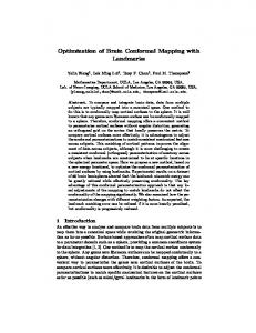
the “interior mapping problem” (1.2.1)–(1.2.2) by means of the transformation z → 1/z. b and maps the domain ΩE onto the This simple inversion transforms Γ into a Jordan curve Γ b i.e. onto the domain Ω b := Int(Γ). b Therefore, if fb is the conformal mapping interior of Γ, b → D1 , fb : Ω

(1.2.11)

normalized by the conditions fb(0) = 0

0 and fb (0) > 0,

(1.2.12)

then (see Figure 1.1) fE (z) = 1/fb(1/z).

(1.2.13)

Corresponding to the Definition 1.2.1 of the conformal radius, we have the following definition of an important geometric functional associated with the conformal mapping (1.2.9)– (1.2.10): Definition 1.2.2 (Capacity of a Jordan curve) Let Γ be a closed Jordan curve and assume that 0 ∈ Int(Γ). Also let ΩE := Ext(Γ) and let fE be the conformal mapping (1.2.9)–(1.2.10). Then the real constant 1 cap(Γ) := 0 , (1.2.14) fE (∞) is called the capacity of the curve Γ. From (1.2.13) we have that 0

cap(Γ) = fb (0) =

1 b R0 (Ω)

.

(1.2.15)

b := Int(Γ) b with respect Thus, cap(Γ) is the reciprocal of the conformal radius of the domain Ω to the origin. Remark 1.2.1 Definition 1.2.2 is restricted to bounded Jordan curves. This is sufficient for our purposes. For the definition in the more general case where Γ is a compact set the interested reader should consult, for example, [142, §5.1–5.3] and [147, pp. 24–25] where also the properties of cap(Γ) are discussed in detail. Here, we only note the elementary property that cap(Γ) remains invariant under translation and rotation of Γ.

6


Ωe Γ 0

fE

Ω

0

1

w − plane

z − plane

1/z

1/w

b Γ 0

fb

0

1

b Ω

Figure 1.1 We end this section by giving the definition of yet another geometric functional, the so-called “exponential radius” of a Jordan arc joining two parallel straight lines. This was introduced by Gaier and Hayman [58, §2], in connection with the theory of the domain decomposition method that we shall study in Section 3.9. Let γ be a Jordan arc that joins the lines Im z = 0 and Im z = 1 and lies entirely within the strip {z : 0 < Im z < 1}, except for its end points. Also, let γ ∗ be the arc obtained by translating γ along the real axis until it lies in Re z ≥ 0, with at least one point on Re z = 0. ∗ Next, let Γ∗ be the image of γ ∗ under the transformation z → eπz , and let Γ denote the ∗ reflection of Γ∗ in the real axis. Finally, let Γ denote the symmetric Jordan curve Γ := Γ∗ ∪Γ , and observe that Γ surrounds the unit circle and meets the circle in at least one point; see Figure 1.2.


7

i

γ

g

S−

∗

γ

G−

0

w − plane

b

i

0

z − plane

a

Z = eπz

W = eπw

Γ∗ Ω D1 0

f

1

1

0 ∗

Γ

Figure 1.2

Definition 1.2.3 (Exponential radius of an arc) With reference to Figure 1.2 and the no∗ tations introduced above, let Ω denote the Jordan domain Ω := Int(Γ∗ ∪ Γ ). Then, the exponential radius re (γ) of the arc γ is defined to be the conformal radius R0 (Ω) of the domain Ω with respect to the origin 0. In other words, re (γ) =

1 , f (0) 0

(1.2.16)

where f is the conformal mapping ∗

f : Ω := Int(Γ∗ ∪ Γ ) → D1 ,

(1.2.17)

normalized by the conditions f (0) = 0

0

and f (0) > 0.

(1.2.18)

8


Remark 1.2.2 If, instead of the lines Im z = 0 and Im z = 1, the arc γ joins the lines Re z = 0 and Re z = 1, then the exponential radius re (γ) is again given by Definition 1.2.3, but now: (i) γ ∗ is the arc obtained by translating γ along the imaginary axis until it lies in Im z ≤ 0, with at least one point on Im z = 0, (ii) Γ∗ is the image of γ ∗ under the ∗ transformation z → eiπz , and (as before) (iii) Γ is the reflection of Γ∗ in the real axis. Remark 1.2.3 (See also Exercise 1.14.) It is important to note that 1 ≤ re (γ) ≤ 4,

(1.2.19)

where the number 4 in the right-hand side of the inequality cannot be replaced by a smaller number. As for the proof of (1.2.19), the left inequality follows immediately from the increasing property (1.2.8), while the right is a consequence of the so-called Koebe 14 -theorem. This theorem states that if ϕ is any function which is analytic and univalent in D1 and such that ϕ(0) = 0 and ϕ0 (0) = 1, then the range ϕ(D1 ) of ϕ contains the disc with center the origin and radius 41 . Furthermore, the radius of this disc cannot be replaced by a number larger than 14 ; see e.g. [37, Theorem 2.3] and [62, p. 49, Theorem 2]. Remark 1.2.4 The exponential radius of an arc γ admits an alternative interpretation as follows; see [134, p. 112]: With reference to Figure 1.2, let G− denote the strip that lies to the left of the arc γ and let a and b denote, respectively, the points where γ intersects the lines Im z = 0 and Im z = 1. Also, let S− denote the strip S− := {w : Re w < 0, 0 < Im w < 1}, and let g be the conformal mapping g : S− → G− normalized by the conditions g(0) = a,

g(i) = b and

lim g(w) = ∞.

w→∞ w∈S−

Finally, let σ := min{Re z : z ∈ γ}. Then, the exponential radius r := re (γ) can also be defined by means of the relation lim

Re{w}→−∞ w∈S−

{g(w) − w} =

1 log r + σ. π

(1.2.20)

This can be deduced from the following observations: • The transformation w → eπw takes S− onto the upper half of the unit disc D1 . ∗

• The function F := f [−1] (which maps conformally D1 onto Ω := Int(Γ∗ ∪ Γ )) is related to the mapping function g by means of ½ µ ¶ ¾ 1 F (W ) = exp πg log W − πσ ; π see Figure 1.2.

1.3. THE MAPPING OF DOUBLY-CONNECTED DOMAINS •

µ log r = log F 0 (0) = lim log W →0

1.3

F (W ) W

9

¶ =π

lim

Re{w}→−∞ w∈S−

{g(w) − w} − πσ.

The mapping of doubly-connected domains

We start this section by observing that a conformal mapping is continuous and, as a result, preserves the order of connectivity. Thus, in particular, any conformal mapping of a doublyconnected domain is again a doubly-connected domain. It is, therefore, necessary for our work here to introduce a standard doubly-connected canonical domain to take the place of the unit disc, the canonical domain that we used in the simply-connected case. An obvious candidate for this is, of course, a circular annulus. In the doubly-connected case, however, we encounter a difficulty which was not present in the simply-connected case. This can be explained as follows: By the Riemann mapping theorem (Theorem 1.2.1), any simply-connected domain (whose boundary consists of more than one point) can be mapped onto the unit disc. From this it follows that all simply-connected domains are conformally equivalent, i.e. they can be mapped conformally onto each other. However, the same is not true in the case of doubly-connected domains. As the following theorem shows, not all doubly-connected domains are conformally equivalent. Theorem 1.3.1 Any doubly-connected domain, such that each of its boundary components consists of more than one point, can be mapped conformally onto a circular annulus of the form A(a, b) := {w : a < |w| < b}, (1.3.1) but only for a certain unique value of the ratio b/a of the two radii of the annulus. Definition 1.3.1 (Conformal modulus) Let A(a, b) be a circular annulus of the form (1.3.1). Then, the unique value of the ratio b/a for which a doubly-connected domain Ω is conformally equivalent to A(a, b) is called the conformal modulus of Ω and is denoted by M (Ω). In other words the conformal modulus M (Ω) of a doubly-connected domain Ω determines completely its conformal equivalence class, in the sense that two doubly-connected domains can be mapped onto each other if and only if they have the same modulus. The following theorem extends the result of Theorem 1.2.2 to the doubly-connected case: Theorem 1.3.2 Let Γ1 and Γ2 be two closed Jordan curves, such that Γ2 is in the interior of Γ1 , denote by Ω the doubly-connected domain Ω := Int(Γ1 ) ∩ Ext(Γ2 ),

(1.3.2)

10


and let ζ and b (0 < b < ∞) be respectively a fixed point on Γ1 and a prescribed number. Then, for a certain unique value a (0 < a < b) there exists a unique conformal mapping f : Ω → A(a, b)

(1.3.3)

(of Ω onto the circular annulus (1.3.1)), normalized by the condition f (ζ) = b.

(1.3.4)

Moreover, f can be extended one-one continuously to the closure Ω := Ω ∪ ∂Ω of Ω. In particular, the theorem says that if M := M (Ω) is the conformal modulus of the domain Ω, then the condition (1.3.4) determines uniquely the radius a = b/M , of the inner boundary of A(a, b), and ensures that the boundary curves Γ1 and Γ2 are mapped respectively onto the two boundary circles |w| = b and |w| = a. We consider next a relation that exists between the conformal mappings: (i) of a simplyconnected domain of a special type onto a rectangle, and (ii) of an associated symmetric doubly-connected domain onto a circular annulus. This relation is needed for the development of the theory of the domain decomposition method that we shall study in Chapter 3. Let Ω be a simply-connected domain of the form illustrated in Figure 1.3 (a). That is, Ω is bounded by a segment of the positive real axis, a straight line inclined at an angle π/n, (n ∈ N, n ≥ 1) to the real axis, and two Jordan arcs γ1 and γ2 that meet the two straight lines at the points z1 , z2 , z3 and z4 . Also, let the arcs γ1 := (z1 , z2 ) and γ2 := (z3 , z4 ) be given in polar co-ordinates by γj := {z : z = ρj (θ)eiθ , 0 ≤ θ ≤ π/n}, j = 1, 2,

(1.3.5)

b be the 2n-fold symmetric doubly-connected where 0 < ρ2 (θ) < ρ1 (θ), θ ∈ [0, π/n], and let Ω domain which is obtained by first reflecting Ω about the line θ = π/n and, if n > 1, continuing to reflect each new reflected part about the lines θ = jπ/n, j = 2, . . . , 2n − 1, respectively. That is, b := Int(Γ1 ) ∩ Ext(Γ2 ), Ω (1.3.6) where Γj := {z : z = ρbj (θ)eiθ , 0 ≤ θ ≤ 2π}, j = 1, 2, with ρbj (θ) = ρj (θ), θ ∈ [0, π/n], ρbj (kπ/n + θ) = ρbj (kπ/n − θ), θ ∈ [0, π/n], k = 1(1)2n − 1.

(1.3.7) ) (1.3.8)

b is the conformal modulus of the domain Ω, b there Then, for q = 1/M , where M := M (Ω) b → A(q, 1) of Ω b onto the circular annulus exists a conformal mapping f : Ω A(q, 1) := {ζ : q < |ζ| < 1},

(1.3.9)

which takes Γ1 and Γ2 onto the circles |ζ| = 1 and |ζ| = q and the points z1 , z2 , z3 and z4 onto the points ζ1 = 1, ζ2 = eiπ/n , ζ3 = qeiπ/n and ζ4 = q; see Theorem 1.3.2.

1.3. THE MAPPING OF DOUBLY-CONNECTED DOMAINS

11

z2

z3 z4

z3 0

Ω

γ2

π/n z4

γ2

γ1

eiαπ

1), then the first derivative of the mapping function f becomes unbounded at z = zc . Furthermore, because of the logarithmic terms in (1.4.1), a branch point singularity might occur even when 1/α is an integer. With reference to the last observation, when α = 1/N , with N ∈ N, then the “lowest” logarithmic term that might be present in (1.4.1) is (z − zc )2N log(z − zc ). differentiability properties of a conformal mapping at some boundary point depend only on the local structure of the boundary and not on the connectivity of the domain. ‡ This can be deduced from the Schwarz-Christoffel formula, which will be studied in § 1.5.2.

14


Thus, the question of when the corresponding coefficient BN,1,1 is nonzero is of some considerable interest. It is worth noting that Gaier addressed this question in [56], and derived a sufficient condition (involving the curvatures of the two arcs that form the arms of zc ) for BN,1,1 6= 0 (cf. [56, Theorem 3]).

1.4.2

Pole-type singularities

These are singularities that the mapping function (or, more precisely, its analytic extension) may have in the complement of the closure of the domain under consideration. We consider first the case of the conformal mapping (1.2.1)–(1.2.2). That is, we let Ω be a Jordan domain, denote by f the conformal mapping f : Ω → D1 normalized by the conditions f (z0 ) = 0 and f 0 (z0 ) > 0 (where z0 is some point in Ω), and consider the problem of determining the dominant singularities of the analytic extension of f in C \ Ω. (Here, by “dominant” singularities we mean the singularities that are closest to the boundary ∂Ω.) It turns out that if ∂Ω consists of straight lines and circular arcs, then these singularities of f can be determined easily by making use of the celebrated Schwarz reflection (or symmetry) principle which is stated below. b Theorem 1.4.1 (The Schwarz reflection principle; see e.g. [116, p. 184]) Let Ω and Ω b contain respectively be two simply-connected domains and let their boundaries ∂Ω and ∂ Ω circular arcs γ and γ b (which may degenerate into straight line segments). If the function F b in such a way that γ maps conformally Ω onto Ω b corresponds to γ, then F can be continued ∗ analytically into the domain Ω obtained from Ω by inversion with respect to the circle (straight line) C of which γ forms a part. If z ∈ Ω and z ∗ ∈ Ω∗ are symmetric (inverse) points with respect to C, then F (z) and F (z ∗ ) are symmetric points with respect to the circle (straight b of which γ line) C b forms a part. Consider now the conformal mapping f : Ω → D1 , assume that part of ∂Ω consists of a circular arc or straight line segment γ, and observe that f maps γ onto an arc γ b of the unit circle |w| = 1. Also, recall the normalization condition f (z0 ) = 0, and let z0∗ ∈ C \ Ω be the symmetric point of z0 with respect to the circle (straight line) of which γ forms part. Then, since the symmetric point of 0 with respect to the unit circle is the point at ∞, it follows from Theorem 1.4.1 that the analytic extension of f has a simple pole at z0∗ . In other words, if ∂Ω consists of straight line segments and circular arcs, then the mapping function (1.2.1)–(1.2.2) has simple pole singularities at the mirror images (in C \ Ω) of the “normalization” point z0 with respect to the straight lines, and at the symmetric points (in C \ Ω) of z0 with respect to the circles of which the circular arcs form part. If ∂Ω is more general than a curve consisting of straight lines and circular arcs, then the problem of determining the location and nature of singularities of the mapping function f in C \ Ω is much more complicated, and involves using the generalized symmetry principle for analytic arcs; see e.g. [148, p. 102]. The basic details are as follows:

1.4. SINGULARITIES OF THE MAPPING FUNCTION

15

Let γ be an analytic arc of ∂Ω with analytic parametric equation z = τ (s),

s1 ≤ s ≤ s2 ,

(1.4.4)

and (for simplicity) assume that z0 = 0 in the normalizing condition (1.2.2). Then, the general procedure for determining the singularities of the analytic extension of f across γ involves examining the zeros of the function τ (ζ) (of the complex variable ζ = s + it) and of its derivative τ 0 (ζ). This comes about from the generalized symmetry principle, which states that the analytic extension of f across γ is given by {f (I(z))}−1 ,

(1.4.5)

I(z) := τ {τ [−1] (z)}.

(1.4.6)

where Here, I(z) defines the symmetric point of z with respect to γ, and is independent of the choice of the parametrization of γ. From this it follows, for example, that if ζ ∗ is a simple zero of τ (ζ) and certain other conditions (concerning the proximity of ζ ∗ to γ) hold, then the mapping function f has a simple pole at the symmetric point of the origin with respect to γ, i.e. at the point z ∗ = I(0) = τ (ζ ∗ ). (1.4.7) Although simple poles are the most frequently occurring singularities, other types of singularities may also occur. For example, depending on the multiplicity of the root ζ ∗ and its position relative to γ, f may have a double pole of the form 1 , (z − z ∗ )2

(1.4.8)

or a branch-point singularity of the form f (z) ∼ (z − z ∗ )−m/n

m, n ∈ N,

as z → z ∗ ,

(1.4.9)

at the symmetric point (1.4.7). We consider next the exterior mapping problem (1.2.9)–(1.2.10) and note the following in connection with our computational work in Chapter 2: (i) For reasons that will become apparent in § 2.4.3 and § 2.6.1, we are now interested in the singular behavior of the intermediate “interior” mapping function fb defined by (1.2.11)–(1.2.12). (ii) The inversion zb = 1/z (that carries the boundary Jordan curve Γ onto the Jordan curve c b and maps the exterior domain ΩE := Ext(Γ) onto the interior domain Ω b := Int(Γ)) Γ makes it less likely for the mapping function fb to have simple pole singularities or b singularities of the forms (1.4.8)–(1.4.9) in C \ Ω.

16


Intuitively, the observation in (ii) above can be explained as follows: As before, let γ be an analytic arc of Γ := ∂ΩE with analytic parametric equation (1.4.4). Then, under the inversion zb → 1/z, γ is transformed into an analytic arc γ b with parametric equation zb = τb(s),

s1 ≤ s ≤ s2 ,

where τb(s) = 1/τ (s).

(1.4.10)

Next, recall that simple pole singularities and singularities of the forms (1.4.8)–(1.4.9) occur at points z ∗ = τb(ζ ∗ ) where ζ ∗ is a root of the equation τb(ζ) = 0.

(1.4.11)

But, (1.4.11) can only have a root at a point where τ becomes unbounded. Thus, if (as is frequently the case) τ is an entire function, then fb cannot have simple pole or singularities of the forms (1.4.8)–(1.4.9). In particular, the following can be deduced directly from the Schwarz reflection principle (i.e. Theorem 1.4.1), by recalling that such singularities occur at symmetric points of the origin of the zb-plane: (i) If the boundary curve Γ is a polygon, then fb has no pole-type singularities. To see this, recall that the inversion zb = 1/z transforms any straight line in the z-plane onto a generalized circle (i.e. a straight line or a circle) passing through the origin of the zb-plane; see Exercise 1.6. (ii) If Γ consists of straight line segments and circular arcs, then the only possible pole-type singularities of fb are due to the circular arcs. More precisely, a singularity occurs if the center of a circular arc γ is in Int(Γ) and does not coincide with the origin of the b z-plane. If zc is such a center, then fb has a simple pole at the point zbc = 1/zc ∈ Ext(Γ). ∗ To see this observe that the points zc and zc = ∞ are symmetric with respect to γ. Therefore, zbc = 1/zc and the origin of the zb-plane are symmetric with respect to the image of γ under the inversion zb = 1/z. All the above, about the singularities in C \ Ω of the interior and exterior mapping functions for simply-connected domains, are studied in detail in [137] and [138, §5]. In the doubly-connected case, the situation regarding the singular behavior (in C \ Ω) of the mapping function (1.3.3)–(1.3.4) is more complicated and less satisfactory than in the case of simply-connected domains. As far as we are aware, the only relevant information is given in [135], where it is shown that in many cases both the mapping function f and the auxiliary function f 0 (z) 1 H(z) := − , (1.4.12) f (z) z

1.5. NUMERICAL CONFORMAL MAPPING

17

(which, as will be seen, plays a very central role in the numerical methods of Section 2.5) have singularities in the so-called “common symmetric points” with respect to the two boundary components of the doubly-connected domain. As in Section 1.3, let Ω := Int(Γ1 ) ∩ Ext(Γ2 ) and let γ1 and γ2 be analytic arcs of the outer and inner boundary components Γ1 and Γ2 of Ω. Also, let (z, Ij (z)), j = 1, 2, denote pairs of symmetric points with respect to the arcs γj , j = 1, 2, respectively. Then, two points z1 ∈ Ext(Γ1 )

and z2 ∈ Int(Γ2 ),

(1.4.13)

are said to be common symmetric points with respect to γ1 and γ2 if z1 = Ij (z2 ) and z2 = Ij (z1 ), j = 1, 2,

(1.4.14)

i.e. if z1 , z2 are symmetric with respect to both γ1 and γ2 or, equivalently, if they are both fixed points of the two composite functions S1 := I1 ◦ I2

and S2 := I2 ◦ I1 .

(1.4.15)

Although there are geometries for which no common symmetric points exist, there are cases for which the points z1 and z2 can be determined easily from the functions (1.4.16); see e.g. Exercises 1.20 and 1.21. In such cases, an analysis based essentially on the repeated application of the Schwarz reflection principle shows that, under certain conditions, the points z1 and z2 are singular points of both the mapping function f and the function H defined by (1.4.12). In particular, it is shown in [135] that the singular behavior of the function H, at z1 , z2 , can be reflected approximately by that of simple poles at z1 , z2 , i.e. by that of the functions 1 , j = 1, 2. (1.4.16) z − zj

1.5

Numerical conformal mapping

From the computational point of view, the problems of approximating the conformal mapping Ω → D1 (of a simply-connected domain Ω onto the unit disc D1 ) and the inverse mapping D1 → Ω are by far the most extensively studied numerical conformal mapping problems. As a result, there are several efficient numerical methods, and also a number of software packages in the public domain, for computing approximations to both Ω → D1 and D1 → Ω. There are also several numerical methods for approximating the conformal mapping Ω → A(a, b), of a doubly connected domain Ω onto a conformally equivalent annulus of the form (1.3.1), and the inverse mapping A(a, b) → Ω. As far as we are aware, however, there are no as yet well-tested computer packages for the mapping of doubly-connected domains. (See, however, Remark 1.5.14 in Section 1.5.2 below.)

18


In Chapter 2 we shall study in detail both the theoretical and the computational aspects of a class of orthonormalization methods for the conformal mapping of simply and doublyconnected domains, and shall also consider the extension of these methods to the mapping of n-connected domains with n > 2. First, however, we give brief outlines of two other important numerical methods: (i) the so-called “integral equation method of Symm”, and (ii) a SchwarzChritoffel transformation method for the mapping of simply-connected polygonal domains. These two methods are of special interest, because they can both deal with regions involving corners, and also because each of the methods can be implemented by means of available (and highly effective) computer software.

1.5.1

The integral equation method of Symm

The method is for approximating the conformal mappings of interior and exterior simplyconnected domains as well as doubly-connected domains, and is based on three closely related formulations that were originally proposed by G.T. Symm in [157], [158] and [159] respectively. In each case, the method involves solving a weakly singular Fredholm integral equation of the first kind for an unknown density function ν; see Remark 1.5.7. In what follows we give an outline of the formulation that corresponds to the interior mapping problem. Let Ω be a simply-connected domain bounded by a closed Jordan curve Γ, assume that 0 ∈ Ω, and let f denote the conformal mapping f : Ω → D1 , normalized by the conditions f (0) = 0 and f 0 (0) > 0. Also, let the parametric equation of the boundary curve Γ = ∂Ω be z = τ (s),

0 ≤ s ≤ L,

(1.5.1)

where s is some appropriate parameter (not necessarily arc length), and assume that (1.5.1) defines a positive orientation of Γ with respect to Ω. Finally, let θ be the boundary correspondence function associated with the conformal mapping f . This is defined by f (τ (s)) = exp(iθ(s)), i.e. θ(s) = arg(f (τ (s)),

(1.5.2)

where arg(·) is a continuous argument as described, for example, in [74, §4.6] and [91, §11.7]. One way for deriving Symm’s integral equation formulation for the conformal mapping Ω → D1 is by observing that the function log{f (z)/z} is analytic in Ω, writing the mapping function f as f (z) = z exp(u(z) + iv(z)), z ∈ Ω, (1.5.3) where u and v are conjugate harmonic functions in Ω, and expressing the function u as a single layer potential Z L u(z) = ν(s) log |z − τ (s)| ds, z ∈ Ω, (1.5.4) 0

for an unknown density function ν. Then, by imposing the boundary condition u(z) = − log |z|,

z ∈ Γ,

(1.5.5)

1.5. NUMERICAL CONFORMAL MAPPING we are led to the integral equation Z L ν(s) log |τ (σ) − τ (s)| ds = − log |τ (σ)|,

19

0 ≤ σ ≤ L,

(1.5.6)

0

for the density function ν; see Remark 1.5.7. Regarding the solvability of (1.5.6), it is shown in [46] that this integral equation has a unique solution provided that cap(Γ) 6= 1, (1.5.7) where cap(Γ) is the capacity of the boundary curve Γ; see Definition 1.2.2. (This means that (1.5.6) always has a unique solution, subject only to a possible re-scaling of Γ = ∂Ω.) It is also shown in [46] that if the condition (1.5.7) holds, then the unique solution of (1.5.6) is related to the boundary correspondence function θ (see (1.5.2)) by means of ν(s) = −

1 dθ . 2π ds

(1.5.8)

Once the solution ν of (1.5.6) is found, then (because of (1.5.3) and (1.5.4)) the mapping function f is given by µZ L ¶ f (z) = z · exp ν(s) log(z − τ (s)) ds , z ∈ Ω. (1.5.9) 0

We make the following remarks about the formulation (1.5.6), (1.5.9) and its extensions, and about the numerical methods and software that are available for the solution of the integral equation (1.5.6). Remark 1.5.1 As was previously remarked, Symm also considered the exterior and doublyconnected mappings and gave integral equation formulations for these two problems in [158] and [159] respectively. There are, however, two alternative formulations due to Gaier ([46] and [49]) that present certain important advantages over those of Symm, in cases where the boundary of the domain under consideration involves corners; see e.g. [121, pp. 26-27]. In addition, in [46] and [49], Gaier gave a rigorous treatment of the theory of each of the three formulations (i.e. for the interior, exterior and doubly-connected mappings) and, in particular, resolved completely the questions of existence and uniqueness of the solutions of the associated integral equations. Remark 1.5.2 Assume that part of the boundary curve Γ consists of two analytic arcs that meet at a point zc = τ (sc ) and form there a corner of interior angle απ, where 0 < α < 2. Then it can be shown (by using the Lehman expansions (1.4.1)–(1.4.3) and considering the asymptotic behavior of dθ/ds near s = sc ) that the leading term of the asymptotic expansion of the density function ν in the neighborhood of s = sc is always of the form a(s − sc )−1+1/α ,

(1.5.10)

20


where a 6= 0; see [84, §2], [85, §3], [138, §4.2] and [121, §3] and also Exercise 1.24. This means, in particular, that: (i) if 1 < α < 2, i.e. if the corner is re-entrant, then ν becomes unbounded at s = sc , and (ii) if 1/(N + 1) < α < 1/N , with N ∈ N, then ν (N ) becomes unbounded at s = sc . In other words, in the case of a piecewise analytic boundary, the density function ν might have serious boundary singularities at the corner points of Γ. Remark 1.5.3 Regarding numerical methods, the original method proposed by Symm in [157] is based essentially on: (i) approximating the unknown density function ν, in the integral equation (1.5.6), by a step function νe, (ii) determining the approximation νe by collocation (see Remark 1.5.7) at an appropriate number of boundary points, and (iii) computing the approximations to the mapping function f from (1.5.9), with ν replaced by νe. A similar, but more refined, collocation method is proposed in [71]. This involves using C 0 piecewise defined quadratic polynomials (instead of step functions) for the approximation of ν. It should be observed, however, that the methods of [157] and [71] do not provide any special treatment for the singularities that ν might have at corner points on the boundary curve Γ. For this reason, the methods are not recommended for the mapping of regions with corners. Remark 1.5.4 In [84] the difficulties associated with corner singularities are treated by using a numerical method based on: (i) approximating the source density ν by splines of various degrees, (ii) modifying the spline approximation by introducing, in the neighborhood of each corner, singular functions that reflect the main singular behavior of ν, and (iii) blending the singular functions with the splines that approximate ν on the remainder of Γ, so that the global piecewise defined approximating function has continuity of appropriate order at the transition points between the two types of approximation. The same approach is used in [85], in conjunction with the exterior and doubly-connected formulations of Gaier [46], [49], for the approximation of the exterior and doubly-connected mappings; see also [121, §3] and [138, §4.2]. Remark 1.5.5 Other publications that deal with various theoretical and numerical aspects of the integral equation method of Symm are [23], [79], [80], [81] [83], [88], [104], [174], [176] and [177]. Remark 1.5.6 Regarding numerical software, there is an excellent and highly automated conformal mapping package based on the integral equation formulation (1.5.6), (1.5.9) of Symm. This is the FORTRAN package CONFPACK of Hough [82]. The package is based on a collocation method, and involves the judicious use of Jacobi polynomials for: (i) approximating the density function ν, (ii) reflecting the corner singularities (1.5.10) of ν, and (iii) performing the necessary quadratures; see also [80] and [81]. In addition to the mapping Ω → D1 , CONFPACK can also deal with the problems of approximating the inverse mapping D1 → Ω, as well as the exterior mapping C \ Ω → {w : |w| > 1} and its inverse. CONFPACK is available at Netlib and (at the time of writing) can also be obtained from the author’s


21

webpage§ . A more recent double precision version of the package is also available from the author’s webpage.

Remark 1.5.7 Equation (1.5.6) is a linear “Fredholm integral equation of the first kind”. In general, such equations are of the form Z

b

K(σ, s)ν(s)ds = µ(σ),

(1.5.11)

a

where a and b are fixed numbers, the “kernel” K(σ, s) and the “driving term” µ(σ) are known for a ≤ σ, s ≤ b and a ≤ σ ≤ b, respectively, and ν is the sought unknown function. Thus, Equation (1.5.6) has a logarithmic (and hence “weakly singular”) kernel K(σ, s) = log |τ (σ) − τ (s)|. The “method of collocation” for solving (1.5.11) involves the following: (i) Approximating the unknown function ν by νn (σ) :=

n X

c` κ` (σ),

(1.5.12)

`=1

where {κ` }n`=1 is a suitably chosen set of linearly independent functions. (ii) Determining the coefficients c` , in (1.5.12), by requiring that the residual function Z rn (σ) :=

b

K(σ, s)νn (s)ds − µ(σ),

a

is zero at n distinct points σk , k = 1, 2, . . . , n, in [a, b]. That is, the approximation (1.5.12) is determined by solving the n × n linear system Ac = µ, where A = {ak,` } is the n × n matrix with elements Z ak,` =

b

a

K(σk , s)κ` (s)ds,

and c, µ are respectively the n-dimensional vectors c = [c1 , c2 , . . . , cn ]T

§

and µ = [µ(σ1 ), µ(σ2 ) . . . , µ(σn )]T .

http://www.mis.coventry.ac.uk/∼dhough/

22

1.5.2


Schwarz-Christoffel mappings

By Schwarz-Christoffel mappings we mean the family of methods that are based on the use of the well-known Schwarz-Christoffel formula, the underlying theory of which is treated extensively in the complex variables literature; see e.g. [1, §5.6], [74, §5.12], [116, §6], [145, §7.5 and Appendix A]. Although the formula is usually given in connection with the conformal mapping of the upper half-plane onto a polygonal domain Ω, here (for the sake of uniformity) we prefer to start by considering the equivalent formulation which is for the mapping f : D1 → Ω, of the unit disc D1 onto Ω. We state the corresponding formula in the form of a theorem. Theorem 1.5.1 (Schwarz-Christoffel formula) Let Γ be a polygon with vertices (in counterclockwise order) at the points w1 , w2 , . . . , wn , let α1 π, α2 π, . . . , αn π be respectively the (interior) angles of the vertices w1 , w2 , . . . , wn , and let Ω denote the polygonal domain Ω := Int(Γ). If f : D1 → Ω is any conformal mapping of the unit disc D1 := {z : |z| < 1} onto Ω, then ¶ Z zY n µ ζ αk −1 1− f (z) = A dζ + B, (1.5.13) zk 0 k=1

where zk , k = 1, 2, . . . , n, are the pre-images of the vertices wk , k = 1, 2, . . . , n, i.e. f (zk ) = wk , k = 1, 2, . . . , n,

(1.5.14)

and A, B are integration constants which are determined by the position and size of the polygon. Formula (1.5.13) applies to polygons that have slits (i.e. vertices with angles 2π) and infinite polygons (i.e. with vertices at infinity), and it can also be adapted easily to the exterior conformal mapping {z : |z| > 1} → Ext(Γ); see e.g. [1, p. 352] and [116, p. 193]. From the constructive point of view, however, there is a major difficulty. This has to do with the fact that formula (1.5.13) involves the “pre-vertices” zk , k = 1, 2, . . . , n, on the unit circle (i.e. the pre-images of the vertices wk of Ω) which are not known a priory. The problem of determining these pre-vertices is the so-called Schwarz-Christoffel “parameter problem”. Solving this problem is a major numerical task of any Schwarz-Christoffel mapping procedure. In addition, numerical quadrature is needed for approximating the integrals involved in the parameter problem, and also for determining the transformation itself from (1.5.13). Finally, considerable computational effort is needed for inverting the conformal mapping, i.e. for computing the mapping Ω → D1 . For full details of the above we refer the reader to the recent monograph on SchwarzChristoffel mappings by Driscoll and Trefethen [35], which contains a thorough study of the computational aspects of the subject covering all major developments up to 2002. Here, we shall only make the following brief remarks in order: (i) to outline the main computational steps involved in the process, and (ii) to indicate the available numerical software.


23

Remark 1.5.8 Let zk = eiθk , k = 1, 2, . . . , n. Then, for the solution of the parameter problem, the three degrees of freedom of the mapping may be used to fix the positions of three of the pre-vertices on the unit circle, i.e. of three of the arguments θk , k = 1, 2, . . . , n.

(1.5.15)

The other n − 3 unknown real parameters in (1.5.13), i.e. the arguments of the remaining pre-vertices, can then be determined from the n − 3 real conditions ¯ ´αk −1 ¯¯ ¯R zj+1 Qn ³ ζ ¯ dζ ¯¯ k=1 1 − zk ¯ zj |wj+1 − wj | ¯ (1.5.16) ´αk −1 ¯¯ = |w − w | , j = 2, 3, . . . , n − 2. ¯R z2 Qn ³ 2 1 ζ ¯ ¯ 1 − dζ zk ¯ z1 k=1 ¯ (These ensure that the polygon obtained by the transformation (1.5.13) is similar to the given polygon Ω.) When solving the above system, it is essential that the pre-vertices zk are constrained to lie in the correct order on the unit circle ∂D1 . This can be achieved by requiring that 0 < θ1 < θ2 < · · · < θn ≤ 2π. (1.5.17)

Remark 1.5.9 The constrained nonlinear system (1.5.16)–(1.5.17), for solving the parameter problem, comes about as a consequence of the following fact: Let Ω be a bounded polygonal domain and assume (without loss of generality) that αn 6= 1 and αn 6= 2. Then, Ω is uniquely determined (up to scaling, rotation and translation) by its angles and the n − 3 side-lengths ratios on the right-hand side of (1.5.16); see [35, Theor. 3.1]. Only a slight modification of the system (1.5.16)–(1.5.17) is needed for dealing with polygons that have vertices at infinity; see [35, p. 25]. Remark 1.5.10 Any Schwarz-Christoffel procedure requires the computation, by means of numerical quadrature, of integrals of the form ¶ Z bY n µ ζ αk −1 1− dζ. (1.5.18) zk a k=1

In particular, the limits of integration a, b in the integrals that arise in (1.5.16) are, in general, pre-vertices. This means that, in general, the associated integrands involve singularities at both the two ends of integration. Therefore, care must be taken when choosing the numerical quadrature so that it can deal with such singularities. Remark 1.5.11 There are two computer packages available for the Schwarz-Christoffel mapping of a polygonal domain Ω onto the unit disc D1 . The first of these is the FORTRAN package SCPACK of Trefethen [165]. This is based on an algorithm proposed in [162], and is

24


regarded as the first fully automated program for conformal mapping. The main features of the underlying algorithm are as follows: (i) the integrations (1.5.18), needed for setting up the nonlinear system (1.5.16) for the parameters of the mapping and for determining the mapping function f from (1.5.13), are performed using a form of compound Gauss-Jacobi quadrature (see [35, §3.2]), (ii) by a simple change of variables, the parameter problem (1.5.16)–(1.5.17) is set up as an unconstrained nonlinear system in n − 1 real parameters, and is solved by using a packaged subroutine (see [35, §3.1]), and (iii) the inverse conformal mapping Ω → D1 is computed in two steps by means of a packaged ODE solver and Newton’s method (see [35, §3.3]). Like CONFPACK, SCPACK is available at Netlib. Remark 1.5.12 The second Schwarz-Christoffel package is the so-called MATLAB SC Toolbox of Driscoll [34]. In fact, the SC Toolbox may be regarded as a more capable successor of SCPACK. In addition, to the disc mapping Ω → D1 and its inverse, the package can also deal with the corresponding half-plane mappings as well as with exterior mappings. Moreover, the toolbox can deal with the following: (i) constructing the mapping of D1 onto a polygon using the cross ratios and Delaunay triangulation (CRDT) algorithm of Driscoll and Vavasis [36] (see also [35, §3.4] and our discussion in Section 3.7), (ii) constructing the mapping of an infinite strip {z : 0 < Imz < 1} onto a polygon (see [87] and [35, §4.2]), and (iii) constructing the mapping of a rectangle onto a polygon (see [35, §4.3]). (As will become apparent later, the techniques indicated in (i)-(iii) are of special interest to us in connection with some of the topics covered Chapter 3.) Further details about the SC Toolbox, together with information on how to obtain the package, can be found in [35, pp. 115–19]. Remark 1.5.13 If n is the number of vertices of the polygon, then the estimates of the CPU times in the algorithms used by SCPACK and the MATLAB SC Toolbox are, in both cases, O(n3 ) for solving the parameter problem, and (once the unknown parameters are determined) O(n) for computing the conformal mapping f at a specific point of Ω. In a recent paper [9], Banjai and Trefethen give a new implementation of the Schwarz-Christoffel method that reduces the above estimates to O(n log n) and O(log n) respectively, thus allowing for the mapping of polygons with tens of thousands of vertices. These cost reductions are achieved by: (i) considering the logarithm of the Schwarz-Christoffel integrand and using the fast multipole method, developed in [21], for computing the associated logarithmic sums, and (ii) using a simple iterative method given in [28] (rather than the more sophisticated nonlinear equation solvers used in SCPACK and the SC Toolbox) for the solution of the parameter problem. Several impressive examples involving the mapping of polygons with very large numbers of vertices (the largest of which is n = 196, 608!) can be found in [9, pp. 1052– 1064]. Remark 1.5.14 The Shwarz-Christoffel technique can be extended to the mapping of an annulus onto a polygonal doubly-connected domain, i.e. onto a doubly-connected domain bounded externally and internally by two polygonal curves. For further details of this we


25

refer the reader to [35, §4.9] and [31]. There is also a software package (the conformal mapping package DSPACK), due to Hu [89], for implementing such transformations. This package is available at Netlib. Finally, we note the recent papers of Crowdy [26] and DeLillo et al [32] on the extension of the Shwarz-Christoffel method to n-connected domains with n > 2. We conclude our discussion of Schwarz-Christoffel mappings with two remarks about: (a) the Schwarz-Christoffel formula for the mapping of the upper half-plane H+ := {z : Im z > 0} onto a polygonal domain Ω, and (b) the problem of determining an explicit expression for this formula in the important special case where Ω is a rectangular domain. Remark 1.5.15 The Schwarz-Christoffel formula, for the conformal mapping from the upper half-plane H+ onto a polygonal domain Ω, differs only slightly from the corresponding formula (1.5.13) that we chose to use for the mapping D1 → Ω. Thus, with the notations of Theorem 1.5.1, the mapping function f : H+ → Ω is given by Z f (z) = A

n z Y

0 k=1

(ζ − zk )αk −1 dζ + B,

(1.5.19)

where now the pre-vertices zk , k = 1, 2, . . . , n, lie on the real axis. If, as is frequently the case, the pre-vertex zn is chosen to be the point at infinity (i.e. if the condition f (∞) = wn is imposed), then the formula remains unaltered except that the factor corresponding to zn is deleted from the integrand in the right-hand side of (1.5.19). Note, however, that if this is done, then we are free to designate only two of the other pre-vertices. As for the derivation of (1.5.19), this involves considering a function f whose derivative is of the form n Y (ζ − zk )βk , βk = αk − 1, f 0 (z) = A k=1

noting that 0

arg f (z) = arg A +

n X

βk arg(z − zk ),

k=1

and showing that, as z traverses the real axis, f (z) generates a polygonal path whose tangent at the point f (zk ) makes a turn through an angle βk π; see e.g. [116, pp. 189–192] and [145, §7.5]. Regarding formula (1.5.13), for the conformal mapping D1 → Ω, this can be obtained from (1.5.19) by using an intermediate bilinear (Möbius) transformation that takes D1 onto H+ ; see e.g. [35, §4.1] and [116, pp. 192–193]. Remark 1.5.16 An inspection of (1.5.13) and (1.5.19) shows that for n > 4 it is not, in general, possible to express the integrals involved in the two Schwarz-Christoffel formulas in terms of elementary functions. Even in the case n = 4, there is no simple analytic way for determining the one degree of freedom in the pre-vertices. However, as it is shown below, in the important case where Ω is the interior of a rectangle, the symmetry of the domain allows

26


us to obtain an explicit solution of the problem of determining f : H+ → Ω by means of (1.5.19). Let 0 < k < 1, and consider the problem of determining a conformal mapping of the half-plane H+ onto a rectangle Ω, so that the four points z1 = −1, z2 = 1, z3 = 1/k and z4 = −1/k on the real axis are mapped, respectively, onto the four vertices of Ω. Then, from (1.5.19) we know that such a mapping is effected by the function Z z dζ −1 f (z) = (z, k), (1.5.20) 1 1 =: sn 0 (1 − ζ 2 ) 2 (1 − k 2 ζ 2 ) 2 where sn(·, k) denotes the Jacobian elliptic sine with modulus k. In order to determine the position and dimensions of the rectangle we first note that for real z, −1 < z < 1, f (z) is real and f (−z) = −f (z). This means that one of the sides of the rectangle coincides with part of the real axis and is situated symmetrically with respect to the origin. Further, Z 1 dx f (1) = (1.5.21) 1 1 =: K(k). 2 0 (1 − x ) 2 (1 − k 2 x2 ) 2 where K(k) denotes the complete elliptic integral of the first kind with modulus k. Hence, f (−1) = −K(k). Finally, it can be shown (see Exercise 1.26) that Z 1/k dx 0 (1.5.22) f (1/k) = 1 1 =: K(k) + iK(k ), 0 (1 − x2 ) 2 (1 − k 2 x2 ) 2 and hence that f (−1/k) = −K(k) + iK(k 0 ), where K(k 0 ) is the complete elliptic integral of the first kind with (complementary) modulus 1 k 0 = (1 − k 2 ) 2 . Therefore, the Schwarz-Christoffel transformation (1.5.20) maps conformally the upper half plane H+ onto the rectangle Ω := {(x, y) : −K(k) < x < K(k), 0 < y < K(k 0 )},

(1.5.23)

so that the four points z1 = −1, z2 = 1, z3 = 1/k and z4 = −1/k, on the real axis, go respectively to the four vertices w1 = −K(k), w2 = K(k), w3 = K(k) + iK(k 0 ) and w4 = −K(k) + iK(k 0 ) of Ω. Furthermore: (i) as is immediately clear f (0) = 0, and (ii) it can be shown that f (∞) = iK(k 0 ); see Exercise 1.26. The above Schwarz-Christoffel transformation, of the upper half-plane onto a rectangle, will play a very central role in our work in Chapter 3, where we shall also make extensive use of various properties of elliptic functions and integrals. For a detailed study of these properties the reader should consult the relevant literature; e.g. [18] and [116, pp. 280–296]. Here, we merely note the following: (i) The name Jacobian elliptic “sine” and the symbol sn are used to denote the function whose inverse is defined by (1.5.20), because of the analogies that sn presents with the trigonometric

1.6. NUMERICAL EXAMPLE

27

function sin. In fact, as it is easy to see, the function sin−1 z corresponds to the degenerate case that results by letting k → 0 in (1.5.20). This analogy is carried further by the definition p cn(w, k) = 1 − sn2 (w, k), cn(0, k) = 1, (1.5.24) for the “Jacobian elliptic cosine”, and the definition p dn(w, k) = 1 − k 2 sn2 (w, k),

dn(0, k) = 1,

(1.5.25)

for the Jacobian elliptic function dn. Also, the name “elliptic functions” is used because the integral (1.5.20) was first encountered in connection with the problem of finding the length of an arc of an ellipse. (ii) The fundamental property of the three elliptic functions is that each is “doubly-periodic”, i.e. that each has two different periods which are not integral multiples of the same number. For example, for sn(·, k) the periods are 4K(k) and 2iK(k 0 ), i.e. sn(w + 4K(k), k) = sn(w, k) and

sn(w + 2iK(k 0 ), k) = sn(w, k).

(1.5.26)

This can be shown by observing that z = sn(w, k) maps conformally the rectangle (1.5.23) onto the upper half-plane, and applying repeatedly the Schwarz reflection principle; see e.g. [116, pp. 282–283]. Similarly, for the functions cn(·, k) and dn(·, k) the pairs of periods are, respectively, 4K(k), 2K(k) + 2iK(k 0 ) and 2K(k), 4iK(k 0 ). (iii) The only zeros of sn(w, k) are simple zeros at the points w = 2mK(k) + 2niK(k 0 ),

m, n ∈ Z,

(1.5.27)

and the only finite singularities are simple poles at the points w = 2mK(k) + (2n + 1)iK(k 0 ),

1.6

m, n ∈ Z.

(1.5.28)

Numerical Example

The example that follows illustrates the remarkable accuracy that can be achieved by two of the conformal mapping packages that we discussed in Section 1.5.

28


z8

z1

Ω

z7

z2

z6

0 z3

z4

z5

Figure 1.4

Example 1.6.1 Let Ω be the L-shaped domain Ω := {(x, y) : −1 < x < 3, |y| < 1} ∪ {(x, y) : |x| < 1, −1 < y < 3},

(1.6.1)

illustrated in Figure 1.4, and let zj , j = 1, 2, . . . , 7, be the following points on ∂Ω: z1 = −1 + 3i, z2 = −1 + i, z3 = −1 − i, z4 = 1 − i, z5 = 3 − i, z6 = 3 + i, z7 = 1 + i, z8 = 1 + 3i.

(1.6.2)

Also, let f denote a conformal mapping f : Ω → D1 , of Ω onto the unit disc, and let ζj = f (zj ),

j = 1, 2, . . . , 8,

(1.6.3)

be respectively the images of the points zj , j = 1, 2, . . . , 8, on ∂D1 . Finally, let c1 , c2 and c3 denote the cross-ratios c1 := {ζ1 , ζ3 , ζ5 , ζ6 }, c2 := {ζ8 , ζ4 , ζ6 , ζ7 } and c3 := {ζ8 , ζ1 , ζ3 , ζ6 },

(1.6.4)

and recall that: (i) the cross-ratio c := {α1 , α2 , α3 , α4 }, of four distinct points αj , j = 1, 2, 3, 4, in the complex plane, is given by c := {α1 , α2 , α3 , α4 } =

α1 − α3 α2 − α4 · , α1 − α4 α2 − α3

and (ii) cross-ratios remain invariant under bilinear transformations; see Exercise 1.8.

(1.6.5)

1.6. NUMERICAL EXAMPLE

29

With reference to the points (1.6.3), it was shown by Gaier [45, p. 189] (using symmetry arguments) that there exists a bilinear transformation that maps D1 onto the upper half-plane H+ := {t : Im t > 0}, so that √ ζ1 → 1 − 3, ζ2 → 0, ζ3 → 1, ζ4 → 2, √ (1.6.6) ζ5 → 1 + 3, ζ6 → 3, ζ7 → ∞, ζ8 → −1. From this it follows that if the points αj , j = 1, 2, 3, 4, come from the set (1.6.3), then the cross-ratio (1.6.5) can be calculated exactly. In particular, the exact values of the cross-ratios (1.6.4) are, respectively, c1 = 4(2 −

√ 3),

c2 = 4,

1 1 and c3 = √ + , 3 2

(1.6.7)

i.e. to 17 decimal places, c1 = 1.071 796 769 724 490 83,

c2 = 4,

and c3 = 1.077 350 269 189 625 77 ;

(1.6.8)

see also Example 3.6.1 in Section 3.6 below. Since f is not known exactly, in what follows we shall use (1.6.8) as comparison values for checking the accuracy of the computed approximations to f . In Table 1.1 we list the values of the approximations to c1 , c2 and c3 that we computed using, respectively, the double precision version of CONFPACK (see Remark 1.5.6), and the Schwarz-Christoffel package SCPACK (see Remark 1.5.11). We make the following remarks in connection with the use of the two packages and the quality of the resulting approximations: (i) The computations were performed using double precision FORTRAN on a UNIX environment. (ii) The CONFPACK results were obtained by applying the package with 940 collocation points. The CONFPACK error estimate for the approximation to f is 5.1 × 10−13 . (iii) For the application of the SCPACK, apart from the physical corners z1 , z3 , z5 , z6 , z7 of the L-shape, the point z4 (whose image is involved in the cross-ratio c2 ) was also defined as a “corner”. The SCPACK error estimate is 3.8 × 10−14 . (iv) The results of Table 1.1 indicate that both the CONFPACK and SCPACK approximations to c1 , c2 and c3 are, more or less, correct to machine precision. More generally, the results illustrate the fact that both packages are capable of producing approximations of very high accuracy. As for the relative merits of the two packages, we strongly recommend the following on the basis of our computational experience: (a) the use of SCPACK or, indeed, of its successor the MATLAB SC Toolbox (see Remark 1.5.12) for the mapping of polygonal domains, and (b) the use of CONFPACK (especially the double-precision version of the package) for the mapping of domains with curved boundaries, and also for computing approximations to the mapping from Ω to D1 even in the

30

CHAPTER 1. STANDARD CONFORMAL MAPPINGS polygonal case. In fact, in the case of Ω → D1 , it might be preferable to use CONFPACK (rather than SCPACK) even when Ω is a polygonal domain. This is so, because (due to the nature of the Schwarz-Christoffel transformation) SCPACK has been designed, primarily, for the efficient computation of the inverse conformal mapping from D1 onto Ω and not of Ω → D1 ; see [165, p.17].

c1 c2 c3

CONFPACK

SCPACK

1.071 796 769 724 493 71 4.000 000 000 000 005 32 1.077 350 269 189 629 52

1.071 796 769 724 490 78 3.999 999 999 999 984 90 1.077 350 269 189 627 73

Table 1.1 (See (1.6.8) for the exact values of c1 , c2 and c3 .)

1.7

Additional bibliographical remarks

A substantial part of this chapter is based closely on material contained in Chapter 1 of the monograph by N.S. Stylianopoulos and the author cited at the beginning of Section 3.11. Sections 1.2–1.3: The theory associated with the conformal mapping of simply-connected domains is extremely well known and is covered extensively even in undergraduate textbooks of complex variables; see e.g. [69, §10.2], [74, §5.10], [75, §16.1], [116, Chap. V] and [145, §7.2]. Although the corresponding theory for the mapping of doubly-connected domains is not as well-known, all the essential details can be found for example in [75, §17.1] and [116, Ch. VII]. Section 1.4: The material of this section is based on the results of Lehman [102] and on various studies carried out (for the purpose of improving the performance of numerical conformal mapping techniques) in [105], [135], [137] and [138]; see also the discussion in § 2.6.1. Section 1.5: The following books and review articles deal, either entirely or to a large extend, with various theoretical and computational aspects of numerical conformal mapping: (a) The proceedings [11] and [161] of two early conferences on the use of digital computers for conformal mapping, which were edited by E.F. Beckenbach and J. Todd respectively.

1.7. ADDITIONAL BIBLIOGRAPHICAL REMARKS

31

(b) The classic monograph by D. Gaier [44] which, although written in 1964, remains very relevant (at least from the theoretical point of view) even today. (c) Chapters 16-18 of Volume III of Henrici’s Applied and Computational Complex Analysis [75]. (d) The collection of papers in numerical conformal mapping [164], edited by L.N. Trefethen in 1986. (e) Gutknecht’s survey article [68] on iterative methods (based on function conjugation) for approximating the mapping from the unit disc onto a simply-connected domain Ω, in cases where ∂Ω is smooth. (f) The revised edition of the 1991 book on applications of conformal mapping by Schinzinger and Laura [150]. (g) The recent numerical conformal mapping book of Kythe [99]. (h) The recent monograph on Schwarz-Christofell mappings, by Driscoll and Trefethen [35]. (i) The survey article [121], on Dieter Gaier’s contributions to numerical conformal mapping and on the influence that his work had on further developments of the subject. (Dieter Gaier (1928–2002) is considered by many as the “father” of modern numerical conformal mapping. Apart from his classic monograph cited in (b) above, he published more that 35 research papers on numerical conformal mapping and played a leading role in the modern development of the subject.) (j) The recent and very detailed survey of methods for numerical conformal mapping of Wegmann [172]. Apart from the four conformal mapping computer packages CONFPACK, SCPACK, SC Toolbox and DSPACK, which were discussed in Remarks 1.5.6, 1.5.11, 1.5.12 and 1.5.14, we also note the availability of the following (somewhat more specialized) conformal mapping software: (a) The Fortran package CAP of Björstad and Grosse [17] for the mapping of the unit disc onto a circular arc polygonal domain, i.e. to a simply-connected domain bounded by circular arcs and straight line segments; see also [86] and [35, §4.10]. This package is available at Netlib. (b) The Fortran package GEARLIKE of Pearce [140], for the mapping of the unit disc onto a gearlike domain. Here, by a “gearlike domain” we mean a Jordan domain whose boundary consists of arcs of circles, centered at the origin O, and rays emanating from O; see also [10] and [35, §4.8]. The method is based, essentially, on applying the Schwarz-Christoffel

32

CHAPTER 1. STANDARD CONFORMAL MAPPINGS formula to the logarithm of the domain under consideration. GEARLIKE is also available at Netlib.

(c) The C package “zipper” of D.E. Marshall, for the mapping of interior and exterior regions. This implements an interpolation method due to K¨ uhnau [96], which is related to (but different from) the so-called osculation methods which are discussed in [75, §16.2]. The package can be obtained from the author’s webpage¶ . (d) The C package CirclePack of K. Stephenson, which is based on the circle packing conformal mapping technique that was motivated by a 1985 conjecture of W. Thurston; see [154] and [143]. The package can be obtained from the author’s webpagek .

1.8

Exercises

b be a conformal mapping of a domain Ω onto a domain Ω. b Show that if 1.1 Let f : Ω → Ω γ1 , γ2 are two differentiable arcs in Ω which intersect at a point z0 and form there an angle α, then the angle formed by the images of γ1 and γ2 at the point w0 = f (z0 ) is again α. 1.2 Let f be a function which is analytic in the neighborhood of a point z0 and, as in Exercise 1.1, let γ1 , γ2 be two differentiable arcs that meet at z0 and form there an angle α. Show that if f (m) , m ≥ 1, is the first non-vanishing derivative of f at the point z0 , then the angle formed by the images of γ1 and γ2 at the point w0 = f (z0 ) is β = mα. 1.3 Let f denote a conformal mapping of a domain Ω in the z-plane (z = x + iy) onto a b in the w-plane (w = ξ + iη). Also, let U := U (x, y) be a real-valued function which domain Ω b := U b (ξ, η) be the transplant (under the is twice continuously differentiable in Ω, and let U b mapping f ) of U in Ω, i.e. b (ξ, η) := U (x(ξ, η), y(ξ, η)) and U (x, y) = U b (ξ(x, y), η(x, y)). U Prove the following: (i) b, ∆z U = |f 0 (z)|2 ∆w U where ∆z and ∆w denote, respectively, the Laplace operator in the z-plane and in the w-plane. That is, ∆z := ∂ 2 /∂x2 + ∂ 2 /∂y 2 and ∆w := ∂ 2 /∂ξ 2 + ∂ 2 /∂η 2 . b is harmonic in Ω. b That is, if (ii) If the function U is harmonic in Ω, then its transplant U b = 0 in Ω. b ∆z U = 0 in Ω, then ∆w U ¶ k

http: //www.math.washington.edu/∼marshall/zipper.html http: //www.math.utk.edu/∼kens

1.8. EXERCISES

33

1.4 With the notations of Exercise 1.3, let γ be a differentiable arc in Ω and assume that the function U is differentiable in Ω. Prove the following: (i) b, gradz U = f 0 (z) gradw U where gradz := ∂/∂x + i∂/∂y and, similarly, gradw := ∂/∂ξ + i∂/∂η. That is, gradz U and b are the “gradients”∗∗ of the functions U and U b. gradw U (ii) The angle between the arc γ and the vector gradz U , at any point z ∈ γ, equals the angle b at the point w = f (z). between the image γ b = f (γ) of γ and the vector gradw U (iii) If ∂/∂l denotes differentiation in the direction l in the z-plane and if this direction passes to a direction λ in the w-plane, then b ∂U ∂U = |f 0 (z)| . ∂l ∂λ 1.5 With the notations of Exercise 1.3, assume that the function U is differentiable in Ω. Prove the following: b is its image under f : Ω → Ω, b then (i) If γ ∈ Ω is a smooth arc and γ b∈Ω Z Z b ||dw| |gradz U ||dz| = |gradw U γ

γ b

(Remark: Let z = z(t) = x(t) + iy(t) a ≤ t ≤ b, be a parametrization of γ and let s(t) denote the length of γ traversed in going from the point z(a) to z(t). Then, ds/dt = |dz/dt|, i.e. |dz| = ds.) (ii) The Dirichlet integral ZZ (µ

ZZ DΩ [U ] :=

Ω

|gradz U |2 dxdy =

Ω

∂U ∂x

¶2

µ +

∂U ∂y

¶2 ) dxdy,

of U with respect to Ω, is conformally invariant. (Here we assume that the domain Ω is bounded.) 1.6 Show that the inversion

1 , z maps a straight line or a circle onto either a straight line or a circle†† . More specifically, show the following: w = f (z) =

∗∗

gradz U is a two-dimensional vector whose component, in any direction, is the value of the directional derivative of U in that direction. Moreover, the vector gradz U is, at any point, orthogonal to a level curve U (x, y) = c through that point. †† If we regard a straight line as a circle with an infinite radius, then we can say that inversion maps “generalized circles” onto “generalized circles”.

34


(i) Straight lines passing through the origin are mapped onto straight lines passing through the origin. (ii) Straight lines not passing through the origin are mapped onto circles passing through the origin. (iii) Circles passing through the origin are mapped onto straight lines not passing through the origin. (iv) Circles not passing through the origin are mapped onto circles not passing through the origin. (Remark: It is natural to define the transformation f on the extended plane, by writing f (0) = ∞, f (∞) = 0 and f (z) = 1/z for the remaining points z. The transformation is then a one-to-one continuous mapping of the extended plane onto itself.) 1.7 A transformation of the form w = T (z) :=

az + b , cz + d

(1.8.1)

where a, b, c, d are complex numbers such that ad − bc 6= 0,

(1.8.2)

is called a bilinear or Möbius transformation. Prove the following: (i) When c 6= 0, T can be expressed in composite form as T = T3 ◦ T2 ◦ T1 , where T1 and T3 are linear transformations and T2 denotes the inversion z → 1/z. (ii) A bilinear transformation maps straight lines and circles onto straight lines or circles. (Remark: We note that the condition (1.8.2) ensures that the bilinear transformation (1.8.1) is not a constant function. We also note that the domain of definition of (1.8.1) can be extended (so that T is defined on the extended z-plane) by writing T (∞) = ∞, if c = 0, and T (−d/c) = ∞ and T (∞) = a/c, if c 6= 0. The transformation is then a one-to-one continuous mapping of the extended complex plane onto itself. Finally, we note that since T 0 (z) =

ad − bc (cz + d)2

and ad − bc 6= 0,

T is conformal at every point except its pole z = −d/c. ) 1.8 The cross-ratio {z1 , z2 , z3 , z4 }, of four distinct points z1 , z2 , z3 , z4 , is defined by {z1 , z2 , z3 , z4 } :=

z1 − z3 z2 − z4 · . z1 − z4 z2 − z3

1.8. EXERCISES

35

In other words, {z1 , z2 , z3 , z4 } is the image of z1 under the bilinear transformation z→

z − z3 z2 − z4 · , z − z4 z2 − z3

that carries z2 , z3 and z4 , respectively, into the points 1, 0 and ∞. Prove the following: (i) Cross-ratios remain invariant under bilinear transformations. (ii) The bilinear transformation that maps three distinct points z1 , z2 , z3 , respectively, into three distinct points w1 , w2 , w3 can be determined by solving for w the equation {w, w1 , w2 , w3 } = {z, z1 , z2 , z3 }. (iii) {z1 , z2 , z3 , z4 } is real if and only if the four points z1 , z2 , z3 , z4 all lie on a circle or a straight line. 1.9 Let γ be a straight line or a circle, and let T be a bilinear transformation. Show that two points z and z ∗ are symmetric with respect to γ if and only if their images T (z) and T (z ∗ ) are symmetric with respect to the image of γ under T . (Remark: Recall that: (i) Two points z and z ∗ are symmetric with respect to a straight line γ, if γ is the perpendicular bisector of the straight line segment joining z and z ∗ , i.e. if z and z ∗ are mirror images of each other in γ. (ii) Two points z and z ∗ are symmetric with respect to a circle γ, if every straight line or circle passing through z and z ∗ intersects γ orthogonally.) 1.10 Let z1 , z2 , z3 be three distinct points that lie on a circle or a straight line γ. Show that the points z and z ∗ are symmetric with respect to γ if and only if {z, z1 , z2 , z3 } = {z ∗ , z1 , z2 , z3 }. 1.11 Let z ∗ be the symmetric point of z with respect to a circle γ with center c and radius r. Show that r2 z∗ = c + . z−c 1.12 Find all the bilinear transformations T that map the unit disc D1 := {z : |z| < 1} onto itself so that T (ζ) = 0, where ζ is some fixed point in D1 . (Hint: Make use of the results of Exercises 1.9 and 1.11) 1.13 Show that every bilinear transformation that maps the upper half-plane onto the unit disc is of the form z − z0 w = T (z) = eiα · , where Im(z0 ) > 0, z − z0 and α is some real constant.

36


1.14 Let re (γ) denote the exponential radius of a Jordan arc γ defined in Definition 1.2.3. Starting with the Koebe 14 -theorem, stated in Remark 1.2.3, show that 1 ≤ re (γ) ≤ 4, where the number 4 in the right-hand side of the inequality cannot be replaced by a smaller number. 1.15 Let Ω be a domain of the form illustrated in Figure 1.3(b). That is Ω is bounded by the straight lines Re z = 0 and Re z = 1 and two Jordan arcs γ1 and γ2 that meet the two lines at the points z1 , z2 , z3 and z4 . Let F be the conformal mapping which, for a certain value of H, takes Ω onto a rectangle of the form (1.3.12) so that the four corners z1 , z2 , z3 and z4 are mapped respectively onto the four corners 0, 1, 1 + iH and iH of RH . Show that the problem of determining F : Ω → RH is equivalent to that of determining the conformal b onto a circular annulus A(q, 1) mapping f of a certain symmetric doubly-connected domain Ω of the form (1.3.9), and find the relation between F and f . Find also the formula that gives b H in terms of the conformal modulus of Ω. (Hint: Let the arcs γj , j = 1, 2, have cartesian equations y = τj (x), j = 1, 2, and apply to Ω the transformation z → exp(iπz).) 1.16 With the notations of § 1.4.1, let Ω be a simply-connected domain and assume that part of ∂Ω consists of two analytic arcs γ1 and γ2 that meet at a point zc and form there a corner of interior angle απ. If γ1 and γ2 are not both straight lines, write down the first six terms of the asymptotic expansion of the mapping function f : Ω → D1 at z = zc , in each of the cases where α = 1/2, 2/3, 1, 3/2 and, in each case, indicate the type of singularity that occurs z = zc . Also, indicate the simplifications that occur in each of the three cases α = 1/2, α = 2/3 and α = 3/2, when γ1 and γ2 are both straight lines. 1.17 Starting with the definition that the points z and I(z), given by (1.4.6), are symmetric with respect to an analytic arc γ having analytic parametric equation (1.4.4), find I(z) when: (i) γ is a segment of the real axis. (ii) γ is an arc of a circle with center c and radius r. 1.18 Starting with the definition (1.4.6) for I(z), find the symmetric point I(0) of the origin with respect to the half ellipse γ := {z : z = a cos s + i sin s, 0 ≤ s ≤ π, a > 1}. 1.19 Let Ω be the domain whose closure is Ω := {z : |z − 0.9| ≤ 1.5} ∪ {z : |z + 1.6| ≤ 2}, b be let Γ be its boundary, and let ΩE denote the exterior domain ΩE := Ext(Γ). Also, let Γ b := Int(Γ). b Find the singularities that the image of Γ under the inversion z → 1/z, and let Ω 0 b → D1 (with fb(0) = 0 and fb (0) > 0) has in C \ Ω. b the mapping function fb : Ω

1.8. EXERCISES

37

1.20 Let Ω be the doubly-connected domain Ω := Int(Γ1 ) ∩ Ext(Γ2 ), where Γ1 and Γ2 are, respectively, the unit circle Γ1 := {z : |z| = 1} and the circle Γ2 := {z : |z − 0.3| = 0.3}, i.e. Ω is a disc with a non-concentric circular hole. Find the common symmetric points with respect to Γ1 and Γ2 , and hence determine: (i) a conformal mapping of Ω onto a circular annulus {w : a < |w| < b}, (ii) the conformal modulus of Ω. 1.21 Let Ω be the doubly-connected domain Ω := Int(Γ1 )∩Ext(Γ2 ), where the inner boundary Γ2 is a circle Γ2 := {z : |z| = a, a < 1}, and the outer boundary Γ1 is a concentric N -sided polygon with n πo ` := z : z = 1 + iy, |y| ≤ tan N as one of its sides. Find all the pairs of common symmetric points associated with Γ1 and Γ2 . (Hint: Take γ1 := ` and γ2 := {z : z = aeiθ , |θ| ≤ π/N }, and find the pair of common symmetric points with respect to γ1 and γ2 .) 1.22 Let Ω be the doubly-connected domain of Exercise 1.21 and let M be its conformal modulus. Discuss the situation regarding the singularities that the mapping function f : Ω → {w : 1 < |w| < M } might have on the boundary ∂Ω := Γ1 ∪ Γ2 . 1.23 With the notations of § 1.5.1, let Γ be the circle Γ := {z : |z| = r} and let T denote the corresponding integral operator on the left-hand side of (1.5.6). Show that T has an eigenvalue λ = 2π log r with corresponding eigenfunction ν ≡ const. What happens when r = 1? (Hint: Choose an appropriate representation z = τ (s) for Γ, and evaluate the integral R Γ log |τ (σ) − τ (s)| ds.) 1.24 With the notations of § 1.5.1, prove the assertion of Remark 1.5.2 (regarding the leading term of the asymptotic expansion of the density function ν in the neighborhood of a corner zc = τ (sc ) of interior angle απ, 0 < α < 2) in the case where the two arms of the corner are both straight lines. Hence, determine the behavior of ν at s = sc in the three cases: (i) 1 < α < 2, (ii) 1/(N + 1) < α < 1/N , where N ≥ 1 is an integer, and (iii) α = 1/N , where N > 1 is an integer. 1.25 Find the Shwarz-Christoffel transformations that map, respectively, the upper halfplane H+ onto: (i) The semi-infinite strip Ω := {(ξ, η) : −1 < ξ < 1, η > 0}.

38


(ii) The infinite domain Ω that lies to the left of the curve that consists of the negative imaginary axis ξ = 0, η < 0, and the straight lines 0 ≤ ξ ≤ 1, η = 0 and ξ = 1, η > 0, so that the points −1 and 1 go respectively to the vertices of Ω at 0 and 1. (iii) The right-angled (L-shaped) channel Ω in the first quadrant, bounded by the co-ordinate axes and the rays ξ ≥ 1, η = 1 and ξ = 1, η ≥ 1, so that the points −1, 0 and 1 go respectively to the points 0, ∞ and 1 + i. b bounded (Hint: For (iii): (a) consider the channel as the limiting case c → ∞ of a domain Ω by the co-ordinate axes, the ray ξ = 1, η ≥ 1, and a straight line joining the point 1 + i to a 1 point c > 0 on the real axis, and (b) make use of the fact that 1/{ζ(ζ 2 − 1) 2 } has indefinite integral − sin−1 (1/ζ).) 1.26 With the notations of Remark 1.5.16, show that f (1/k) = K(k) + iK(k 0 ) and f (∞) = iK(k 0 ). (Hint: To obtain the result for f (1/k), express the integral in (1.5.22) as the sum R 1 R 1/k R 1/k + and evaluate the integral by applying a suitable change of variables.) 0 1 1

R 1/k 0

=

1.27 Show that the elliptic functions sn(·, k), cn(·, k) and dn(·, k) have the differentiation formulas d {sn(w, k)} = cn(w, k)dn(w, k), dw d {cn(w, k)} = −sn(w, k)dn(w, k), dw d {dn(w, k)} = −k 2 sn(w, k)cn(w, k). dw

Chapter 2

Orthonormalization methods 2.1

Introduction

By orthonormalization methods we mean a class of methods that approximate the conformal mappings of simply and multiply-connected domains by series expansions in orthogonal polynomials or functions. In particular, the methods studied in this chapter are based on the theory of series developments of analytic functions in the space L2 (Ω), i.e. the space of functions that are square integrable (with respect to the area measure) and analytic in a domain Ω. In what follows we shall present a study of the classical theory of the space L2 (Ω) and shall consider in detail (both from the theoretical and computational viewpoints) four closely related othonormalization methods for the conformal mapping of simply, doubly and multiplyconnected domains.

2.2

The space L2 (Ω)

Let Ω be a bounded domain of finite connectivity in the complex z–plane and denote by L2 (Ω) the space of functions u that are analytic in Ω and such that ZZ I(u) := |u(z)|2 dm < ∞, (2.2.1) Ω

where dm is the two–dimensional Lebesgue measure, i.e. L2 (Ω) := {u : u analytic in Ω, and I(u) < ∞}.

(2.2.2)

It should be noted that the integral (2.2.1) is also defined in the sense of Riemann, but only for functions that are continuous on compact sets whose boundary is at least piecewise smooth. If the integral is to be defined constructively in a more general setting, then it must be defined as the limit of Riemann integrals in the manner described, for example, in [27, p. 207], [51, pp. 2], [75, pp. 529] and, in particular, in [166, p. 7]. 39

40

CHAPTER 2. ORTHONORMALIZATION METHODS

Lemma 2.2.1 The space L2 (Ω) is a linear space. Proof Let u, v ∈ L2 (Ω). Then, clearly, any combination αu + βv, α, β ∈ C, is analytic in Ω. Also, by noting that the identity |z1 + z2 |2 + |z1 − z2 |2 = 2(|z1 |2 + |z2 |2 ),

z1 , z2 ∈ C,

implies the inequality |z1 + z2 |2 ≤ 2(|z1 |2 + |z2 |2 ),

z1 , z2 ∈ C,

we have that I(αu + βv) ≤ 2|α|2 I(u) + 2|β|2 I(v) < ∞. Therefore, if u, v ∈ L2 (Ω), then also αu + βv ∈ L2 (Ω), i.e. L2 (Ω) is a linear space. Lemma 2.2.2 If u, v ∈ L2 (Ω), then the integral ZZ u(z)v(z)dm,

(2.2.3)

Ω

exists. Proof Using the identity ¢ 1 i 1+i¡ 2 |u| + |v|2 , uv = |u + v|2 + |u + iv|2 − 2 2 2 we have that

ZZ

1 i 1+i u(z)v(z)dm = I(u + v) + I(u + iv) − {I(u) + I(v)}, 2 2 2 Ω

where each of the integrals I(·) in the right hand side exists, because u, v ∈ L2 (Ω) and L2 (Ω) is a linear space. Let u, v ∈ L2 (Ω). If we write ZZ (u, v) :=

u(z)v(z)dm,

(2.2.4)

Ω

then it is easy to show that (u, v) satisfies the inner product axioms (u, v) = (v, u), (αu1 + βu2 , v) = α(u1 , v) + β(u2 , v), α, β ∈ C, (u, u) ≥ 0 and (u, u) = 0 if and only if u = 0. Therefore L2 (Ω) is an inner product space and, as usual, it becomes a normed space if we define sZZ ||u|| := (u, u)1/2 = |u(z)|2 dm. (2.2.5) Ω

2.2. THE SPACE L2 (Ω)

41

Lemma 2.2.3 Let u ∈ L2 (Ω). Then, for any z0 ∈ Ω, |u(z0 )|2 ≤

1 ||u||2 , πd2

(2.2.6)

where d is the distance of z0 from ∂Ω. Proof Let D% := {z : |z − z0 | < %}, where 0 < % < d, and observe that D% is a compact set contained in Ω. Thus, ZZ Z % Z 2π 2 2 ||u|| ≥ |u(z)| dm = rdr |u(z0 + reiθ )|2 dθ, D%

0

0

where by making use of the mean value theorem for analytic functions (see Remark 2.2.1) ¯Z 2π ¯ Z 2π ¯ ¯ iθ 2 iθ 2 ¯ ¯ |u(z0 + re )| dθ ≥ ¯ {u(z0 + re )} dθ¯ = 2π|u(z0 )|2 , 0

0

independently of r. Therefore, Z 2

2

||u|| ≥ 2π|u(z0 )|

0

%

rdr = π%2 |u(z0 )|2 .

The required inequality (2.2.6) is obtained from the above in the limit as % → d. Remark 2.2.1 The mean value theorem states that if a function ϕ is analytic in a domain Ω and the circle Cr := {z : |z − z0 | = r} is in Ω, then Z 2π 1 ϕ(z0 ) = ϕ(z0 + reiθ )dθ. 2π 0 The result comes about by setting z = z0 + reiθ in Cauchy’s integral formula Z 1 ϕ(z) ϕ(z0 ) = dz. 2πi Cr z − z0

Theorem 2.2.1 In the space L2 (Ω) convergence in the norm implies uniform convergence in every compact subset of Ω. Proof We have to show that if a sequence of functions {uk } ∈ L2 (Ω) converges in the norm to the function u ∈ L2 (Ω), then {uk } converges uniformly to u in any compact subset B ⊂ Ω. This is a direct consequence of Lemma 2.2.3, because from (2.2.6) we have that for any z ∈ B, 1 |uk (z) − u(z)| ≤ √ · ||uk − u||, πd where d := dist(B, ∂Ω) is the distance of B from ∂Ω.

42


Theorem 2.2.2 With the inner product (·, ·) defined by (2.2.4), the space L2 (Ω) is a Hilbert space. Proof We have already seen that L2 (Ω) is an inner product space. Therefore, it remains to be shown that this space is complete with respect to the norm ||u|| = (u, u)1/2 . To this end, suppose that {uk } is a Cauchy sequence in L2 (Ω), i.e. suppose that ||um − un ||2 < ε,

∀ m, n > N.

(2.2.7)

Then, for each compact B ⊂ Ω, Lemma 2.2.3 implies that |un (z) − um (z)|2
N, z ∈ B,

where d := dist(B, ∂Ω). This means that, in each compact subset B of Ω, the sequence {uk } is a Cauchy sequence with respect to the uniform norm, and hence that {uk } converges uniformly to a function u which is analytic in Ω; see Remark 2.2.2. From (2.2.7) we also have that ZZ |un (z) − um (z)|2 dm < ||un − um ||2 < ε, ∀ m, n > N. B

Thus, allowing m → ∞, ZZ B

|un (z) − u(z)|2 dm < ε,

n > N,

for each compact B ⊂ Ω. Hence (since B is arbitrary) ||un − u||2 < ε,

n > N.

This implies that: (i) un − u ∈ L2 (Ω) and hence (since un ∈ L2 (Ω)) that u ∈ L2 (Ω), and (ii) ||un − u|| → 0, as n → ∞. Remark 2.2.2 Here we made use of the following: (i) the definition which states that a sequence {uk (z)}, whose terms are functions of a complex variable defined on a set E ∈ C, is said to be uniformly convergent on E if given any ε > 0 there exists an N := N (ε) ∈ N such that |un+p (z) − un (z)| < ε, for all n > N , p > 0 and z ∈ E, and (ii) the Weierstrass theorem on uniformly convergent sequences of analytic functions, which states that if a sequence {uk (z)} is uniformly convergent in every compact subset of a domain Ω and if every term uk is analytic in Ω, then the limit function u(z) = limk→∞ uk (z) ia also analytic in Ω; see e.g. [111, §76]. The next theorem expresses the inner product of the space L2 (Ω) as a contour integral. The result is essentially a restatement (in complex form) of the classical Green’s formula.

2.2. THE SPACE L2 (Ω)

43

Theorem 2.2.3 Let Ω be a connected domain with piecewise smooth boundary, and let the functions u and v be analytic in Ω and continuous in Ω := Ω ∪ ∂Ω. Then ZZ Z 1 (u, v 0 ) := u(z)v 0 (z)dm = u(z)v(z)dz. (2.2.8) 2i ∂Ω Ω Proof See Exercise 2.3. Remark 2.2.3 In Theorem 2.2.3, the assumptions about the continuity of the functions u and v on ∂Ω can be replaced by somewhat weaker conditions. For example, it can be shown (by using limiting arguments) that Green’s formula (2.2.8) holds even when the functions u and v 0 involve a finite number of branch point singularities of the form (z − zc )α , zc ∈ ∂Ω, −1/2 < α < 0. The last theorem of this section shows that, under certain mild assumptions on the nature of a simply-connected domain Ω, the set of monomials {z j−1 }∞ j=1 forms a complete set for 2 the space L (Ω). Its proof (which is not given here) depends on deeper function theoretic arguments concerning the continuity of mapping functions. Theorem 2.2.4 Let Ω be a bounded simply-connected domain. If the boundary of the complement of Ω coincides with that of Ω, then the monomial set z j−1 ,

j = 1, 2, . . . ,

(2.2.9)

forms a complete set for the space L2 (Ω). Proof See e.g. [27, Theor. 11.4.8], [51, p.17], [75, p. 543], [111, p. 117] and [166]. See also Exercise 2.4 Remark 2.2.4 Let S be a subset of an inner product space H. Then: (i) the set S is closed if the linear combinations of elements in S are dense in H, i.e. if every element of H can be approximated arbitrarily closely by a finite linear combination of elements of S, and (ii) S is complete if (y, x) = 0 (y ∈ H) for all x ∈ S implies y = 0. If H is a Hilbert space, then closure and completeness are equivalent concepts; see e.g. [27, §8.9, §11.1]. Remark 2.2.5 Domains that satisfy the hypothesis of Theorem 2.2.4 are called “Caratheodory domains”. In particular, all Jordan domains are Caratheodory domains. Note, however, that domains with slits are not. For example, if Ω is the domain obtained from the unit disc D1 by removing the straight line 0 ≤ x < 1, then the complement of Ω (i.e. the domain |z| > 1) has boundary |z| = 1 which is only part of ∂Ω. For further details see e.g. [27, p. 279], [75, p. 542] and [116, p. 254].

44

2.3


The Bergman kernel function

Theorem 2.3.1 Let Ω be a bounded domain of finite connectivity and let ζ be any fixed point in Ω. Then, the Hilbert space L2 (Ω) has a unique reproducing kernel K(·, ζ) such that ∀ u ∈ L2 (Ω).

(u, K(·, ζ)) = u(ζ),

(2.3.1)

Proof Define the linear functional L by L(u) = u(ζ),

u ∈ L2 (Ω).

Then, by Lemma 2.2.3, L is bounded. Therefore, by the Fréchet-Riesz theorem (see Remark 2.3.1), L has a unique representation of the form (2.3.1). Remark 2.3.1 The Fréchet-Riesz theorem states that if L is a bounded linear functional over a Hilbert space H, then there exists a unique u0 ∈ H such that L(u) = (u, u0 ), u ∈ H; see e.g. [27, Theor. 9.3.3]. The reproducing kernel K(·, ζ) of Theorem 2.3.1 is known as the Bergman kernel function of Ω with respect to ζ. The name comes from Stephan Bergman (1895–1987) who introduced its study in 1922; see e.g. [13]. Theorem 2.3.2 Let Ω be a bounded domain of finite connectivity, and let ζ be a fixed point 2 in Ω. If {uj }∞ j=1 is a complete orthonormal set of functions for L (Ω), then the Bergman kernel function K(·, ζ) has the Fourier series expansion K(z, ζ) =

∞ X

uj (ζ)uj (z),

(2.3.2)

j=1

which converges uniformly in every compact subset of Ω. Proof Because of the reproducing property (2.3.1), the Fourier coefficients of K(·, ζ) with respect to the set {uj } are (K(·, ζ), uj ) = uj (ζ),

j = 1, 2, . . . .

Therefore, from the general theory of Hilbert spaces, the series (2.3.2) converges in the norm of L2 (Ω) and, by Theorem 2.2.1, this implies that it converges uniformly in every compact subset of Ω. The next theorem establishes a relation between the Bergman kernel function and the conformal mapping of simply-connected domains.

2.3. THE BERGMAN KERNEL FUNCTION

45

Theorem 2.3.3 Let Ω be a bounded simply-connected domain, and let f be the conformal mapping f : Ω → D1 := {w : |w| < 1}, normalized by the conditions f (ζ) = 0,

f 0 (ζ) > 0,

where ζ is some fixed point in Ω. Then, the mapping function f is related to the Bergman kernel function K(·, ζ) of Ω by means of 1 K(z, ζ) = f 0 (ζ)f 0 (z) and f 0 (z) = π

½

π K(ζ, ζ)

¾1 2

K(z, ζ).

(2.3.3)

Proof Let G% := {z : |f (z)| < %}, 0 < % < 1. Then, by making use of Theorem 2.2.3, we have that for any u ∈ L2 (Ω) ZZ Z Z 1 %2 u(z) dz. u(z)f 0 (z)dm = u(z)f (z)dz = 2i ∂G% 2i ∂G% f (z) G% If u(ζ) 6= 0, then u/f has a simple pole at the point z = ζ. Hence, by using he residue theorem, ZZ u(ζ) u(z)f 0 (z)dm = π%2 0 ; f (ζ) G% see Remark 2.3.2. If, on the other hand u(ζ) = 0, then u/f has a removable singularity at z = ζ and hence ZZ u(z)f 0 (z)dm = 0. G%

Thus, in either case, we have that ZZ u(z) G%

f 0 (ζ)f 0 (z) dm = %2 u(ζ). π

Therefore, by letting % → 1, µ ¶ ZZ 1 0 f 0 (ζ)f 0 (z) 0 u(·), f (ζ)f (·) := u(z) dm = u(ζ), π π Ω

u ∈ L2 (Ω),

and (because of the uniqueness of the reproducing kernel) this implies that K(z, ζ) =

1 0 f (ζ)f 0 (z). π

The second relation in (2.3.3) follows, at once, from the above by observing that K(ζ, ζ) =

1 0 {f (ζ)}2 . π

46


Remark 2.3.2 If a function F has a simple pole at z = ζ, then the residue Res(F ; ζ) of F at ζ is given by Res(F ; ζ) = lim {(z − ζ)F (z)} . z→ζ

For the problem under consideration, the mapping function f has a simple zero at the point ζ, i.e. f (z) = (z − ζ)φ(z), with φ(ζ) 6= 0. Therefore, ½ ¾ u(z) u(ζ) u(ζ) Res(u/f ; ζ) = lim (z − ζ) = = 0 . z→ζ f (z) φ(ζ) f (ζ)

Let H be a Hilbert space, let h be a non-zero element of H and denote by K{c} the set K{c} := {u : u ∈ H and (u, h) = c}.

(2.3.4)

(Observe that K{c} , c 6= 0, is a convex subset of H, while K{0} is a subspace of H.) Finally, let u0 := h/||h||2 , (2.3.5) and observe that u0 ∈ K{1} . The lemma below is needed for establishing the last theorem of this section as well as Theorem 2.5.3 in Section 2.5. Lemma 2.3.1 The element u0 , given by (2.3.5), minimizes uniquely the norm of H over all u ∈ K{1} . Furthermore, u0 is characterized uniquely by the orthogonality property u0 ⊥K{0} , i.e. u0 is the only element of K{1} with the property (u0 , v) = 0,

∀ v ∈ K{0} .

(2.3.6)

Proof For any u ∈ K{1} , the Schwarz inequality (see e.g. [27, Theor. 8.1.1]) gives 1 = (u, h) ≤ ||u||||h||.

(2.3.7)

Hence 1/||h|| ≤ ||u|| or ||u0 || ≤ ||u||, for all u ∈ K{1} . The uniqueness of u0 follows because equality in (2.3.7) occurs if and only if u = constant × h. The orthogonality property (2.3.6) follows trivially from the definition of u0 , because (u0 , v) =

1 × (h, v) = 0, ||h||2

∀ v ∈ K{0} .

To prove the uniqueness part, assume that there exists another element u b0 ∈ K{1} such that u b0 ⊥K{0} . Then (uo − u b0 , h) = (u0 , h) − (b u0 , h) = 1 − 1 = 0, i.e. uo − u b0 ∈ K{0} . Therefore, ||uo − u b0 ||2 = (uo − u b0 , uo − u b0 ) = (u0 , uo − u b0 ) − (b u0 , uo − u b0 ) = 0, i.e. u b0 = u0 .

2.3. THE BERGMAN KERNEL FUNCTION

47

Theorem 2.3.4 Let Ω be a bounded simply-connected domain, assume without loss of generality that 0 ∈ Ω, and let r := R0 (Ω) be the conformal radius of Ω with respect to 0. Also, let g denote the conformal mapping g : Ω → Dr := {w : |w| < r}, normalized by the conditions g 0 (0) = 1.

g(0) = 0, Finally, let L{c} denote the set

L{c} := {u : u ∈ L2 (Ω) and u(0) = c}.

(2.3.8)

Then: (i) The derivative g 0 , of the mapping function g, minimizes uniquely the norm of L2 (Ω) over all functions u ∈ L{1} . (ii) The minimal function g 0 is characterized uniquely by the orthogonality property g 0 ⊥L{0} . (iii) The square of the minimum norm is equal to the area of Dr , i.e. ||g 0 ||2 = πr2 . Proof Let K(·, 0) be the Bergman kernel function of Ω with respect to 0. Then parts (i) and (ii) follow trivially from the results of Lemma 2.3.1, by taking h = K(·, 0) and recalling the reproducing property (u, K(·, 0)) = u(0) and the relation (see Exercises 2.5 and 2.6) g 0 (z) =

1 1 K(z, 0) = K(z, 0). K(0, 0) ||K(·, 0)||2

For the last part, the use of (2.2.8) gives Z Z 0 2

||g || =

g

0

(z)g 0 (z)dm

Ω

1 = 2i

Thus, 1 ||g || = 2

Z

0 2

Z

2π

1 g (z)g(z)dz = 2i ∂Ω

Z

0

wdw. ∂Dr

r2 dθ = πr2 .

0

The variational property of Theorem 2.3.4 is known as the property of minimum area of Bieberbach [16].

48


2.4

Numerical methods for simply-connected domains

Let Ω be a simply-connected domain bounded by a closed Jordan curve, assume (without loss of generality) that the origin 0 ∈ Ω, and let f and g denote the conformal mappings f : Ω → D1 := {w : |w| < 1},

(2.4.1)

with f (0) = 0,

f 0 (0) > 0,

(2.4.2)

and g : Ω → Dr := {w : |w| < r},

r := R0 (Ω),

(2.4.3)

with g(0) = 0,

g 0 (0) = 1.

(2.4.4)

That is f and g are, respectively, the conformal mappings of Theorem 2.3.3 (with ζ = 0) and Theorem 2.3.4. The purpose of this section is to describe two (theoretically equivalent) numerical methods for approximating f or g. These methods are based on the theory of Section 2.3 and are known, respectively, as the Bergman kernel and the Ritz methods.

2.4.1

The Bergman kernel method (BKM)

This method is based on the following properties of the Bergman kernel function K(·, 0) of Ω with respect to 0: (i) The reproducing property of Theorem 2.3.1, which states that (u, K(·, 0)) = u(0),

∀ u ∈ L2 (Ω).

(2.4.5)

(ii) The relations ½ 0

f (z) =

π K(0, 0)

¾1 2

½ K(z, 0), and f (z) =

π K(0, 0)

¾1 Z 2

z

K(t, 0)dt,

(2.4.6)

t=0

that connect the mapping function (2.4.1)–(2.4.2) with K(·, 0); see (2.3.3). (iii) The relation R0 (Ω) = (πK(0, 0))−1/2 ,

(2.4.7)

that gives the conformal radius of Ω with respect to 0 in terms of the Bergman kernel function K(·, 0); see Exercise 2.6 (i).

2.4. NUMERICAL METHODS FOR SIMPLY-CONNECTED DOMAINS

49

From the constructive point of view, (2.4.5)–(2.4.7) show, respectively, that: (i) the determination of the Fourier coefficients of the Bergman kernel function K(·, 0) (with respect to any orthonormal system for L2 (Ω)) does not require the explicit knowledge of the kernel, (ii) the derivative f 0 of the mapping function (2.4.1)–(2.4.2) is a scalar multiple of K(·, 0), and (iii) the conformal radius of Ω with respect to 0 is a scalar multiple of the square root of K(0, 0). 2 Let {ηj }∞ 1 be any complete set of functions for L (Ω). Then (2.4.5)–(2.4.7) suggest the following numerical procedure for approximating the mapping function f and the conformal radius R0 (Ω): (i) Orthonormalize the functions {ηj }n1 , by means of the Gram-Schmidt process, to obtain the orthonormal set {ηj∗ }n1 ; see Remark 2.4.1. (ii) Approximate K(·, 0) by the finite Fourier sum Kn (z, 0) := =

n X (K(·, 0), ηj∗ ) ηj∗ (z) j=1 n X

ηj∗ (0)ηj∗ (z).

(2.4.8)

j=1

(iii) Approximate f 0 , f and r := R0 (Ω) respectively by ½ 0

fn (z) :=

π Kn (0, 0)

¾1 2

½ Kn (z, 0),

fn (z) =

π Kn (0, 0)

¾1 Z 2

z

t=0

Kn (t, 0)dt,

(2.4.9)

and rn := (πKn (0, 0))−1/2 .

(2.4.10)

We shall refer to the above numerical procedure as the Bergman kernel method (BKM for short), and to the approximations given by (2.4.8)–(2.4.10) as the nth BKM approximations to K(·, 0), f 0 , f and R0 (Ω) corresponding to the basis set {ηj }. (In order to ensure that Kn (0, 0) 6= 0, it is convenient to take η1 (z) = 1.) Remark 2.4.1 Let ηj , j = 1, 2, . . ., be a complete set of a Hilbert space H, or just a linearly independent set of an inner product space. Then, the Gram-Schmidt process is based on constructing the corresponding orthonormal set ηj∗ , j = 1, 2, . . ., by means of the following recursion:   η1∗ = η1 /||η1 ||,  (2.4.11) Pk−1   ∗ ∗ ∗ ηk ||, k = 2, 3, . . . ; ηbk = ηk − j=1 (ηk , ηj )ηj , ηk = ηbk /||b see Exercise 2.9. It is clear that ηbk , and hence ηk∗ , is a linear combination of the elements ηj , j = 1, 2, . . . , k. It is also clear that ||b ηk || cannot vanish. This is so because ||b ηk || = 0

50


would imply that ηbk = 0, and hence that the elements η1 , η2 , · · · , ηk are linearly dependent. It follows that the process for determining ηk∗ involves constructing a lower triangular array {ak,j }kj=1 , with positive diagonal elements ak,k = 1/||b ηk ||, such that ηk∗ =

k X

ak,j ηj ,

k = 1, 2, . . . .

(2.4.12)

j=1

It is also easy to show that, for each k, we can find a lower triangular array {bk,j }kj=1 , with bk,k > 0, such that k X ηk = bk,j ηj∗ , k = 1, 2, . . . ; (2.4.13) j=1

see e.g. [27, Cor. 8.3.5]. Finally, it is important to note the approximation (2.4.8) can also be expressed as n X {n} ck ηk (z), (2.4.14) Kn (z, 0) = k=1 {n}

where the coefficients ck , k = 1, 2, . . . , n, satisfy the Gram linear system (the “normal equations”) n X {n} (ηk , ηl )ck = (K(·, 0), ηl ) k=1

= ηl (0), l = 1, 2, . . . , n.

(2.4.15)

Remark 2.4.2 Regarding convergence, from Theorem 2.3.2 we know that the sequence of approximations (2.4.8) to K(z, 0) (and hence the approximations (2.4.9) to f 0 and f ) converge uniformly in every compact subset of Ω. Also, if Λn := span{η1 , η2 , · · · , ηn },

(2.4.16)

then form the general theory of least squares approximations we know that (2.4.8) is the unique least squares approximation to K(z, 0) corresponding to Λn , i.e. ||Kn (·, 0) − K(·, 0)|| = inf ||u − K(·, 0)||. u∈Λn

(2.4.17)

Remark 2.4.3 Let Λn be the set (2.4.16). Then, (u, Kn (·, 0)) = u(0),

∀ u ∈ Λn ,

(2.4.18)


51

where Kn (·, 0) is the nth BKM approximation (2.4.8) to K(·, 0). In other words, Kn (·, 0) mimics the the reproducing property (2.3.1) of the Bergman kernel function. To prove (2.4.18), we note that every u ∈ Λn can be expressed in the form u(z) =

n X

αj ηj∗ (z),

αj ∈ C;

j=1

see (2.4.13). Thus,   n n X X (u, Kn (·, 0)) =  αj ηj∗ (·), ηj∗ (0)ηj∗ (·) j=1 n X

=

j=1

αj ηj∗ (0)(ηj∗ , ηj∗ )

=

j=1

n X

αj ηj∗ (0) = u(0).

j=1

Remark 2.4.4 With reference to the mapping function (2.4.3)–(2.4.4), the nth BKM approximation to g 0 is 0

gn (z) =

1 1 Kn (z, 0) = Kn (z, 0). Kn (0, 0) ||Kn (·, 0)||2

(2.4.19)

This follows trivially from (2.4.8) and the relation connecting g 0 with K(·, z); see Exercise 2.6.

2.4.2

The Ritz method (RM)

Let {c} L{c} ∩ Λn , n =L

where L{c} and Λn are, respectively, the sets (2.3.8) and (2.4.16), i.e. L{c} n := {u : u ∈ Λn and u(0) = c}.

(2.4.20)

The theorem below is the finite dimensional counterpart of Theorem 2.3.4. 0

Theorem 2.4.1 The function gn , given by (2.4.19), minimizes uniquely the norm of L2 (Ω) 0 {1} over all u ∈ Ln . Furthermore, the minimal function gn is characterized uniquely by the 0 {0} orthogonality property gn ⊥Ln , i.e. 0

(gn , v) = 0,

∀ v ∈ L{0} n .

(2.4.21)

52


Proof The theorem is a direct consequence of (2.4.18), (2.4.19) and the finite dimensional counterpart of Lemma 2.3.1. 0

In the Ritz method (RM for short) the approximation gn to the derivative of the mapping function (2.4.3)–(2.4.4) is determined by solving directly the variational problem contained in Theorem 2.4.1, rather than using (2.4.19) and computing first the nth BKM approximation to K(·, 0). This is done as follows: Take η1 (z) ≡ 1 (or, more generally, choose η1 so that η1 (0) = 1), define the functions νk , k = 1, 2, . . . , n, by ν1 (z) = η1 (z) and νk (z) = ηk (z) − ηk (0), k = 2, 3, . . . , n,

(2.4.22)

{0}

and observe that the set {νk }nk=2 forms a basis for Ln . Next, let 0

gn (z) = ν1 (z) +

n X

{n}

αk νk (z),

(2.4.23)

k=2

and observe that a necessary and sufficient condition for (2.4.21) to hold is that ! Ã n X {n} αk νk , νl = 0, l = 2, 3, . . . , n, ν1 + k=2 {n}

or that the coefficients {αk }nk=2 satisfy the (n − 1) × (n − 1) Gram linear system n X

{n}

(νk , νl ) αk

= −(ν1 , νl ), l = 2, 3, . . . , n.

(2.4.24)

k=2 0

The RM is based on the above observations. That is, the nth RM approximations gn , gn , to the mapping function (2.4.1)–(2.4.2) and its derivative, and the approximation rn to the conformal radius r := R0 (Ω) are determined by: {n}

(i) Solving the linear system (2.4.24) for the unknown coefficients αk , k = 2, 3, . . . , n. (Observe that the matrix of coefficients of (2.4.24) is Hermitian and positive definite. This means that (2.4.24) can be solved by means of the Cholesky method.) 0

(ii) Computing the approximation gn to g 0 from (2.4.23). (iii) Computing the approximations gn and rn to the mapping function g and the conformal radius r := R0 (Ω) from Z z Z z Z z n X 0 {n} gn (z) = gn (t)dt = ν1 (t)dt + αk νk (t)dt, (2.4.25) 0

and (see Theorem 2.3.4(iii))

0

k=2

0

0

||g || rn = √n . π

(2.4.26)


53

Also, since g(z) = rf (z), the nth RM approximation to the mapping function (2.4.1)–(2.4.2) is given by 1 fn (z) = gn (z), (2.4.27) rn where gn and rn are respectively the RM approximations (2.4.25) and (2.4.26). Regarding convergence, it follows from Theorem 2.3.2 and (2.4.19) that the sequence of 0 approximations {gn } converges uniformly to g 0 in every compact subset of Ω. We also have that 0 (2.4.28) ||gn − g 0 || = inf ||u − g 0 ||. {1}

u∈Ln

{1}

To derive (2.4.28), we first note that for every u ∈ Ln , g 0 − u ∈ L{0} . Therefore, from Theorem 2.3.4, 0 = (g 0 − u, g 0 ) = ||g 0 ||2 − (u, g 0 ), u ∈ L{1} n . {1}

Hence, for all u ∈ Ln , ||g 0 − u||2 = (g 0 − u, g 0 − u) = −(u, g 0 ) + ||u||2 = ||u||2 − ||g 0 ||2 , 0

and (2.4.28) follows, because from Theorem 2.4.1 we know that gn minimizes || · || over all {1} u ∈ Ln .

2.4.3

Exterior domains

Let Γ be a closed Jordan curve, assume (without loss of generality) that the origin lies in the interior Ω of Γ, i.e. 0 ∈ Ω := Int(Γ), and let ΩE denote the region exterior to Γ, i.e. ΩE := Ext(Γ) = C \ Ω. Then, both the BKM and the RM can be used in an obvious manner in order to compute approximations to the exterior conformal mapping (1.2.9)–(1.2.10), i.e. to the mapping φ := fE : ΩE → {w : |w| > 1},

(2.4.29)

normalized by the conditions φ(∞) = ∞ and φ0 (∞) = lim

z→∞

φ(z) > 0. z

(2.4.30)

This can be done, quite simply, by using the relation (1.2.13) (that connects φ := fE with the interior mapping function fb given by (1.2.11)–(1.2.12)) and applying the BKM or the RM to the problem of approximating fb. The details are as follows: b As we have seen in Section 1.2, the inversion z → 1/z transforms Γ into a closed curve Γ b i.e. onto the bounded and maps conformally the exterior domain ΩE onto the interior of Γ, b := Int(Γ). b Therefore, if fb denotes the conformal mapping domain Ω b → D1 , fb : Ω

(2.4.31)

54


normalized by the conditions fb(0) = 0

0 and fb (0) > 0,

(2.4.32)

then φ := fE and fb are related to each other by means of (1.2.13), i.e. by means of φ(z) = 1/fb(1/z).

(2.4.33)

From (1.2.14) and (1.2.15) we also have that the capacity of the curve Γ is given by cap(Γ) =

1 φ0 (∞)

0 = fb (0) =

1 b R0 (Ω)

,

(2.4.34)

b is the conformal radius of the domain Ω b with respect to 0. where R0 (Ω) Let fbn (ζ) and rbn denote, respectively, the nth BKM (or RM) approximations to the b corresponding to a complete mapping function fb(ζ) and the conformal radius rb := R0 (Ω), ∞ b set of functions {ηj (ζ)}j=1 for the space L2 (Ω). Then, the corresponding approximations to the exterior mapping function φ and the capacity c := cap(Γ) are given respectively by φn (z) = 1/fbn (1/z)

and

cn = 1/rn .

(2.4.35)

From the computational point of view, it is important to observe that the inner product b can be related back to the original boundary curve Γ by means of Green’s (·, ·) of L2 (Ω) formula (2.2.8). In particular, the inner products Z Z (ηr , ηs ) = ηr (ζ)ηs (ζ)dm, b Ω

which are needed for applying the Gram-Schmidt process, in the BKM, and for determining the coefficients of the Gram linear system (2.4.24), in the RM, are given by µ ¶ µ ¶ Z Z 1 1 1 1 1 (ηr , ηs ) = ηr (ζ)µs (ζ)dζ = ηr µs dz, (2.4.36) 2 2i Γb 2i Γ z z z 0

where µs (ζ) = ηs (ζ).

2.5

Numerical methods for doubly-connected domains

Let Γ1 and Γ2 be two closed Jordan curves, such that Γ1 is in the interior of Γ2 , denote by Ω the doubly-connected domain Ω := Int(Γ2 ) ∩ Ext(Γ1 ),

(2.5.1)

and assume without loss of generality that the origin 0 lies in the hole of Ω, i.e. 0 ∈ Int(Γ1 ). Also, let r1 be a prescribed number and denote by f the conformal mapping f : Ω → A(r1 , r2 ) := {w : r1 < |w| < r2 },

(2.5.2)

2.5. NUMERICAL METHODS FOR DOUBLY-CONNECTED DOMAINS

55

normalized by the condition f (z1 ) = r1 ,

(2.5.3)

where z1 is some fixed point on Γ1 . We recall our discussion in Section 1.3, and note that r2 = M r1 where M := M (Ω) is the unknown conformal modulus of Ω. We also note that the notation (2.5.1) for Ω differs from that used in Section 1.3. More precisely, here (in order to conform with the notations of the main references on the subject) we choose to denote the inner and outer component of ∂Ω by Γ1 and Γ2 , respectively, rather than by Γ2 and Γ1 as was done in Section 1.3. The purpose of this section is to describe two closely related numerical methods for determining approximations to f and to the conformal modulus M . The two methods may, in fact, be regarded as generalizations (to the mapping of doubly-connected domains) of the BKM and RM procedures of the previous section. We begin by considering the theory on which the two methods are based. Let L2s (Ω) denote the set L2s (Ω) := {u : u ∈ L2 (Ω), and u has a single-valued indefinite integral},

(2.5.4)

and observe that it is a closed subspace of Ω. Therefore, L2s (Ω) is itself a Hilbert space with inner product (2.2.4). (Note that if Ω is a simply-connected domain, then because of Cauchy’s theorem L2s (Ω) ≡ L2 (Ω). This, however, is not true for domains of higher connectivity. For example, if Ω is a doubly-connected domain of the form (2.5.1) and the point z0 ∈ Int(Γ1 ), then the function 1/(z − z0 ) is in L2 (Ω) but not in L2s (Ω).) Next, let the functions A and H be defined respectively by A(z) := log f (z) − log z, and H(z) := A0 (z) =

f 0 (z) 1 − , f (z) z

(2.5.5)

(2.5.6)

so that A is analytic and single-valued in Ω, H ∈ L2s (Ω) and f (z) = z exp A(z).

(2.5.7)

The methods of this section are based principally on the results of the following theorems. Theorem 2.5.1 Assume that the boundary curves Γ1 and Γ2 are analytic, and let H be the function (2.5.6). Then, for any function u ∈ L2s (Ω) which is continuous in Ω := Ω ∪ ∂Ω, Z (u, H) = i

u(z) log |z|dz. ∂Ω

(2.5.8)

56


Proof The use of Green’s formula (2.2.8) gives that Z 1 (u, H) = u(z)A(z)dz, 2i ∂Ω

(2.5.9)

where A(z) = −A(z) + 2{log |f (z)| − log |z|}.

(2.5.10)

Therefore, 1 (u, H) = − 2i

Z

2

1X u(z)A(z)dz + log rj i ∂Ω j=1

Z

Z u(z)dz + i

Γj

u(z) log |z|dz.

(2.5.11)

∂Ω

The required result follows by observing that, since u and A are analytic in Ω and u has a single-valued indefinite integral, Z Z u(z)A(z)dz = 0 and u(z)dz = 0, j = 1, 2. (2.5.12) ∂Ω

Γj

Remark 2.5.1 The observation of Remark 2.2.3 (about the conditions under which (2.2.8) holds) and the local behavior of the mapping function f at a corner point of ∂Ω (see § 1.4.1) imply that the result of Theorem 2.5.1 holds under the following weaker conditions: (i) The boundary components Γ1 and Γ2 are piecewise analytic curves without cusps. (ii) The function u ∈ L2s (Ω) is continuous on ∂Ω apart from a finite number of branch point singularities of the form (z − zc )α , zc ∈ ∂Ω, −1/2 < α < 0. Theorem 2.5.2 If the boundary components Γ1 and Γ2 of Ω are piecewise analytic curves without cusps, then Z 1 2 ||H|| = −i log |z|dz − 2π log M, (2.5.13) ∂Ω z where M := r2 /r1 is the conformal modulus of Ω. Proof In view of Remark 2.5.1, formula (2.5.8) can be applied to ||H||2 = (H, H). This gives Z Z 2 ||H|| = i H(z) log |z|dz = i A0 (z) log |z|dz. ∂Ω

∂Ω

Hence, by partial integration (see Exercise 2.10), ½ µ ¶¾ Z dz 2 ||H|| = i [A(z) log |z|]∂Ω − A(z)Re z ∂Ω Z Z i 1 i 1 = − A(z)dz − A(z)dz 2 z 2 ∂Ω z Z ∂Ω 1 i A(z)dz, = 2 ∂Ω z


57

where we made use of the facts that A(z)/z is analytic in Ω and ||H||2 is real. Hence, by using (2.5.10), Z Z Z 2 X i 1 1 1 A(z)dz − i log |z|dz + i log rj dz 2 ∂Ω z z z ∂Ω Γ j j=1 Z 1 = −i log |z|dz − 2π log r2 + 2π log r1 z ∂Ω Z 1 log |z|dz − 2π log M. = −i ∂Ω z

||H||2 = −

Theorem 2.5.3 With the notations introduced above, let L{c} := {u : u ∈ L2s (Ω) and (u, H) = c}.

(2.5.14)

u0 := H/||H||2 ,

(2.5.15)

Then, the function minimizes uniquely the norm of L2s (Ω) over all functions u ∈ L{1} . Furthermore, the minimal function (2.5.15) is characterized uniquely by the orthogonality property u0 ⊥L{0} . Proof The theorem is a direct consequence of Lemma 2.3.1. The next theorem, which is stated without proof, may be regarded as the extension of Theorem 2.2.4 to doubly-connected domains. Its proof is based on the observation that a function u which is analytic in a doubly connected domain of the form 2.5.1 can be expressed as the sum u = uI + uE , where uI and uE are analytic in Int(Γ2 ) and Ext(Γ1 ) respectively; see e.g. [92, p. 362]. Theorem 2.5.4 Let Ω be a doubly-connected domain of the form (2.5.1). Then, the “monomial” set {z j }∞ j 6= −1, (2.5.16) j=−∞ , forms a complete set for the space L2s (Ω). We are now in a position to describe the two numerical methods.

2.5.1

The orthonormalization method (ONM)

This method is based primarily on Theorem 2.5.1, which shows that the determination of the Fourier coefficients of the function H (with respect to any orthonormal system for the space L2s (Ω)) does not require the explicit knowledge of H. More precisely, the method may be regarded as the extension of the BKM to doubly-connected domains, where the function

58


H and the property (2.5.8) take respectively the place of the Bergman kernel function K(·, 0) and the reproducing property (2.4.5). 2 Let {ηj }∞ j=1 be a complete set of functions for Ls (Ω). Then, the details of the numerical procedure are as follows: (i) Orthonormalize the functions {ηj }nj=1 , by means of the Gram-Schmidt process, to obtain the orthonormal set {ηj∗ }nj=1 ; see Remark 2.4.1. (ii) Approximate H by the finite Fourier sum n X Hn (z) := (H, ηj∗ ) ηj∗ (z),

(2.5.17)

j=1

where the Fourier coefficients (H, ηj∗ ) are given by means of (2.5.8). (iii) Use (2.5.5)–(2.5.7) and (2.5.13) in order to approximate the mapping function (2.5.2)– (2.5.3) and the conformal modulus of Ω, respectively, by ½Z z ¾ r1 z exp Hn (t)dt , (2.5.18) fn (z) := z1 t=z1 and

½ Mn := exp

1 (−i 2π

Z ∂Ω

¾ 1 2 log |z|dz − ||Hn || ) . z

(2.5.19)

We shall refer to the above numerical procedure as the orthonormalization method (ONM for short), and to the approximations given by (2.5.17)–(2.5.19) as the nth ONM approximations to H, f and M corresponding to the basdis set {ηj }. Regarding convergence, from Theorem 2.2.1, we have that the sequence {Hn } converges to H in every compact subset of Ω. Also, if Λn := span{η1 , η2 , · · · , ηn }, then from the general theory of least squares approximations we know that Hn is the unique least squares approximation to H, i.e. ||Hn − H|| = inf ||u − H||. u∈Λn

(2.5.20)

Finally, with reference to the last observation of Remark 2.4.1, we now have that the approximation (2.5.17) can also be expressed as Hn (z) =

n X

{n}

ck ηk (z),

(2.5.21)

k=1 {n}

where the coefficients ck , k = 1, 2, . . . , n, satisfy the Gram linear system n X k=1

{n}

(ηk , ηl )ck

= (H, ηl ), l = 1, 2, . . . , n.

(2.5.22)


2.5.2

59

The variational method (VM)

Let L{c} denote the set (2.5.14) and, as before, let Λn := span{η1 , η2 , · · · , ηn }. {c}

Also, let Ln = L{c} ∩ Λn , i.e. Ln{c} := {u : u ∈ Λn and (u, H) = c},

(2.5.23)

and observe that if Hn denotes the approximation (2.5.17), then (u, H) = (u, Hn ),

∀ u ∈ Λn ;

(2.5.24)

see Exercise 2.11. The theorem below is the finite dimensional counterpart of Theorem 2.5.3. {1}

Theorem 2.5.5 Let Hn be given by (2.5.17) and assume that η1 ∈ / L{0} , so that the set Ln is not empty. Then, the function u0,n := Hn /||Hn ||2 ,

(2.5.25)

{1}

minimizes uniquely the norm of L2s (Ω) over all u ∈ Ln . Furthermore, the minimal function {0} u0,n is characterized uniquely by the orthogonality property u0,n ⊥Ln , i.e. (u0,n , v) = 0,

∀ v ∈ L{0} n .

(2.5.26)

Proof The theorem is a direct consequence of (2.5.24) and the finite dimensional counterpart of Lemma 2.3.1. The variational method (VM for short) of this subsection is related to the orthonormalzation method of the previous subsection in the same way as (in the case of simply-connected domains) the RM is connected to the BKM. That is, the approximation Hn (to the function (2.5.6)) is obtained from (2.5.25), by solving directly the variational problem contained in Theorem 2.5.5. The details are as follows: Set γk := (ηk , H), k = 1, 2, . . . , n, where the inner products are known by means of (2.5.8). Next, let ν1 (z) = γ1−1 η1 (z)

and νk (z) = γ1 ηk (z) − γk η1 (z), k = 2, 3, . . . , n,

(2.5.27)

{0}

and observe that the set {νk }nk=2 forms a basis for Ln . Finally, let u0,n (z) = ν1 (z) +

n X k=2

{n}

αk νk (z).

(2.5.28)

60


Then, by using the orthogonality property (2.5.26) (and following the argument that led to the {n} RM linear system (2.4.24)), we see that the coefficients {αk }nk=2 satisfy the (n − 1) × (n − 1) Gram linear system n X {n} (νk , νl ) αk = −(ν1 , νl ), l = 2, 3, . . . , n. (2.5.29) k=2

Once the linear system (2.5.29) is solved (by means of the Cholesky method) and u0,n is determined from (2.5.28), the nth VM approximation to H (i.e. the function (2.5.17)) is given by 1 Hn (z) = u0,n (z). (2.5.30) ||u0,n ||2 Then, as in the ONM, the corresponding approximations to the mapping function (2.5.2)– (2.5.3) and the conformal modulus of Ω are given by (2.5.18) and (2.5.19). Remark 2.5.2 Let Ω be a simply-connected domain bounded by a piecewise analytic Jordan curve without cusps and assume that 0 ∈ Ω. Then, it is easy to see that the ONM and the VM can also be used for approximating the mapping function g : Ω → Dr , normalized by the conditions g(0) = 0 and g 0 (0) = 1. To see this observe that the underlying theory remains unaltered except that now formula (2.5.13), of Theorem 2.5.2, becomes Z 2

||H|| = −i ∂Ω

1 log |z|dz − 2π log r, z

(2.5.31)

where r = R0 (Ω) is the conformal radius of Ω with respect to 0. Naturally, in addition to this (in the simply-connected case) L2s (Ω) ≡ L2 (Ω) and the monomial set (2.2.9), i.e. the set {z j−1 }∞ j=1 , takes the place of the set (2.5.16). In general, however, in the simply-connected case, there is nothing to be gained in using the ONM or the VM, instead of the BKM or the RM.

2.6

Computational considerations

Let the pair Ω, f denote either: (i) a simply-connected domain (with 0 ∈ Ω) and the mapping function (2.4.1)–(2.4.2), or (ii) a doubly-connected domain of the form (2.5.1) and the mapping function (2.5.2)–(2.5.3). Then, an important advantage of the four numerical methods considered in in Sections 2.4 and 2.5 is that they all lead to approximations in closed form. More precisely, in the simply-connected case, the BKM and RM approximations to f are of the form n X fn (z) = aj µj (z), (2.6.1) j=1

2.6. COMPUTATIONAL CONSIDERATIONS

61

while, in the doubly-connected case, the ONM and VM approximations to f are of the form fn (z) =

n X r1 z exp{ aj µj (z)}, z1

(2.6.2)

j=1

where in each case the µj are integrals of the basis functions ηj . There is, however, a serious numerical drawback. As is explained below, this has to do with the way that the coefficients aj in (2.6.1) and (2.6.2) are determined. We recall that the determination of the coefficients aj involves the application of the GramSchmidt orthonormalization process, in each of the BKM and the ONM, and the solution of a Gram linear system in each of the RM and the VM. Unfortunately, both these methods for determining the aj may lead to significant loss of accuracy. This is due to the well-known facts that: (i) the Gram-Schmidt process can be extremely unstable, and (ii) the matrices of coefficients of the linear systems (2.4.24) and (2.5.29) can be severely ill-conditioned. Thus, in practice, only a limited number of terms in the series approximations (2.6.1) and (2.6.2) can be computed accurately. This implies that the success of any of the four methods depends critically on the rate of convergence of the approximating sequence {fn }. It also implies that care must be taken so that all intermediate calculations are carried out as accurately as possible. In what follows we discuss various matters associated with the numerical implementation of the four methods and also present a number of illustrative examples.

2.6.1

Choice of the basis set

As was explained above, the success of any of the four methods depends critically on the speed of convergence of the approximating series (2.6.1) and (2.6.2) and this, in turn, depends crucially on the choice of the basis set {ηj }. Thus, the choice of {ηj } plays a very decisive role in the application of any of the four methods. Two computationally convenient basis sets are given immediately from the results of Theorems 2.2.4 and 2.5.4. These are, respectively, the “monomial” sets ηj (z) = z j−1 ,

j = 1, 2, . . . ,

(2.6.3)

for when Ω is simply-connected, and η2j−1 (z) = z j−1 ,

η2j (z) = 1/z j+1 ,

j = 1, 2, . . . ,

(2.6.4)

for when Ω is doubly-connected. In particular, if Ω is simply-connected and (2.6.3) is used, then the nth BKM and RM approximations fn and gn , to the mapping functions f and g given by (2.4.1)–(2.4.2) and (2.4.3)–(2.4.4), are polynomials of degree n. In fact, the polynomials 0

πn (z) := gn (z) = fn (z)/fn (0),

(2.6.5)

62


that approximate the mapping function g, are called the “Bieberbach polynomials” of Ω with respect to 0. As is apparent from the theory of § 2.4.2, these polynomials satisfy the following two minimal properties: Denote by Pn the class of all polynomials of degree at most n and let Pn∗ := {p : p ∈ Pn , with p(0) = 0 and p0 (0) = 1}.

(2.6.6)

Then, for each n ∈ N, the Bieberbach polynomial πn minimizes uniquely the norms ||p0 || and ||p0 − g 0 ||,

(2.6.7)

over all p ∈ Pn∗ ; see Theorem 2.4.1 and (2.4.28). Unfortunately, the speed of convergence of the sequence of Bieberbach polynomials {πn } is often extremely slow. More generally, this is true for any sequence of approximations, of the form (2.6.1) or (2.6.2), that arises from the use of the basis sets (2.6.3) or (2.6.4). Thus, because of the inherent instability of the numerical methods, the use of the monomial basis sets (2.6.3) and (2.6.4) is not in general recommended for practical computational work. As for the cause of the slow convergence, this is always due to the presence of singularities of the mapping function f in C \ Ω, i.e. to corner singularities (on the boundary ∂Ω) or to pole singularities (close to ∂Ω in C \ Ω), of the type discussed in Section 1.4. The remainder of this subsection is devoted to the description of a procedure for selecting appropriate non-monomial basis sets for use in the numerical implementation of the methods. This procedure was first proposed in [105] (in connection with the use of the BKM for the mapping of simply-connected domains), and involves the use of “augmented” basis sets, which are constructed by introducing appropriate “singular” functions in the monomial sets (2.6.3) and (2.6.4). These singular functions are selected so as to reflect the dominant singular behavior (of the function which is approximated by each of the methods) in C \ Ω. In other words, the singular functions are selected to reflect the singular behavior of K(·, 0) (or, equivalently, of f 0 ) in the BKM and RM, and the singular behavior of the the function H, given by (2.5.6), in the ONM and the VM. We begin by considering the treatment of pole (or, more precisely, pole-type) singularities. We consider first the case where Ω is simply-connected and assume that (from the Schwarz reflection principle or the more general theory for inverse points discussed in § 1.4.2) we know that the mapping function f (or more precisely its analytic extension) has a simple pole at a point p ∈ C\Ω. This means that f 0 (and hence K(·, 0)) has a double pole at p. Thus, in order to remove the damaging influence of this singularity from the numerical process associated with the use of the BKM or the RM, we introduce the function ½ ¾ d z p η(z) = =− , (2.6.8) dz z − p (z − p)2 into the monomial set (2.6.3). An analogous technique is used for treating a double pole or a branch point singularity, of the form (1.4.8) or (1.4.9), at some point p ∈ C \ Ω. For example,


63

the singular function for treating branch point singularity of the form (1.4.9) is η(z) =

o d n (z − p)−m/n . dz

(2.6.9)

In the case of the exterior mapping problem of § 2.4.3, the BKM (or RM) approximations (2.4.35) (to the mapping function φ : ΩE := Ext(Γ) → {w : |w| > 1} and to the capacity c := cap(Γ)) are obtained, from (2.4.35), after first computing the BKM (or the RM) approxb := Int(Γ) b → D1 , where Γ b is the image of the imation to the interior mapping function fb : Ω boundary curve Γ under the inversion z → 1/z. Thus, in this case, we are interested in the b of fb. If this function has a pole-type singularity at some point singular behavior (in C \ Ω) b then we proceed as above and augment the monomial set ηj (ζ) = ζ j−1 , j = 1, 2, . . ., pb ∈ C\ Ω, b by introducing the appropriate singular function. In this corresponding to the space L2 (Ω), connection we recall the following: As was indicated in § 1.4.2, the use of the inversion z → 1/z makes it less likely for fb to have pole-type singularities. For example, if the original boundary curve Γ is a polygon, then b If, on the other hand, part of Γ is a circular arc fb has no pole-type singularities in C \ Ω. whose center p lies in Int(Γ) and does not coincide with 0, then (in general) fb has a simple b pole at the point pb := 1/p ∈ C \ Ω. We consider next a doubly-connected domain Ω of the form (2.5.1), and assume that it has common symmetric points at p1 ∈ Int(Γ1 )

and

p2 ∈ Ext(Γ2 ).

(2.6.10)

Then, our discussion in § 1.4.2 suggests that the singular behavior of the function H at these two points can be reflected, by taking as basis set (for use with the ONM or the VM) the augmented set obtained by introducing into (2.6.4) the functions η1 (z) =

1 1 − z − p1 z

and η2 (z) =

1 . z − p2

(2.6.11)

(The term −1/z is introduced in η1 , so that the function has a single-valued integral in Ω.) We consider now the treatment of singularities that the mapping function f might have on the boundary ∂Ω of the domain under consideration, and recall that these are always corner singularities of the type discussed in § 1.4.1. We also recall that the asymptotic form of these singularities can be determined from the expansions (1.4.1)–(1.4.3) of Lehman [102]. Assume first that Ω is simply-connected and suppose that part of ∂Ω consists of two analytic arcs that meet at a point zc and form there a corner of interior angle απ, where 0 < α < 2. Then, in order to remove the damaging influence of the resulting singularity of f 0 from the numerical process, we construct the BKM (or RM) basis set by introducing into the monomial set (2.6.3) the derivatives of the first few singular terms of the appropriate asymptotic series (1.4.1), (1.4.2) or (1.4.3). (Recall that (1.4.1) is used if α is rational, (1.4.2)

64


if α is irrational, and (1.4.3) if both arms of the corner are straight lines, for both rational and irrational α.) That is, the singular basis functions used are of the form o d n η(z) = (z − zc )k+l/α , (2.6.12) dz and o d n η(z) = (z − zc )k+l/α (log(z − zc ))m , (2.6.13) dz where k ∈ N0 and l, m ∈ N. In the case of the exterior mapping problem of § 2.4.3, a corner of exterior angle απ at a point zc ∈ Γ is transformed by the inversion z → 1/z into a corner of interior angle απ at b Therefore, since the BKM (or RM) approximation to the mapping the point ζc := 1/zc ∈ Γ. function φ is determined by means of (2.4.35) from the corresponding approximation to the b := Int(Γ) b → D1 , the details for constructing the augmented interior mapping function fb : Ω b are the same as those given above. It is, however, important to observe basis for L Ã 2 (Ω) that the inversion z → 1/z =: ζ transforms a straight line γ ∈ z-plane into a straight line γ b ∈ ζ-plane, only if γ passes through the origin of the z-plane; see Exercise 1.6. This means that in the case of the mapping function fb, the simple asymptotic expansion (1.4.3) cannot be assumed, in general, even if both the arms of the corner zc are straight lines. In the doubly-connected case, the question regarding the choice of basis functions for dealing with the corner singularities of the function H, can again be answered by using the asymptotic expansions (1.4.1)–(1.4.3). Here, however, the form of the ONM and VM singular functions used for augmenting the set (2.6.4) depends on whether the corner point zc lies on the inner or outer component of ∂Ω. More precisely, the singular functions are of the form (2.6.12)–(2.6.13) when zc is on the outer boundary curve Γ2 , and of the form (µ ) ¶ 1 1 k+l/α d − (2.6.14) η(z) = dz z zc and d η(z) = dz

(µ

1 1 − z zc

¶k+l/α µ µ ¶¶m ) 1 1 log − , z zc

(2.6.15)

when zc is on the inner boundary curve Γ1 ; see the remark below. Remark 2.6.1 Recall the remark that a function u analytic in a doubly-connected domain Ω := Int(Γ2 ) ∩ Ext(Γ1 ) can be expressed as a sum u = uI + uE , where uI is analytic in Int(Γ2 ) and uE is analytic In Ext(Γ1 ) (see § 2.5), and observe that the basis sets used in the ONM and VM can be considered to consist of two component sets: (i) a set corresponding to the interior conformal mapping problem for Int(Γ2 ), that consists of the monomial set (2.6.3) and the appropriate singular functions that correspond to the associated function H, and (ii) a set corresponding to the exterior mapping problem for Ext(Γ1 ), that consists of the set 1/z j+1 , j = 1, 2, . . . and the appropriate singular functions that correspond to the associated function H.


2.6.2

65

Rotational symmetry

As before, we let the pair Ω, f denote either: (i) a simply-connected domain (with 0 ∈ Ω) and the mapping function (2.4.1)–(2.4.2), or (ii) a doubly-connected domain of the form (2.5.1) and the mapping function (2.5.2)–(2.5.3). In this subsection we explain how we can take advantage of the rotational symmetry that Ω may have, in order to reduce the number of basis functions used in the orthonormalization process, and thus simplify the computations of the BKM, RM, ONM and VM procedures. Let ωN := exp(2πi/N ), N ∈ N, N ≥ 2. (2.6.16) Then, the domain Ω is said to have N -fold (N ≥ 2) rotational symmetry about the origin if z ∈ Ω implies ωN z ∈ Ω. It is easy to see that, for such a symmetric domain, the corresponding mapping function f , its derivative f 0 and the associated function H, given by (2.5.6), satisfy respectively the following relations f (ωN z) = ωN f (z),

f 0 (ωN z) = f 0 (z) and ωN H(ωN z) = H(z).

(2.6.17)

This means that, given a complete set {ηj }, we need only consider those functions ηj that satisfy the relation ηj (ωN z) = ηj (z), (2.6.18) when Ω is simply-connected, and the relation ωN ηj (ωN z) = ηj (z),

(2.6.19)

when Ω is doubly-connected. Thus, in particular, if Ω has N -fold rotational symmetry, then (instead of (2.6.3)) we may use the set ηj (z) = z (j−1)N ,

j = 1, 2, . . . ,

(2.6.20)

in the BKM and RM, when Ω is simply-connected, and (instead of (2.6.4)) we may use the set η2j−1 (z) = z jN −1 , η2j (z) = 1/z jN +1 , j = 1, 2, . . . , (2.6.21) in the ONM and VM, when Ω is doubly-connected. (The above are direct consequences of the fact that (ωN z)jN = z jN and ωN (ωN z)jN −1 = z jN −1 .) Similarly, the singular functions needed for augmenting the sets (2.6.20) and (2.6.21) can be constructed so that they reflect the symmetry relations (2.6.17). For example, if Ω is simply-connected and f has a simple pole at a point p1 ∈ C \ Ω, and hence (because of the N -fold rotational symmetry) a simple pole at each of the N points p1

and pj+1 = ωN pj , j = 1, 2, . . . , N − 1,

(2.6.22)

66


then (in the BKM and the RM) the singular behavior of f 0 at each of these points can be reflected by introducing into the set (2.6.20) the single singular function ½ ¾ d z . (2.6.23) η(z) = dz z N − pN 1 2 , . . . , ω N −1 , are the N N th roots of unity, (Observe that, since 1, ωN , ωN N

z N − pN 1

N −1 2 = (z − p1 )(z − ωN p1 )(z − ωN p1 ) · · · (z − ωN p1 )

= (z − p1 )(z − p2 )(z − p3 ) · · · (z − pN ). ) The case where a doubly-connected domain Ω has N -fold rotational symmetry is treated in a similar manner.That is, if Ω has a pair of common symmetric points at (2.6.10), then the singular behavior of the function H at these two points and at the other (N − 1) pairs (that occur because of the symmetry) is reflected by introducing into the ONM (or VM) basis set (2.6.21) the two singular functions η1 (z) =

N z N −1 N − N N z z − p1

and η2 (z) =

N z N −1 . z N − pN 2

(2.6.24)

The construction of a single “symmetric” function for dealing with the branch point singularities at M singular symmetric corners z1

and zj = ωN zj−1 , j = 2, 3, . . . , N,

(2.6.25)

on ∂Ω, is a little more involved. If Ω is simply-connected and the interior angle at each of the corners (2.6.25) is απ, then the N singular functions of the form (2.6.12) that correspond to these corners can be combined into a single function as follows: Let s = k + l/α − 1, and set ξj (z) := (z − zj )s =

|z − zj |s exp{isθj (z)}, j = 1, 2, . . . , N,

(2.6.26)

where the arguments θj (z) := arg(z − zj ), j = 1, 2, . . . , M , are defined so that they are continuous and single-valued in Ω. Then, it is always possible to determine coefficients cj , j = 2, 3, . . . , N , so that the function η(z) = ξ1 (z) +

N X

cj ξj (z),

(2.6.27)

j=2

satisfies the symmetry relation η(ωN z) = η(z). To see this we note that ξj+1 (ωN z) = dj ξj (z),

j = 1, 2, . . . , N,

(2.6.28)

2.6. COMPUTATIONAL CONSIDERATIONS where

67

½ ¾ 1 ξN +1 = ξ1 and dj := exp 2πis( + κj ) , j = 1, 2, . . . , N, N

(2.6.29)

and where each κj is an integer that depends on the branch cuts used for defining the functions θj and θj+1 . (It is easy to show that d1 d2 · · · dN = 1 and κ1 + κ2 + · · · + κN + 1 = 0; see Exercise 2.14.) Hence, η(ωN z) = ξ1 (ωN z) +

N X

cj ξj (ωN z)

j=2

= dN ξN (z) +

N −1 X

cj+1 dj ξj (z).

(2.6.30)

j=1

Therefore, from (2.6.27) and (2.6.30) (in order that η(ωN z) = η(z)), the coefficients cj must be given by cN = dN and cj = cj+1 dj , j = N − 1, N − 2, . . . , 2. (2.6.31) It is important to observe that above constants depend on the branches used for defining the functions ξj . For this reason, great care must be taken when constructing singular functions of the form (2.6.27). The same procedure (but with obvious modifications) can be used in order to construct symmetric singular ONM or VM basis functions, for dealing with branch point singularities at M symmetric corners (2.6.25) on ∂Ω, in the case where Ω is doubly-connected. In this case, the singular functions are linear combinations of functions of the form (2.6.26), if the corners zj , j = 1, 2, · · · , N , lie on the outer boundary component Γ2 , and of the form ¶ µ 1 1 1 s ξj (z) = 2 − , (2.6.32) z z zj if the zj lie on the inner boundary component Γ1 . Remark 2.6.2 If Ω is simply-connected, then (with the notations used in (2.6.25) and (2.6.26)) the function η(z) = (z N − z1N )s , (2.6.33) satisfies the symmetry relation η(ωM z) = η(z) and also reflects the appropriate singular behavior of f 0 at each of the corners (2.6.25). Similarly, if Ω is doubly-connected and s := k + l/α, then the two functions η(z) =

ª d © N (z − z1N )s , dz

for when the corners (2.6.25) lie on the outer boundary component Γ2 , and ½µ ¶ ¾ d 1 1 s η(z) = − N , dz zN z1

(2.6.34)

(2.6.35)

68


for when the corners (2.6.25) lie on the outer boundary component Γ1 , reflect both the symmetry of H and its singular behavior at each of the corners. Naturally, the symmetric singular functions (2.6.33)–(2.6.35) are simpler to construct than (2.6.27). However, the available numerical evidence suggests that higher accuracy is achieved when the N singular functions, that correspond to the singularities at each of the corners (2.6.25), are combined into a single symmetric function of the form (2.6.27).

2.6.3

The computation of inner products

The application of each of the numerical methods involves the computation of the inner products hm,n := (ηm , ηn ), where {ηm } is the basis set used in the process. By using the Green’s formula (2.2.8), these inner products can be expressed as Z 1 0 hm,n = ηm (z)µn (z)dz, where µn = ηn , (2.6.36) 2i ∂Ω i.e. the hm,n can be computed by quadrature rather than by cubature. In addition, the application of each of the ONM and the VM also involves the computation of the inner products lm := (ηm , H) and, on using (2.5.8), these can be expressed as Z lm := i ηm (z) log |z|dz. (2.6.37) ∂Ω

We note the following in connection with the above: (i) For all the basis functions considered in Sections 2.6.1 and 2.6.2, the functions µn in (2.6.36) are known exactly. (ii) All the basis functions considered in Sections 2.6.1 and 2.6.2 satisfy the continuity requirements for the formulas (2.2.8) and (2.5.8) to hold, and (because it is assumed that ∂Ω is piecewise analytic) the same is true for the function H; see Remarks 2.2.3 and 2.5.1. Let the boundary ∂Ω, of the domain Ω under consideration, consist of Nb analytic arcs γk , k = 1, 2, . . . , Nb , whose parametric representations are, respectively, z = zk (t),

ak < t < bk ,

k = 1, 2, . . . , Nb .

Then, the inner products (2.6.36) and (2.6.37) are expressed as Z

N

hm,n

b 1 X = h{k} m,n , 2i

h{k} m,n

:=

ak

k=1

lm = i

Nb X k=1

Z {k} lm ,

{k} lm

:=

bk

bk

ak

0

ηm (zk (t))µn (zk (t))zk (t)dt,

0

ηm (zk (t)) log |zk (t)|zk (t)dt,

(2.6.38)

(2.6.39)


69 {k}

{k}

and are then computed by Gauss-Legendre quadrature. That is, the integrals hm,n and lm in (2.6.38) and (2.6.39) are approximated, respectively, by e h{k} m,n :=

Nq X

0

wj,k ηm (zj,k )µn (zj,k )zj,k

{k} and e lm :=

j=1

Nq X

0

wj,k ηm (zj,k ) log |zj,k |zj,k ,

(2.6.40)

j=1 0

0

where zj,k := zk (tj,k ), zj,k := zk (tj,k ), and where wj,k > 0 and tj,k , j = 1, 2, . . . , Nq , are respectively the weights and quadrature points of the Gauss-Legendre formula of order Nq that corresponds to the interval (ak , bk ). Similarly, the integral Z 1 I := −i log |z|dz, (2.6.41) z ∂Ω which is needed for the ONM and the VM, is expressed as I = −i

Nq X

Z I {k} ,

I {k} :=

bk

ak

k=1

1 0 log |zk (t)|zk (t)dt zk (t)

and the I {k} are then approximated by Ie{k} :=

Nq X j=1

wj,k

1 zj,k

0

log |zj,k |zj,k .

(2.6.42)

The above direct use of the Gauss-Legendre formula leads to accurate approximations when the basis functions ηr are monomials or rational functions of the form (2.6.3), (2.6.4), (2.6.8) or (2.6.11), provided that: (i) the order Nq of the Gaussian rule used is sufficiently high, and (ii) care is taken (when selecting the boundary segments γk ) for dealing with rational basis functions reflecting pole singularities in C \ Ω that lie close to ∂Ω. In particular, if the boundary ∂Ω is polygonal (i.e. if all the γk are straight lines) and the basis functions ηr are monomials of the form (2.6.3), then (for sufficiently high Nq ) the process will give the exact values of the inner products hr,s . (Recall that a Gaussian rule of order Nq is exact for polynomials of degree 2Nq − 1.) The direct use of the Gauss-Legendre formula is not, in general, recommended when, due to the presence of a corner at zc ∈ ∂Ω, the basis set includes singular functions of the form (2.6.12)–(2.6.13) or (2.6.14)–(2.6.15). This is because, in such a case, some of the integrals in (2.6.38) and (2.6.39) will be singular and, as a result, the Gauss-Legendre formula may fail to produce sufficiently accurate approximations. However, the severity of the corresponding integrand singularities can be reduced considerably or, in some cases, removed completely by means of a simple re-parametrization of the boundary. This can be done as described below. Consider an integral of the form Z Iγ := (z − zc )r (log(z − zc ))` ϕ(z)dz, (2.6.43) γ

70


over a boundary segment γ of Ω with parametric equation z = z(t),

t0 < t < t1 ,

(2.6.44)

with zc = z(t0 ) and z 0 (t0 ) 6= 0. We assume that γ is one of the arms of a singular corner zc ∈ ∂Ω, that the function (z − zc )r (log(z − zc ))` ,

r ∈ R, (r > −1/2), ` ∈ N0 ,

(2.6.45)

is one of the singular functions introduced in the basis set for dealing with the singularity at zc , and that the function ϕ is analytic on the closure of γ. Then Iγ can be expressed as Z t1 Iγ = (z(t) − zc )r (log(z(t) − zc ))` ϕ(z(t))z 0 (t)dt, (2.6.46) t0

with the integrand having a singularity of the form (t − t0 )r (log(t − t0 ))` ,

(2.6.47)

at t = t0 . The above describes the singular form that some of the integrals (2.6.38)–(2.6.39) have, when the basis set contains singular functions of the form (2.6.45). Now let t = t(s) := t0 + (t1 − t0 )sν , ν ∈ N, 0 < s < 1, (2.6.48) and define a new parametrization of γ by means of z = τ (s) := z(t(s)) − zc ,

0 < s < 1.

(2.6.49)

Also, let ψ(s) := ν × (t1 − t0 ) ϕ(zc + τ (s)). Then, the integral (2.6.46) can be written as Z 1 Iγ = (τ (s))r (log τ (s))` sν−1 ψ(s)ds.

(2.6.50)

(2.6.51)

0

The significance of the re-parametrization (2.6.48)–(2.6.49) is that it transforms the integrand singularity (2.6.47) into a singularity of the form s(r+1)ν−1 (log s)` , at s = 0. Therefore, if ν is chosen to be sufficiently large, then the application of the Gauss-Legendre formula to (2.6.51) will give an accurate approximation to Iγ . It is important to note that, in many cases, the above re-parametrization process removes completely the integrand singularities of the integrals (2.6.38). This occurs when r is rational, ` = 0 and the arms of the corner at z0 are both straight lines. Assume, for example, that part of ∂Ω consists of two straight line segments γ1 and γ2 which meet at the point z0 and form there a corner of interior angle pπ/q, p 6= 1, and suppose that (because of this) the basis set contains functions of the form (z − zc )

kp+lq−p p

,

k ∈ N0 , l ∈ N.

(2.6.52)


71

Then, the integrand singularities that correspond to the use of these basis functions can be removed completely from the integrals (2.6.38), by using the following parametric representations for γ1 and γ2 : z = aj (t − tc )p exp{iθj } + zc ,

z ∈ γj , j = 1, 2,

(2.6.53)

where tan θj , j = 1, 2, are respectively the slopes of the straight lines γj , j = 1, 2, and where aj , j = 1, 2, are real constants that are chosen so that γj , j = 1, 2, correspond respectively to intervals t1 < t < tc and tc < t < t2 . We end by indicating how the computation of the integrals (2.6.36), (2.6.37) and (2.6.41) can be simplified in the case where the domain Ω under consideration has N -fold rotational symmetry about the origin. In such a case, it is easy to see that if ∂ΩN denotes one of the N symmetric parts of ∂Ω, then: (i) The inner products (2.6.36) can be written as hm,n

1 =N× 2i

Z ∂ΩN

ηm (z)µn (z)dz,

(2.6.54)

provided that the basis functions satisfy the relation (2.6.18) in the BKM or the RM, and the the relation (2.6.19) in the ONM or the VM. (ii) The inner products (2.6.41) can be written as Z lm := N i

∂ΩN

ηm (z) log |z|dz,

(2.6.55)

provided that the ONM or VM basis functions satisfy the relation (2.6.19). (iii) In the ONM or the VM, the integral (2.6.41) can be written as Z I := −N i ∂ΩN

2.6.4

1 log |z|dz. z

Estimate of maximum error in modulus

Let f (z) = |f (z)| exp{iϑ(z)}, be the mapping function of the domain Ω under consideration, and let fn (z) = |fn (z)| exp{iϑn (z)},

(2.6.56)

72


be the corresponding nth BKM, RM, ONM or VM approximation to f . Then, by the maximum modulus principle∗ , the maximum of |f (z) − fn (z)|2 = | |f (z)| − |fn (z)| |2

µ 2

+ 4|f (z)||fn (z)| sin

ϑ(z) − ϑn (z) 2

¶ ,

is attained at some point on the boundary ∂Ω of Ω. Naturally, in the simply-connected case, |f (z)| = 1,

z ∈ ∂Ω.

Also, in the doubly-connected case, if Ω := Int(Γ2 ) ∩ Ext(Γ1 ) and f is normalized to map Ω onto A(1, M ) := {w : 1 < |w| < M }, where M is the conformal modulus of Ω, then ( 1, z ∈ Γ1 , |f (z)| = M, z ∈ Γ2 . The above suggest that the maximum error in modulus can be estimated as follows: (i) In the simply-connected case, by computing the quantity En := max |1 − |fn (zj )||, j

(2.6.57)

where {zj } is a set of appropriately chosen boundary test points on ∂Ω. (ii) In the doubly-connected case, by computing the quantity En := max{max |1 − |fn (zj,1 )||, max |Mn − |fn (zj,2 )||}, j

j

(2.6.58)

where {zj,1 } and {zj,2 } are test points on the boundary components Γ1 and Γ2 , respectively, and Mn is the nth approximation to the conformal modulus M . We expect (2.6.58) to be a reliable estimate because, in general, the approximation Mn is more accurate than |fn (z)|, z ∈ ∂Ω; see Theorems 2.8.8 and 2.8.9 and the numerical results of Example 2.7.5. (Heuristically, this can be explained by observing that the computation of Mn involves an averaging process; see (2.5.19).) Each of the numerical methods should be programmed recursively so that it computes a sequence of approximations {fn }, where at each step the number of basis functions used is increased by one. If this is done, then it is quite simple to include a termination criterion for determining an “optimum” number nopt of basis functions which gives a “best” approximation in some predefined sense. The number nopt can be determined by using essentially the following simple procedure: ∗

This principle states that a function analytic in a bounded domain and continuous up to and including its boundary attains its maximum modulus on the boundary.

2.7. NUMERICAL EXAMPLES I

73

A minimum number nmin of basis functions to be used is defined and then, for each n > nmin , the error estimate En is computed by means of (2.6.57) or (2.6.58). If, at the (n + 1)th step, the inequality En+1 < En (2.6.59) holds, then the number of basis functions is increased by one and the approximation fn+2 is computed. When for a certain value of n, due to numerical instability, (2.6.59) no longer holds, then the process is terminated and n is taken to be the optimum number nopt of basis functions. We note the following in connection with the above process for determining nopt : (i) If an augmented basis is used, then the value of nmin should be chosen so that the set {η1 , η2 , . . . , nmin } includes the main singular basis functions. (ii) The process does not take into account the possibility of non-monotonic convergence. (Even with exact arithmetic, there is no guarantee that the sequence {En } will decrease monotonically.) It might be possible to remedy this shortcoming by computing the quantities en E min = Enmin ,

en = min{En , E en−1 }, n = nmin + 1, nmin + 2, . . . , E

(2.6.60)

and taking as nopt the first n > nmin for which en+j = E en , E

j = 1, 2, 3.

(2.6.61)

(iii) In general the process should include a termination criterion that safeguards against slow convergence. For example, we may take nopt to be the first n > nmin for which either the equality (2.6.61) or the inequality en+5 > 0.5E en , E

(2.6.62)

holds. Regarding the requirement for the recursive implementation of the methods, we note that in the BKM and the ONM the Gram-Schmidt process is, by its nature, recursive. We also note that, in the RM and the VM, the computations for the Cholesky solution of the linear systems (2.4.24) and (2.5.29) can be organized, as described in [167, §2.3], so that the successive approximations to f are determined recursively.

2.7

Numerical examples I

The first five examples of this section are taken from [105] and [122]–[124]† . In each of these examples we list the following: †

In [105] and [122]–[124], all computations were carried out using single precision FORTRAN on a CDC 7600 computer. The precision of single length working on the CDC was ε = 2−47 ≈ 7.1 × 10−15 .

74


(i) The augmented basis used for dealing with the singularities of the mapping function under consideration; see § 2.6.1 and § 2.6.2. (ii) The Gaussian quadrature rule used and, when applicable, the special parametric representations used for representing ∂Ω; see § 2.6.3. (iii) The boundary test points used for computing the estimate (2.6.57) or (2.6.58) of the maximum error in modulus, and for determining the optimum number nopt of basis functions; see § 2.6.4. In presenting the numerical results, we use the abbreviations BKM/MB and BKM/AB to denote, respectively, the BKM with monomial and augmented basis sets, and employ analogous abbreviations for the other three numerical methods. (Note that, in the simply-connected case, the n-th BKM/MB (or RM/MB) approximation to the mapping function g of (2.4.3)– (2.4.4) is the n-th Bieberbach polynomial of Ω with respect to 0; see (2.6.5).) Example 2.7.1 ([105, Example 1]) The use of the BKM for approximating the mapping f : Ω → D1 , where Ω is a rectangle of the form Ω := {(x, y) : |x| < a, |y| < 1},

a ≥ 1.

(2.7.1)

Basis sets: Ω has two-fold rotational symmetry about the origin, when a 6= 1, and four-fold rotational symmetry when a = 1. Because of this, the monomial basis sets used are: ηj (z) = z 2(j−1) ,

j = 1, 2, . . . ,

when a 6= 1,

ηj (z) = z 4(j−1) ,

j = 1, 2, . . . ,

when a = 1.

and The mapping function f has a simple pole singularity at each of the four points z = ±2a and z = ±2i, i.e. at the symmetric points (the mirror images) of the origin with respect to each of the four sides of Ω. Because of the symmetry, these four singularities can be reflected by two singular functions when a 6= 1, and by a single singular function when a = 1. Thus, the augmented basis sets used are: ½ ¾0 ½ ¾0 z z η1 (z) = , η2 (z) = , ηj+2 (z) = z 2(j−1) , j = 1, 2, . . . , a 6= 1, z 2 − 4a2 z2 + 4 and

½ η1 (z) =

z 4 z − 16

¾0 , ηj+1 (z) = z 4(j−1) , j = 1, 2, . . . , a = 1.

Quadrature: Gauss-Legendre formula with 48 quadrature points along each side of the rectangle. Because of the symmetry the integrations need only be performed along one of the symmetric parts of ∂Ω.


75

Boundary test points: The points are distributed in steps of a/5 on the two sides of Ω that lie on the lines y = ±1, and in steps of 0.2 on the two sides that lie on the lines x = ±a. Because of the symmetry, En can be determined by sampling (2.6.57) at the test points of only one of the symmetric parts of ∂Ω. Numerical results: The BKM/MB and BKM/AB results (i.e. the values of nopt and Enopt ) that correspond to the three cases a = 1, a = 2 and a = 6 are given below. a = 1 : BKM/MB : nopt = 9, BKM/AB : nopt = 5,

E9 = 1.4 × 10−8 , E5 = 3.4 × 10−11 ,

a = 2 : BKM/MB : nopt = 17, E17 = 2.1 × 10−5 , BKM/AB : nopt = 10, E10 = 2.0 × 10−10 , a = 6 : BKM/MB : nopt = 13, E13 = 4.4 × 10−2 , BKM/AB : nopt = 10, E10 = 1.9 × 10−6 . The numerical results illustrate nicely the substantial improvements in accuracy that can be achieved by the use of appropriate basis sets that reflect the main singular behavior of the mapping function. In the example under consideration, the simple pole singularities at the points ±2i become more serious as a increases, in the sense that these two points “approach” the boundary points ±i (i.e. their distance from ∂Ω decreases relative to the dimension of Ω) as a increases. Thus, when a = 1 the singularities are far from ∂Ω and, as a result, the BKM/MB with nine monomials gives an accurate approximation to f . However, even in this case, the BKM/AB gives a substantially more accurate approximation to f , with just five basis functions. Similar remarks apply to the case a = 2, although in this case the damaging effect of the singularities on the BKM/MB approximation is much more noticeable. When a = 6, the points ±2i are “close” to ∂Ω and, because, of this the BKM/MB approximation to f is not accurate. By contrast, the BKM/AB (with ten basis functions) leads to an accurate approximation to f , which is four powers of 10 better than that of the BKM/MB. Example 2.7.2 ([122, Example 5.1]) The use of the BKM and the RM for approximating the mapping f : Ω → D1 , where Ω is the trapezium illustrated in Figure 2.1. Basis sets: The mapping function f has a simple pole singularity at each of the points p1 = −2i,

p2 = 2 + 2i,

p3 = 2i and p4 = −2,

which are, respectively, the symmetric points of the origin 0 with respect to the sides AB, BC, CD and DA of the trapezium. The mapping function also has a branch point singularity due to the corner (of interior angle 3π/4) at the point C. For this reason, the augmented basis is formed by introducing the monomial set (2.6.3) the four rational functions ½ ¾ z d , j = 1, 2, 3, 4, dz z − pj

76


that reflect the pole singularities of f at the points pj , j = 1, 2, 3, 4, and the two functions o d n (z − zC )4k/3 , dz

k = 1, 2,

(2.7.2)

that reflect the main singular behavior of f at the corner zC := C.

D(−1, 1)

C(1, 1)

0 · Ω A(−1, −1)

B(3, −1) Figure 2.1

Quadrature: Gauss-Legendre formula with 16 quadrature points on each side of the trapezium. In order to deal with the integrant singularities that the basis functions (2.7.2) introduce, the parametric representations of BC and CD are taken to be: ( (zB − zC )(2 − t)3 + zC , 1 ≤ t ≤ 2, for BC, z= (zD − zC )(t − 2)3 + zC , 2 ≤ t ≤ 3, for CD. Boundary test points: Sixteen equally spaced points, in steps of 0.25, starting from A. Numerical results: The BKM values of nopt and the corresponding error estimates Enopt for each of the four methods are listed below. For each method, we also give the approximation rnopt to the conformal radius of Ω with respect to 0. BKM/MB : nopt = 13, E13 = 5.87 × 10−3 , r13 = 1.156 082 653 13, RM/MB : E13 = 5.87 × 10−3 , r13 = 1.156 082 653 25, BKM/AB : RM/AB :

nopt = 16, E16 = 5.37 × 10−6 , r16 = 1.156 015 153 24, E16 = 5.29 × 10−6 , r16 = 1.156 015 153 16.

Example 2.7.3 ([123, Example 3.3]) The use of the BKM and the RM for approximating the exterior conformal mapping φ : ΩE → {w : |w| > 1}, where ΩE := C \ Ω and Ω is the equilateral triangle illustrated in Figure 2.2.


77

b (the image of ΩE under the Basis sets: Both ΩE and the corresponding bounded domain Ω inversion z → 1/z) have three-fold rotational symmetry about the origin. Because of this, b → D1 is the monomial set used for approximating the interior conformal mapping fb : Ω ζ 3(j−1) ,

j = 1, 2, . . . .

(2.7.3)

The points zCj := Cj , j = 1, 2, 3, are re-entrant corners, each of angle 5π/3, of ΩE . Therefore b the points ζCj = 1/zCj , j = 1, 2, 3, are re-entrant corners (of the same interior angle) of Ω. For this reason, the augmented basis for the mapping fb must include functions of the form o 3l d n (ζ − ζCj )k+ 5 , dζ

k = 0, 1, . . . , l ≥ 1.

Here, the augmented set is formed by introducing into (2.7.3) the singular functions {r}

ηj (z) :=

ª d © (ζ − ζCj )r , dζ

3 6 8 9 r = , , , , j = 1, 2, 3. 5 5 5 5 {r}

Because of the symmetry, for each r, the three functions ηj , j = 1, 2, 3, can be combined into a single singular function in the manner described in § 2.6.2; see (2.6.26)–(2.6.27).

C3 (0, 2)

H·

·G 0 ·

C1

· F (0, −1)

C2

Figure 2.2

Quadrature: Gauss-Legendre formula with 48 quadrature points along C1 F , F C2 , . . ., HC1 . In order to deal with the integrant singularities that the singular duce, the following parametric representation of ∂Ω is used:   (zH − zC1 )(1 − t)5 + zC1 , 0 ≤ t ≤ 1, for    (z − z )(t − 1)5 + z , 1 ≤ t ≤ 2, for F C1 C1 z=  (zF − zC2 )(3 − t)5 + zC2 , 2 ≤ t ≤ 3, for    e.t.c.

{r}

basis functions ηj HC1 , C1 F, F C2 ,

intro-

78


Because of the symmetry, the integrations need only be performed along one of the symmetric parts HC1 F , F C2 G or GC3 H of ∂Ω; see (2.6.54). Boundary test points: Because of the symmetry we only consider nine points on HC1 F . These are defined by the parametric representation of HC1 F , with t increasing from 0 in steps of 0.25 up to t = 2. Numerical results: The BKM values of nopt and the corresponding error estimates for each of the BKM/MB, BKM/AB and RM/AB are listed below. For each of the three methods, we also give the approximation cnopt to the capacity of ∂Ω. BKM/MB : nopt = 20, E13 = 2.7 × 10−1 , BKM/AB : nopt = 13, E13 = 3.2 × 10−5 , RM/AB : E13 = 3.3 × 10−5 , Exact value:

c13 c13 c13 c

= 1.399 · · · , = 1.460 998 57, = 1.460 998 55, = 1.460 998 49.

The exact value of c listed above was computed from the exact formula given in Pólya and Szegö [141, p. 256]. Example 2.7.4 ([124, Example 5.2]) The use of the ONM and the VM for approximating the conformal mapping f : Ω → {w : 1 < |w| < M }, where Ω is the square frame Ω := {(x, y) : a < |x| < 1, |y| < 1} ∪ {(x, y) : |x| < 1, a < |y| < 1},

a < 1;

(2.7.4)

see Figure 2.3. Basis sets: Ω has four-fold rotational symmetry about the origin and, because of this, the monomial basis set used is: η2j−1 (z) = z 4j−1 ,

η2j (z) = 1/z 4j+1 ,

j = 1, 2, . . . ,

Each of the four corners Cj , j = 1, 2, 3, 4, of the inner square, is a re-entrant corner (of interior angle 3π/2) of Ω. For this reason, the augmented basis must include functions of the form d dz

(µ

1 1 − z zCj

¶k+ 2l ) 3

,

k = 0, 1, . . . , l ≥ 1.

Here, the augmented set is formed by introducing into monomial set the singular functions ½µ ¶ ¾ d 1 1 r 2 4 5 7 {r} ηj (z) := − , r = , , , , j = 1, 2, 3, 4. dz z zCj 3 3 3 3 {r}

Because of the symmetry, for each r, the four functions ηj , j = 1, 2, 3, 4, can be combined into a single singular function in the manner described in § 2.6.2.


79 F ·

C2·

·E

B ·

· C1

0·

· A(a, 0)

· C3

· D(1, 0)

· C4

Ω

Figure 2.3 Quadrature: Gauss-Legendre formula with 48 quadrature points along each half side of the inner and outer squares. In order to deal with the integrant singularities that the singular ba{r} sis functions ηj introduce, the parametric representation of the inner boundary component is taken to be:

 3   (zA − zC1 )(1 − t) + zC1 , 0 ≤ t ≤ 1, for AC1 , z= (zB − zC1 )(t − 1)3 + zC1 , 1 ≤ t ≤ 2, for C1 B,   e.t.c.

Because of the symmetry, the integrations need only be performed along the symmetric parts AC1 B and DEF of the inner and outer boundary components; see (2.6.54)–(2.6.56). Boundary test points: Five equally spaced points on each of AC1 , C1 B, DE and EF . Numerical results: The ONM values of nopt and the corresponding ONM/MB, ONM/AB and VM/AB error estimates are listed below, for each of the three cases a = 0.2, a = 0.5 and a = 0.8. In each case, we also give the corresponding approximation Mnopt to the conformal modulus of Ω.

80


a = 0.2 : ONM/MB : nopt = 30, E30 = 1.8 × 10−2 , ONM/AB : nopt = 24, E24 = 1.1 × 10−8 , VM/AB : E24 = 1.1 × 10−8 , Exact value:

M30 M24 M24 M


M30 = 1.856 9 · · · , M24 = 1.847 709 011 217, M24 = 1.847 709 011 216, M = 1.847 709 011 236.


M30 M26 M26 M

= 4.575 2 · · · , = 4.570 859 677 117, = 4.570 859 677 116, = 4.570 859 677 215.

= 1.250 2 · · · , = 1.201 452 809 479, = 1.201 452 809 478, = 1.201 452 809 469.

The exact values of M listed above were computed by using the exact formulas of Bowman [18, p. 104] which give M in terms of elliptic integrals; see also § ?. Example 2.7.5 ([124, Example 5.1], [135, Example 1]) The use of the ONM and the VM for approximating the conformal mapping f : Ω → {w : 1 < |w| < M }, where Ω is the doubly-connected domain Ω := {(x, y) : |x| < 1, |y| < 1} ∩ {z : |z| > a, a < 1},

(2.7.5)

i.e. Ω is a square, of side length 2, with a concentric circular hole of radius a < 1. Basis sets: As in Example 2.7.4, because of the four-fold rotational symmetry about the origin, the monomial basis set used is: η2j−1 (z) = z 4j−1 ,

η2j (z) = 1/z 4j+1 ,

j = 1, 2, . . . ,

In this case there are no corner singularities, but the function H has singularities at the common symmetric points with respect to the two boundary components of ∂Ω, i.e. at the points {j} {j} z1 = z1 ω4j−1 , z2 = z2 ω4j−1 , j = 1, 2, 3, 4, where z1 = 1 +

p 1 − a2 ,

z2 = 1 −

p

1 − a2 ,

and ω4 := exp(πi/2); see Exercise 1.21. At each of these points, the singular behavior of H mimics that of a simple pole; see § 1.4.2. Thus, because of the symmetry, the singular


81

behavior of H at the common symmetric points can be reflected approximately by means of the two singular basis functions η {1} (z) =

4z 3 z 4 − z14

and η {2} (z) =

4z 3 4 − ; 4 4 z z − z2

see § 2.6.2. Quadrature: Gauss-Legendre formula with 48 quadrature points along each quarter of the circle and each half side of the square. Because of the symmetry, the integrations need only be performed along the circular arc z = aeiϑ , 0 ≤ ϑ ≤ π/4, and the half side λ := {z : z = 1 + iy, 0 ≤ y ≤ 1} of the square. Boundary test points: Because of the symmetry, these are taken to be the points z = aeiτ , τ = 0(π/16)π/4 on the circle, and the points z = 1 + ih, h = 0(0.25)1 on the half side λ of the square. Numerical results: The ONM/MB values of nopt and the corresponding ONM/MB and VM/MB error estimates are listed below, for each of the three cases a = 0.2, a = 0.4 and a = 0.8. In each case, we also give the corresponding approximation Mnopt to the conformal modulus of Ω. a = 0.2 : ONM/MB : nopt = 20, E20 = 9.5 × 10−12 , M20 = 5.393 525 710 616, VM/MB : E20 = 9.0 × 10−12 , ? a = 0.4 : ONM/MB : nopt = 22, E22 = 5.2 × 10−12 , M22 = 2.696 724 431 230, VM/MB : E22 = 3.1 × 10−12 , ? a = 0.8 : ONM/MB : nopt = 28, E28 = 1.8 × 10−10 , M30 = 1.342 990 365 599, VM/MB : E28 = 7.0 × 10−11 , ? (? In each case the VM approximation to M agrees with the ONM approximation to the number of figures shown.) The numerical results listed above illustrate the remarkable accuracy that can be achieved by the ONM/MB and the VM/MB, when the domain under consideration is highly symmetric and does not involve corner singularities. In fact, as is reported in [135, p. 103], for the three values of a considered, the use of an augmented basis (involving the singular functions η {1} and η {2} ) can lead to less accurate approximations. This is due to a deterioration of the stability properties of the process, and can be explained by noting that the function η {2} has the series expansion ∞ X {2} η (z) = (4/z2 ) (z2 /z)4j+1 , |z| > z2 , j=1

82


which for “small” values of a converges rapidly in Ω. (In other words, for “small” values of a there is “near” linear dependence between η {2} and the first few “negative” monomials η2j (z) = 1/z 4j+1 , j = 1, 2, . . . ; see also Section 2.9.) In fact, the inclusion of the singular functions η {1} and η {2} into the basis set leads to considerable improvements only in cases where the value of a is very close to unity. This is illustrated by the ONM/MB and ONM/AB results for the cases a = 0.9, a = 0.99 and a = 0.999 which are listed below. a = 0.9 :

ONM/MB : nopt = 25, E25 = 4.7 × 10−8 , ONM/AB : nopt = 17 E17 = 3.0 × 10−9 , M17 = 1.184 090 961,

a = 0.99 :

ONM/MB : nopt = 25, E25 = 1.9 × 10−3 , ONM/AB : nopt = 23 E23 = 1.8 × 10−9 , M23 = 1.040 412 137,

a = 0.999 : ONM/MB : nopt = 27, E27 = 1.7 × 10−2 , ONM/AB : nopt = 11 E11 = 1.3 × 10−5 , M11 = 1.011 633 061. The above remark (regarding the use of the functions η {1} and η {2} as singular basis functions) reflects, more generally, the situation associated with the conformal mapping of a domain of the form considered in Exercise 1.21. In particular, if (as in Exercise 1.21) Ω is bounded internally by a circle of radius a and externally by a concentric N -sided regular polygon, then when N > 4 the function H has a branch point singularity at each of the N corners of the polygon; see Exercise 1.22. These corner singularities are always serious and, for this reason, the augmented basis must always contain appropriate “corner” singular functions. However, as is reported in [135, Example 1], the inclusion of basis functions that correspond to the common symmetric points leads to improved approximations only when a is very close to unity. The numerical results of Examples 2.7.1–2.7.5 illustrate the very serious damage that the singularities of the mapping function can cause to the accuracy of the numerical process, and highlight the decisive role that an appropriately chosen “augmented basis set” plays in overcoming this difficulty. In particular, the numerical results show that it is absolutely essential to introduce into the basis sets appropriate singular functions in cases where the mapping function has: (i) pole singularities that lie very close to the boundary (case a = 6, of Example 2.7.1), and (ii) branch-point boundary singularities due to re-entrant corners (Examples 2.7.3 and 2.7.4). We also note that the BKM and RM results of Examples 2.7.2 and 2.7.3, and the ONM and VM results of Examples 2.7.4 and 2.7.5 are essentially identical. These reflect, respectively, the theoretical equivalence of the BKM with the RM and of the ONM with the VM. Our last example involves the use of a BKM conformal mapping package, the FORTRAN package BKMPACK for approximating the simply-connected conformal mapping f : Ω → D1 .


83

The package is due to Warby [168] and is based, essentially, on the implementation outlined in Section 2.6. In particular, with regards to the choice of the basis set {ηj }, the package allows the user to define this set. Alternatively, the package contains a subroutine which, given a parametric description of ∂Ω, attempts to determine the main corner and pole-type singularities of f 0 , and hence to construct an appropriate set {ηj }. In addition to the mapping f , BKMPACK can also deal with the exterior conformal mapping φ : C \ Ω → {w : |w| > 1}, by making use of the relation (2.4.33) as described in § 2.4.3. Example 2.7.6 As in Example 1.6.1, we consider the L-shaped domain of Figure 1.4, but now seek to compute approximations to the cross-ratios c1 , c2 and c3 , defined in (1.6.4), by means of the conformal mapping package BKMPACK. The BKMPACK approximations (which, as in Example 1.6.1, were computed using double precision FORTRAN on a UNIX environment) are as follows: c1 ≈ 1.071 832 25,

c2 ≈ 3.999 799 19,

c3 ≈ 1.077 391 45.

(2.7.6)

These correspond to the use of a basis set consisting of the monomials z j , j = 0, 1, . . . , 21, the four singular functions {(z − z7 )2l/3 }0 , l = 1, 2, 4, 5, that reflect the branch point singularity of f 0 at the re-entrant corner z7 , and the four rational functions µ ¶0 z , j = 1, 2, 3, 4, z − pj that reflect the simple pole singularities of f at the points p1 = −2i,

p2 = −2,

p3 = 6

and p4 = 6i.

(This set was constructed, from the parametric description of ∂Ω, by the package itself.) The BKMPACK estimate of the maximum error in modulus in the computed approximation to f is 5.0 × 10−5 . A comparison with the exact values (1.6.7)–(1.6.8) shows that the approximations (2.7.6) are correct to about four decimal places only. This is in contrast to the corresponding CONFPACK and SCPACK approximations (listed Table 1.1), which are (more or less) correct to machine precision. In addition, both CONFPACK and SCPACK are fully automated and (to a large extent) adaptive, whereas BKMPACK is much less automated and certainly nonadaptive. The comments made above reflect the general situation regarding the use of the three conformal mapping packages, and illustrate the fact that, in general, CONFPACK and SCPACK are much more efficient than BKMPACK, both in terms of accuracy and ease of application. There are, however, situations where the use of BKMPACK (which like CONFPACK can deal with the mapping of both polygonal and non-polygonal domains) presents a clear advantage.

84


These have to do with applications for which a closed form approximation to the mapping function is advantageous. (See e.g. [128], where BKMPACK is used in connection with the study of the asymptotic behavior of the zeros of Bieberbach polynomials.)

2.8

Convergence

As we have seen already (because of the least squares nature of each of the numerical methods and the result of Theorem 2.2.1) the BKM, RM, ONM and VM approximations converge uniformly on each compact subset of Ω. In addition, there are several other important results which, under various assumptions on the smoothness of ∂Ω and the choice of the basis set, establish the uniform convergence of the approximations in Ω := Ω ∪ ∂Ω, and also provide estimates of the rates of convergence. The purpose of this section is to present a review of what we consider to be the most significant of these additional convergence results. However, because the associated convergence theories are beyond the scope of the present lecture notes, the results will be given without detailed proofs. Thus, for a good understanding of the relevant theories, the interested reader will have to consult the corresponding references which are indicated below. We consider first the simply-connected case, and examine the current state of the convergence theory associated with the BKM or RM approximations to conformal mapping of simply-connected domains.

2.8.1

BKM and RM

Let Ω := Int(Γ), where Γ is a closed Jordan curve, assume that 0 ∈ Ω and, as in Section 2.4, let g denote the conformal mapping g : Ω → Dr normalized by the conditions g(0) = 0 and g 0 (0) = 1. Also, as in § 2.4.3, let ΩE := Ext(Γ) = C \ Ω and let φ denote the exterior conformal mapping φ : ΩE → {w : |w| > 1}, normalized by the conditions φ(∞) = ∞ and φ0 (∞) > 0. Further, for each R > 1, let ΓR denote generically the locus ΓR := {z : |φ(z)| = R}, set Γ1 = Γ = ∂Ω, and let ΩR denote the collection of points interior to the “level curve” {M } ΓR . Finally, let gn denote the nth BKM (or RM) approximation to g corresponding to {M } the monomial basis set (2.6.3) (i.e. gn denotes the nth Bieberbach polynomial πn of Ω with respect to 0; see (2.6.5)). Then, the theory of maximal convergence of polynomial approximations of Walsh [166, pp. 77–79] leads to the following: Theorem 2.8.1 Assume that there exists an R > 1 such that the mapping function g has an analytic (and single-valued) extension throughout ΩR , and let ρ (ρ > 1) be the highest index

2.8. CONVERGENCE

85 {M }

for which g has such an extension in Ωρ . Then, the sequence {gn } converges maximally on Ω to g, in the sense that ¯ ¯ ¯ ¯ max ¯g(z) − gn{M } (z)¯ = O(R−n ), ∀ R, 1 < R < ρ, (2.8.1) z∈Ω

but for no R > ρ. Proof See [51, pp. 27–35] and [44, p. 125]. The proof makes use of the following: (i) Bernstein’s lemma, in order to show that (2.8.1) cannot hold for R > ρ. (Bernstein’s lemma states that if P is a polynomial of degree n and |P (z)| ≤ 1 for z ∈ Γ, then |P (z)| ≤ Rn for z ∈ ΓR and hence also for z ∈ ΩR ; see Exercise 2.17.) (ii) The fact that there exist (interpolating) polynomials pn ∈ Pn such that max |g 0 (z) − pn (z)| = O(R−n ),

∀ R, 1 < R < ρ ;

z∈Ω

see [44, p. 66]. (iii) The observation that the result in (ii) implies that ||g 0 − pn || = O(R−n ) and hence {M }0 (because of the least squares property (2.4.28) of the function gn ) that ¯¯ ¯¯ 0 ¯¯ ¯¯ 0 (2.8.2) ¯¯g − gn{M } ¯¯ = O(R−n ), ∀ R, 1 < R < ρ. (iv) Lemma 2.2.3 in conjunction with Bernstein’s lemma, for the transition from (2.8.2) to (2.8.1); see [51, pp. 27–29]. Alternatively the transition from (2.8.2) to (2.8.1) can be achieved by using Andrievskii’s polynomial lemma. (Andrievskii’s lemma states that for every polynomial P of degree n ≥ 2 and with P (0) = 0, p max |P (z)| ≤ c(Ω) · log n · ||P 0 ||, (2.8.3) z∈Ω

where the constant c(Ω) depends only on Ω; see [5] and [52].) Theorem 2.8.1 holds whenever Γ := ∂Ω is an analytic curve or, more generally, whenever the mapping function g is analytic in Ω. The latter might occur when Γ is piecewise analytic but involves only corners of interior angle π/N , N ∈ N; see (1.4.3). For example, if Ω is the rectangle (2.7.1) or the equilateral triangle of Figure 2.2, then g is analytic in Ω. Essentially the same method of analysis can be used to provide theoretical justification for the substantially improved rates of convergence that are observed, when appropriate augmented basis sets are used in cases where g is analytic in Ω and the singularities of g nearest to ∂Ω are simple poles. To see this, let g be analytic in Ω and assume that its analytic extension across ∂Ω has simple poles at the points pj ∈ ΩE , j = 1, 2, . . . , k, where |φ(p1 )| = |φ(p2 )| = · · · = |φ(pk )|.

86


Also, assume that the other singularities of the analytic extension of g occur at points pk+1 , pk+2 , . . ., where |φ(p1 )| < |φ(pk+1 )| ≤ |φ(pk+2 )| ≤ · · · . This means that (2.8.1) holds with ρ = |φ(p1 )|.

(2.8.4)

{A} gn

Next, let denote the n-th BKM (or RM) approximation to g corresponding to the augmented basis ½ ¾ d z ηj (z) = , j = 1, 2, . . . , k, ηk+j = z j−1 , j = 1, 2, . . . , (2.8.5) dz z − pj which reflects the dominant singularities of g 0 . Then, the k singular basis functions ηj , j = 1, 2, . . . , k, “cancel out” the nearest singularities of g at the points pj , j = 1, 2, . . . , k, in the sense of the following theorem: Theorem 2.8.2 With the notations and assumptions introduced above, the sequence of ra{A} tional approximations {gn } converges maximally on Ω to g, in the sense that ¯ ¯ ¯ ¯ {A} max ¯g(z) − gn (z)¯ = O(R−n ), ∀ R, 1 < R < ρ{A} , (2.8.6) z∈Ω

where ρ{A} = |φ(pk+1 )| > ρ. Proof See [136, p. 652]. Here, the L2 –norm estimate ¯¯ ¯¯ 0 ¯¯ ¯¯ 0 ¯¯g − gn{A} ¯¯ = O(R−n ), ∀ R, 1 < R < ρ{A} ,

(2.8.7)

(2.8.8)

{A}0

is obtained from the least squares property (2.4.28) of gn , after first applying the argument of Step (ii) of the proof of Theorem 2.8.1 to the derivative of the function which is obtained by subtracting from g the pole singularities at the points pj , j = 1, 2, . . . , k. Also, the transition from (2.8.8) to (2.8.6) is achieved by using again Lemma 2.2.3 but, in this case, in conjunction with Gaier’s extension of the Andrievskii polynomial lemma to rational functions; see [52]. (Gaier’s extension of Andrievskii’s lemma can be stated as follows: Let R = P/Q be a rational function, where P is a polynomial of degree n ≥ 2 with P (0) = 0, and Q is a fixed polynomial with Q(z) 6= 0 for z ∈ Ω. Then p max |R(z)| ≤ c(Ω, Q) · log n · ||R0 ||, (2.8.9) z∈Ω

where the constant c(Ω, Q) depends only on Ω and Q.) As was previously remarked, the results of Theorems 2.8.1 and 2.8.2, on the convergence of the BKM or RM approximations to the mapping function g, apply if the boundary of Ω

2.8. CONVERGENCE

87

is analytic and only in some very exceptional cases if ∂Ω is piecewise analytic. We shall now consider the more general case where ∂Ω is piecewise analytic without cusps. Suppose that ∂Ω consists of a finite number of analytic arcs joined together so that adjacent arcs meet at κ points ζj , j = 1, κ, and form there corners with interior angles αj π, {M } 0 < αj < 2, j = 1, κ. (Here j = 1, κ, stands for j = 1, 2, . . . , κ.) As before, let gn denote the n-th BKM (or RM) approximation to g corresponding to the monomial basis set (2.6.3) {M } (i.e. gn denotes the n-th Bieberbach polynomial πn of Ω with respect to 0). Then, we have the following: Theorem 2.8.3 Let ∂Ω be a piecewise analytic Jordan curve and, with the notations introduced above, for each αj , j = 1, κ, let ( 2(2 − αj )/αj , if αj = 1/N with N ∈ N, γj := (2.8.10) (2 − αj )/αj , otherwise. Then µ ¶ ¯ ¯ log n ¯ ¯ {M } max ¯g(z) − gn (z)¯ = O , nγ z∈Ω

(n → ∞),

(2.8.11)

with γ := min{γj ; j = 1, κ}.

(2.8.12)

Proof See Gaier [56]. The proof is based on refining earlier methods of analysis ([152], [5]) and, in particular, the methods used by Gaier himself in two earlier papers ([53] and [54]). It involves the following three main steps: (i) making use of Lehman’s asymptotic formulas (1.4.1)–(1.4.3), in order to show that there exist polynomials pn ∈ Pn such that µ√ ¶ log n 0 ||g − pn || = O , (n → ∞), nγ {M }0

(ii) using the least squares property of gn

to conclude that µ√ ¶ ¯¯ ¯¯ log n ¯¯ 0 {M }0 ¯¯ , (n → ∞), ¯¯g − gn ¯¯ = O nγ

(2.8.13)

and (iii) using Andrievskii’s Polynomial Lemma (2.8.3) for the transition from (2.8.13) to (2.8.11). We note that the theorem confirms the heuristic expectation (based on the examination of the asymptotic expansions (1.4.1)–(1.4.3)) that the rate of convergence should decrease as α := max{αj } increases. For example, if Ω is a polygonal L-shaped domain, then α = 3/2 and the theorem gives that (2.8.11) holds with γ = 1/3. If, on the other hand, ∂Ω is composed of

88


four analytic arcs that meet at four points and form there right angled corners, then αj = 1/2, j = 1, 2, 3, 4, and the theorem gives that (2.8.11) holds with γ = 6. Regarding the sharpness of (2.8.11)–(2.8.12), it is shown in [56] that the result is sharp for α := max{αj } > 1, in the sense that the exponent γ cannot be improved. However, there are always domains with αj = 1/N , N ∈ N, for which the order of convergence can be improved. For example, as we have seen already, if Ω is the rectangle (2.7.1) or the equilateral triangle of Figure 2.2, then g {M } is analytic in Ω and the convergence of the sequence {gn } is geometric of the form (2.8.1) with ρ > 1. We end this subsection by presenting two theorems, from a recent paper by Maymeskul, Saff and Stylianopoulos [113], The results of these theorems are particularly important, because they provide theoretical justification for the improvements that are observed when (in the presence of singular corners at ζj ∈ ∂Ω) the basis set is augmented by introducing singular functions of the form (2.6.12)–(2.6.13), i.e. functions of the form {(z − ζj )β }0 ,

with β = k + l/αj or β = l/αj , k ∈ N0 , l ∈ N,

(2.8.14)

or {(z − ζj )β ((log(z − ζj ))m }0 , m ∈ N.

(2.8.15)

As before, we assume that ∂Ω is composed of κ analytic arcs that meet at the points ζj , j = 1, κ, and form there corners with interior angles αj π, 0 < αj < 2, j = 1, κ. Following [113, §3], we also assume that no logarithmic terms occur in the asymptotic expansions of the mapping function g near the corners ζj , and recall that this would be the case if for every j, j = 1, κ, either: (a) both arms of the corner ζj are straight lines or circular arcs, or (b) αj is irrational; see the discussion in § 1.4. Finally, we let κs be the number of singular corners, i.e. the corners for which αj 6= 1/N , N ∈ N. We assume that κs ≥ 1 (otherwise, because of our assumption about the logarithmic terms, g would be regular in Ω) and denote the singular corners by ζj , j = 1, ks . We consider now the use of augmented basis sets composed by introducing into the monomial set functions of the form (2.8.14) that reflect the main singular behavior of g at the corners ζj , j = 1, ks . More specifically the augmented sets are constructed by: (i) Considering the asymptotic expansion of g near each of the singular corners ζj , j = 1, ks . (ii) For each j, j = 1, ks , introducing into the monomial set (2.6.3) the first νj (νj ≥ 0) functions of the form (2.8.14) that correspond to fractional values of β. (See [113, pp. 526–527] for one way of ordering the basis functions.) Then, we have the following: Theorem 2.8.4 Let ∂Ω be a piecewise analytic Jordan curve without cusps and, with the {A} assumptions and notations introduced above, let gn denote the n-th BKM approximation

2.8. CONVERGENCE

89

to g corresponding to an augmented basis set constructed as described in (i) and (ii) above. Also, for each j, j = 1, ks , let βj be the first fractional power of (z − ζj ), in the asymptotic expansion of g near ζj , for which the function {(z − ζj )βj }0 is not included in the basis set. Then, µ√ ¶ ¯ ¯ log n ¯ ¯ {A} max ¯g(z) − gn (z)¯ = O , (n → ∞), (2.8.16) nγ z∈Ω where γ := min{(2 − αj )βj , j = 1, ks }.

(2.8.17)

Proof See [113, Theorem 3.1]. The proof is based on the use of Lehman’s asymptotic formulas (1.4.1)–(1.4.3)), on the methods of analysis used by Gaier in [53], [54] and [56], and also on several important new results that are derived in [113]. These new results include upper and lower bounds for the error in the best L2 (Ω) nth degree polynomial approximation to functions of the form (2.8.14) and (2.8.15), as well as extensions of Andrievskii’s Lemma (2.8.3) to the case where singular functions of the form (2.8.14)–(2.8.15) are adjoined to ordinary polynomials. If νj = 0, j = 1, ks , i.e. if the basis set is the monomial set, then βj =

1 , αj

j = 1, ks .

Therefore, (2.8.16)–(2.8.17) give (as a special case) the following estimate for the Bieberbach {M } polynomials {gn }: µ√ ¶ ¯ ¯ log n ¯ ¯ {M } max ¯g(z) − gn (z)¯ = O , (n → ∞), (2.8.18) nγ z∈Ω where

½ γ := min

¾ 2 − αj , j = 1, ks . αj

(2.8.19)

The above estimate is an improvement of that given, for the case αj 6= 1/N , N ∈ N, by Theorem 2.8.3. This is so because (2.8.11) contains the factor log n rather than (log n)1/2 ; see also [8] and [121, Remark 2.5]. The paper by Maymeskul et al [113] contains an even sharper version of Theorem 2.8.4 {M } that covers both the Bieberbach polynomials {gn } and the augmented approximations {A} {gn }. This can be stated as follows: Theorem 2.8.5 With the assumptions and notations of Theorem 2.8.4, let κ be the index for which the minimal value in (2.8.17) is attained. If in the asymptotic expansion of g, near the corner ζκ , the coefficient of the fractional power (z − ζκ )βκ is non-zero, then ¯ ¯ √log n 1 ¯ ¯ {A} ¹ max ¯g(z) − gn (z)¯ ¹ , (2.8.20) γ n nγ z∈Ω

90


where γ = (2 − ακ )βκ . In particular (since all the coefficients of the powers (z − ζj )1/αj , j = 1, ks , are non-zero) we always have that, under the conditions of Theorem 2.8.4, ¯ ¯ √log n 1 ¯ ¯ {M } ¹ max g(z) − g (z) , (2.8.21) ¯ ¯¹ n nγ nγ z∈Ω where γ is given by (2.8.19). Proof See [113, Theorem 3.2]. Remark 2.8.1 Let A > 0 and B > 0 be two quantities. Then, the notation A ¹ B (inequality with respect to order) means that A ≤ const × B where the constant does not depend on the main parameters that define A and B. If A ¹ B and B ¹ A simultaneously, then we write A ³ B. Remark 2.8.2 As might be expected, the estimates of Theorems 2.8.1–2.8.5 remain valid {M } {A} when the mapping g and the BKM or RM approximations gn and gn are replaced, respectively, by the mapping f (of (2.4.1)–(2.4.2)) and the corresponding BKM or RM approx{M } {A} imations fn and fn . We note, in particular, that if Kn (·, 0) and gn denote, respectively, the nth approximations (with respect to a given basis set) to the Bergman kernel function K(·, 0) and the mapping g, then 0

||g 0 − gn || ³ ||K(·, 0) − Kn (·, 0)||; see [127, Lemma 4.4].

2.8.2

ONM and VM

As in Section 2.5, we let Ω be a doubly-connected domain bounded by two closed Jordan curves Γ1 and Γ2 such that Γ1 ∈ Int(Γ2 ) and assume that 0 ∈ Int(Γ1 ). We also let f denote the conformal mapping (2.5.2)–(2.5.3) with r1 = 1, i.e. the conformal mapping of Ω onto the annulus A(r1 , r2 ) := {w : 1 < |w| < M }, where M is the conformal modulus of Ω. We recall that in the ONM the approximation to f is obtained after first determining a least squares approximation to the auxiliary function H(z) := f 0 (z)/f (z) − 1/z, while the corresponding VM approximation is related to that of the ONM by means of (2.5.25). Regarding convergence, the state of the associated theory of the two methods is in a good shape only in relation to the use of the monomial set (2.5.16). Let f2n denote the ONM approximation to f corresponding to the use of the monomial set, η2j−1 (z) = z j−1 , η2j (z) = 1/z j+1 , j = 1, 2, . . . , n, (2.8.22) and let φ1 and φ2 denote, respectively, the interior conformal mapping φ1 : Int(Γ1 ) → D1 , 0 normalized by the conditions φ1 (0) = 0 and φ1 (0) > 0, and the exterior conformal mapping

2.8. CONVERGENCE

91 0

φ2 : Ext(Γ2 ) → {w : |w| > 1}, normalized by the conditions φ2 (∞) = 0 and φ2 (∞) > 0. Then, the following theorem may be regarded as the extension of Theorem 2.8.1 to the mapping of doubly-connected domains. Theorem 2.8.6 Assume that the auxiliary function H is analytic in Ω and suppose that its nearest singularities in Int(Γ1 ) and Ext(Γ2 ) are situated on the level curves Γρ1 := {z : |φ1 (z)| = ρ1 , 0 < ρ1 < 1}, and Γρ2 := {z : |φ2 (z)| = ρ2 , 1 < ρ2 < ∞}. Then, the sequence of ONM approximations {f2n } converges maximally on Ω to f , in the sense that max |f (z) − f2n (z)| = O(R−n ), z∈Ω

∀ R, 1 < R < ρ := min(1/ρ1 , ρ2 ).

(2.8.23)

Proof See [136, pp. 653–654] and [126, Theorem 2.1]. The proof is again based on the theory of maximal convergence, and makes use of the fact that the function H can be expressed as H = H1 + H2 , where H2 is analytic in Int(Γρ2 ) and H1 is analytic in Ext(Γρ1 ) (including the point at infinity) and H1 (∞) = 0. We consider next the case where Ω is bounded by piecewise analytic curves without cusps, i.e. the case where each of the Jordan curves Γ1 and Γ2 consists of a finite number of analytic arcs, so that every two adjacent arcs meet each other at a point and form there s corner with interior angle (with respect to Ω) θ, 0 < θ < 2π. Then, for the sequence of ONM approximations {f2n }, the following result of [126] extends the result of Theorem 2.8.3 to the doubly-connected case: Theorem 2.8.7 Suppose that the boundary components Γ1 and Γ2 of Ω are piecewise analytic without cusps, and let απ be the largest interior (with respect to Ω) angle among all the corner points on Γ1 and Γ2 . Then, µ ¶ log n max |f (z) − f2n (z)| = O , (n → ∞), (2.8.24) nγ z∈Ω where γ = (2 − α)/α.

(2.8.25)

Proof See [126, Theorem 2.3]. The proof follows, essentially, the methods used earlier by Andrievskii [5] and Gaier [53], [54] for proving the uniform convergence of Bieberbach polynomials. In particular, the proof involves showing (as a first step) that ¶ µ√ log n , (n → ∞), (2.8.26) ||H − H2n || = O nγ

92


where H2n is the corresponding ONM approximation to the function H; see [126, Lemma 4.5]. The results of both Theorems 2.8.6 and 2.8.7 refer to sequences of “diagonal” approximations {f2n }, i.e. to approximations that correspond to the use of the monomial set with equal number of positive and negative powers of z as indicated by (2.8.22). It is, however, reasonable to expect that this diagonal selection of powers need not always be the best choice. The question of using a more appropriate selection of powers of z has been considered in [126], for the case where the function H can be extended analytically in compl(Ω). In fact, [126, §2.1] contains an asymptotic result which, for the case where (as in Theorem 2.8.6) f is analytic in Ω, gives (in terms of the values ρ1 and ρ2 ) the optimal proportion of positive and negative powers m and n of z in the least squares approximation to H that corresponds to the use of the monomial set {z j }nj=−m ,

j 6= −1 ;

see [126, §2.1]. In addition, [126] contains two important results that provide theoretical confirmation for the experimental observations concerning the quality of the approximations to the conformal modulus M , i.e. confirmation that the approximations to M are more accurate than the corresponding approximations to the full conformal mapping f . For diagonal sequences of approximations, these results of [126] can be stated as follows: Theorem 2.8.8 Let M2n denote the ONM approximation to the modulus M of Ω that corresponds to the use of the monomial set (2.8.22). Then, with the notations and assumptions of Theorem 2.8.6, the sequence of approximations {M2n } converges monotonically to M from above, and 0 ≤ M2n − M = O(R−2n ),

∀ R, 1 < R < ρ := min(1/ρ1 , ρ2 ).

(2.8.27)

Proof See [126, Theorem 2.2]. The proof makes use of the fact that M2n − M ³ ||H − H2n ||2 ;

(2.8.28)

see [126, Lemma 4.3]. Theorem 2.8.9 Let M2n be as above. Then, with the notations and assumptions of Theorem 2.8.7, µ ¶ log n 0 ≤ M2n − M = O , (n → ∞), (2.8.29) n2γ where γ = (2 − α)/α.

(2.8.30)

2.9. STABILITY

93

Proof See [126, Theorem 2.4]. The result follows from (2.8.26) and (2.8.28). The results of the two theorems show that, in each of the two cases under consideration, the rate of convergence of the sequence of approximations to the conformal modulus M is, essentially, twice that of the corresponding sequence of approximations to the conformal mapping f . Thus, in particular, the available convergence theory provides confirmation (at least for the case where the monomial basis set is used) of the experimental observation (see e.g. Example 2.7.4) that the ONM or VM approximations to M are more accurate than those to f . Unfortunately, however, in the doubly-connected case we do not, as yet, have theoretical results (similar to those of Theorems 2.8.2 and 2.8.4–2.8.5 for the simply-connected case) to explain the numerically observed improvements that occur from the use of the ONM and the VM with augmented basis sets. (With reference to a possible extension of Theorem 2.8.2, one of the difficulties has to do with the fact that in the doubly-connected case it is not, in general, possible to reflect “exactly” the singularities of H in C \ Ω.)

2.9

Stability

The stability properties of the orthonormalization step of the methods are studied fully in [136, §2,3], where: (a) a geometrical characterization of the degree of instability is established, and (b) various computable indicators, that measure the level of instability at each step of the process, are derived. In particular, the following (more or less heuristically obvious facts) can be concluded from the associated theory, in connection with the use of the BKM or the RM: (i) Best stability occurs when the boundary of Ω is “nearly” circular” and, conversely, the process is seriously unstable when Ω is a “thin” domain. (ii) For the purposes of stability, the origin should be positioned so that its maximum distance from ∂Ω is as small as possible. (iii) The stability of the process deteriorates when rational functions are used to reflect pole-type singularities that are far from the boundary. The observation contained in (iii), can be explained (heuristically) as follows: Suppose that, due to the presence of a pole at a point p ∈ C \ Ω, the BKM (or RM) basis set is formed by introducing into the monomial set z j−1 , j = 1, 2, . . ., the rational function p η(z) = − . (z − p)2 In this case, if p is “far” from ∂Ω, then the function η has the series expansion µ ¶j−1 ∞ 1X z η(z) = − j , p p j=1

94


which converges rapidly in Ω. In other words, if p is far from ∂Ω, then there is “near” linear dependence between η and the first few monomials 1, z, z 2 , . . . . A similar situation will arise in the case of the ONM or the VM, if an attempt is made to reflect “weak” pole-type singularities by singular functions of the form (2.6.11); see the discussion in Example 2.7.5.

2.10

Numerical examples II

In this section we present three numerical examples illustrating how the theoretical results of the previous section are reflected in practice. Example 2.10.1 ([136, Example 5.1] and [121, Example 2.1]) Let Ω be the ellipse ¾ ½ x2 2 Ω := (x, y) : 2 + y < 1, a > 1 , a and note that in this case the conformal mapping f : Ω → D1 is known exactly and is given by µ µ ¶ ¶ √ z 2K(k) −1 √ sin f (z) = k sn ,k , (2.10.1) π a2 − 1 where the parameter k satisfies the relation µ ¶ K(k 0 ) 2 2a = sinh−1 , K(k) π a2 − 1

1

and k 0 := (1 − k 2 ) 2 ;

(2.10.2)

see [93, p. 177] and [116, p. 296]. In (2.10.1)–(2.10.2), sn(·, k) and K(k) denote respectively the Jacobian elliptic sine and the complete elliptic integral, each with modulus k; see Remark 1.5.16. Therefore, in this case, the singularities of f in C \ Ω can be determined directly from (2.10.1)–(2.10.2), by recalling (see Remark 1.5.16) that the elliptic sine sn(z, k) has simple poles at the doubly infinite array of points z = 2mK(k) + i(2n + 1)K(k 0 ),

m, n = 0, ±1, ±2, . . . .

From this it follows that the mapping function (2.10.1)–(2.10.2) has simple poles at the infinite array of points ¶¶ µ µ 2a 2 1/2 −1 , n = 0, ±1, ±2, . . . , (2.10.3) z = i(a − 1) sinh (2n + 1) sinh a2 − 1 on the imaginary axis. Thus, the dominant singularities of f are the two simple poles at the points‡ 2ia z=± 2 =: ±ip1 , (2.10.4) (a − 1)1/2 ‡

Recall that the dominant singularities (2.10.4) can also be predicted by the generalized symmetry principle; see § 1.4.2 and Exercise 1.18.

2.10. NUMERICAL EXAMPLES II

95

while the next two nearest poles occur at the two points µ ¶ 4p21 =: ±ip2 ; z = ±ip1 3 + 2 a −1

(2.10.5)

see Exercise 2.18. As might be expected, the singularities become more serious as a increases, in the sense that the points (2.10.4) “approach” the boundary points ±i as a increases. Because Ω has two-fold rotational symmetry about the origin, for the application of the BKM with monomial basis (BKM/MB), the basis set used is ηj (z) = z 2j−1 ,

j = 1, 2, . . . .

Similarly, for the application of the BKM with augmented basis (BKN/AB), the basis set is formed by introducing into the above monomial set a single singular function that reflects the singularities f at the points (2.10.4).. That is, the augmented basis used is ½ η1 (z) = {M }

z 2 z + p21

¾0 ,

ηj+1 (z) = z 2j−1 , j = 1, 2, . . . .

{A}

Let fn and fn denote respectively the nth BKKM/MB and BKM/AB approximations {M } to f , note that {fn } is the sequence of BKM polynomial approximations to f of degree 2n − 2, and set ¯ ¯ ¯ ¯ ¯ ¯ ¯ ¯ En{M } := max ¯f (z) − fn{M } (z)¯ and En{A} := max ¯f (z) − fn{A} (z)¯ . z∈Ω

z∈Ω

Then, from Theorems 2.8.1 and 2.8.2 and Remark 2.8.2, we know that En{M } = O(R−n ),

∀ R, 1 < R < ρ := |φ(±ip1 )|2 ,

and En{A} = O(R−n ),

∀ R, 1 < R < ρ{A} := |φ(±ip2 )|2 ,

where φ denotes the exterior conformal mapping φ : C \ Ω → {w : |w| > 1}.§ In fact, for the ellipse under consideration, the mapping φ is known exactly and is given by φ(z) =

z + (z 2 − a2 + 1)1/2 ; a+1

see e.g. [3, pp. 94–95]. Thus, the indices ρ and ρ{A} that measure, respectively, the rates of convergence of the BKM/MB and BKM/AB are given by ρ= §

a+1 a−1

and ρ{A} =

(p2 + (p22 + a2 − 1)1/2 )2 . (a + 1)2

Here we made use of the fact that the basis sets used reflect the two-fold rotational symmetry of Ω.

96


In particular, for the three cases a = 2, 4, 8, the values of ρ and ρ{A} are as follows: a = 2 : ρ = 3, ρ{A} = 243, a = 4 : ρ = 1.666, ρ{A} = 12.860, a = 8 : ρ = 1.285, ρ{A} = 3.513. Therefore, for the domain under consideration, the theory indicates clearly: (i) the serious effect that singularities close to ∂Ω have on the rate of convergence of the BKM/MB, and (ii) the substantial improvement in convergence which is achieved by the BKM/AM. To illustrate how well the theoretical results are reflected in practice, we list below (for each of the three cases a = 2, a = 4 and a = 8) the values nopt , of the optimum numbers of BKM/MB and BKM/AM basis functions, together with the corresponding error estimates Enopt . These are taken from [136, p. 657], and (as in the case of the examples of Section 2.7) they were computed on a CDC 7600 computer, using single precision FORTRAN i.e. a precision ε ≈ 7.1 × 10−15 .

a = 2 : BKM/MB : nopt = 19, E19 = 2.6 × 10−9 , BKM/AB : nopt = 6, E6 = 3.5 × 10−13 , a = 4 : BKM/MB : nopt = 14, E14 = 1.2 × 10−3 , BKM/AB : nopt = 11, E11 = 7.5 × 10−12 , a = 8 : BKM/MB : nopt = 12, E12 = 6.6 × 10−2 , BKM/AB : nopt = 16, E16 = 5.6 × 10−8 . The above numerical results are also in accord with the stability theory outlined in Section 2.9. In particular, we note the following: (i) For the BKM/MB, the values of nopt (which, in a sense, give a measure of the stability of the process) decrease (i.e. the stability of the process deteriorates) as a increases, i.e. as Ω becomes thinner. (ii) For the BKM/AB, the values of nopt increase (i.e. the stability of the process improves) as a increases, i.e. as the pole singularities at the points ±ip1 approach the boundary of Ω. All the above are discussed in much greater detail in [136, pp. 654–663], where also the BKM convergence and stability proprties of the conformal mapping of Example 2.7.1 are discussed. In particular, it is shown in [136] that for the four cases a = 1, 2, 4, 8, of the rectangle (2.7.1), the BKM/MB and BKM/AB convergence indices ρ and ρ{A} are as follows:


a=1: a=2: a=4: a=8:

97

ρ{A} ρ{A} ρ{A} ρ{A}

ρ = 8.884, ρ = 1.987, ρ = 1.486, ρ = 1.242,

= 205.9, = 10.45, = 5.596, = 2.813.

Example 2.10.2 ([121, Example 2.2]) Let Ω be the L-shaped domain Ω := {(x, y) : −1 < x < 3, |y| < 1} ∪ {(x, y) : |x| < 1, −1 < y < 3}, considered in Example 1.6.1; see Figure 2.4. Then, ∂Ω has a re-entrant corner of interior angle 3π/2 at the point zc = 1 + i. In fact zc is the only singular corner. All the other corners of ∂Ω are right-angled and (because they are formed by straight lines) are not singular. Apart from the corner singularity at zc , the analytic extension of the mapping function f : Ω → D1 also has simple pole singularities at the mirror images of the origin in the sides AB, BC, CD and EA of ∂Ω, i.e. at the four points p1 = −2,

p2 = −2i,

A(−1, 3) ·

p3 = 6

and p4 = 6i.

(2.10.6)

E(1, 3) ·

·

zc ≡ (1, 1)

D(3, 1) ·

0 ·

· B(−1, −1)

{M }

Figure 2.4

· C(3, −1)

Let fn denote the nth BKM approximation to f corresponding to the use of the monomial set (2.6.3). Then, because of the observation contained in Remark 2.8.2, Theorem 2.8.4

98


gives that

¶ µ√ ¯ ¯ log n ¯ ¯ {M } , max ¯f (z) − fn (z)¯ = O n1/3 z∈Ω

(n → ∞).

(2.10.7)

Consider next the use of an augmented basis set formed by introducing into the monomial set the first ν functions from the set {(z − zc )2l/3 }0 ,

l = 1, 2, 4, 5, 7, 8, 10, . . . ,

(2.10.8)

{A }

and let fn ν denote the corresponding nth BKM (BKM/AB(ν)) approximation to f . Then, from Theorem 2.8.4 (and Remark 2.8.2) we have the following estimates for ν = 1, 6 µ√ ¶ log n {Aν } max |f (z) − fn (z)| = O , (n → ∞), (2.10.9) nγν z∈Ω where, from (2.8.17), the exponents γν , ν = 1, 6, are respectively 4 5 7 8 10 2 . γ1 = , γ2 = , γ3 = , γ4 = , γ5 = , γ6 = 3 3 3 3 3 3

(2.10.10)

To illustrate how the above theoretical results are reflected in practice, we list below the values nopt , of the optimum numbers of basis functions, for the BKM/MB and the BKM/AB(ν) with ν = 1, 3 and 6, together with the corresponding error estimates Enopt . These are taken from [136, p. 664], where (in order to reduce the effects of the instability of the process) they were computed on an IBM Amdahl computer using programs written in extended precision FORTRAN, i.e. a precision ε ≈ 3.1 × 10−33 . BKM/MB : BKM/AB(1) : BKM/AB(3) : BKM/AB(6) :

nopt nopt nopt nopt

= 13, = 27, = 45, = 45,

E13 E27 E45 E45

= 2.4 × 10−1 , = 2.2 × 10−3 , = 5.9 × 10−5 , = 2.8 × 10−6 .

It should be observed that in the presence of singular corners it is, in general, advantageous (in the simply-connected case) to form the augmented basis sets (as was done in Example 2.7.2 and Exercise 2.15) by introducing into the monomial set not only singular functions of the form (2.6.12)–(2.6.13), but also rational functions reflecting the dominant pole singularities of the mapping function in C \ Ω. For example, for the L-shaped domain under consideration, the use of an augmented basis involving the first six functions of the set (2.10.8) and the two rational functions that correspond to the two poles at p1 and p2 gives, on the Amdahl computer, the “optimum” error estimate E45 = 7.8 × 10−8 ; see [136, p. 664]. Similarly, the error estimate E26 = 2.2 × 10−5 was obtained on a CDC 7600 computer (i.e. with machine precision ε ≈ 7.1 × 10−15 ), by using an augmented basis involving the first five functions of the set (2.10.8) and the four rational functions that correspond to the four poles at the four points (2.10.6); see [105, p. 181]. Although we do not have yet a complete convergence theory concerning the use of such “mixed” augmented basis sets, a first step in this direction is provided by a recent result in [146, Theorem 3.1].


99

Example 2.10.3 ([136, Example 5.4]) Let Ω denote the doubly-connected domain bounded internally by the circle Γ1 := {z : |z| = a, a < 1}, √ and externally by the equilateral triangle Γ2 with vertices at the points −2, 1 − 3i and √ 1 + 3i. We consider the use of the ONM for approximating the conformal mapping f : Ω → {w : 1 < |w| < M } and, because the domain has three-fold rotational symmetry about the origin, we take as monomial basis the set η2j−1 (z) = z 3j−1 ,

η2j (z) = 1/z 3j+1 ,

j = 1, 2, 3, . . . .

(2.10.11)

Since the arms of each of the three corners of the triangle Γ2 are straight lines and the (interior) angle is in each case π/3, the mapping function f has no corner singularities. However, the analytic extension of the auxiliary function H has singularities at the common symmetric points associated with the circle Γ1 and each of the three sides of the triangle Γ2 , i.e. at the points ω3j−1 z1 ∈ Int(Γ1 ), where z1 = 1 −

p

ω3j−1 z2 ∈ Ext(Γ2 ), j = 1, 2, 3,

1 − a2 ,

z2 = 1 +

p

1 − a2 ,

and ω3 := exp(2πi/3); see Exercise 1.21. Let f2n and M2n denote, respectively, the ONM approximations to the mapping function f and the conformal modulus M that correspond to the use of the monomial set (2.10.11) with j = 1, 2, . . . , n. Also, let φ1 and φ2 denote the conformal mappings φ1 : Int(Γ1 ) → D1 (i.e. φ1 (z) = z/a) and φ2 : Ext(Γ2 ) → {w : |w| > 1}, and set ρ1 = |φ1 (z1 )| =

z1 , a

ρ2 = |φ2 (z2 )| and ρ = min(1/ρ1 , ρ2 ).

Then, because the basis set (2.10.11) reflects the three-fold rotational symmetry of Ω, Theorems 2.8.6 and 2.8.8 give that max |f (z) − f2n (z)| = O(R−3n ) and M2n − M = O(R−6n ), ∀ R, 1 < R < ρ. z∈Ω

The values of the convergence index ρ, for the three cases a = 0.3, 0.5 and 0.8, are listed below, together with the corresponding ONM/MB values of nopt and the associated error estimates Enopt . All these were taken from [136, pp. 667–668], where they were computed on a CDC 7600 computer (i.e. with machine precision ε ≈ 7.1 × 10−15 ). It should be observed that: (i) in each case ρ = ρ2 , and (ii) since the mapping function φ2 is not known exactly, in each case, the value of ρ2 was computed using the BKM/AB approximation to φ2 ; see Example 2.7.3.

100


a = 0.3 : ρ = 1.486, nopt = 26, E26 = 2.2 × 10−8 , a = 0.5 : ρ = 1.436, nopt = 28, E28 = 3.9 × 10−8 , a = 0.8 : ρ = 1.290, nopt = 25, E25 = 2.1 × 10−6 .

2.11

Multiply-connected domains

Let Ω be a finite N -connected domain (N ≥ 2) with boundary ∂Ω =

N [

Γj ,

j=1

where Γj , j = 1, 2, . . . , N , are closed piecewise analytic Jordan curves without cusps such that: (i) Γj , j = 1, 2, . . . , N − 1, are in the interior of ΓN , and (ii) the closures of Ωj := Int(Γj ), j = 1, 2, . . . , N − 1, are mutually disjoint. That is, Ω := Int(ΓN ) \

N[ −1

Ωj ,

where

Ωj := Int(Γj ), j = 1, . . . , N − 1.

(2.11.1)

j=1

There are several standard conformal mappings associated with such multiply-connected domains. The best known of these correspond to the following five canonical domains (see e.g. [13, Chap. VI], [44, pp. 241–251], [116, Chap. VII] and [149]): • The slit circular annulus S {A} :

This consists of a circular annulus

A(r1 , rN ) := {w : r1 < |w| < rN },

(2.11.2)

slit along N − 2 arcs of circles |w| = rj , j = 2, . . . , N − 1,

where r1 < rj < rN , j = 2, . . . , N − 1.

(2.11.3)

Let Ω be the N -connected domain (2.11.1) and assume that the origin 0 lies in the interior of the curve Γ1 , i.e. 0 ∈ Ω1 := Int(Γ1 ). Also, let f denote the conformal mapping f : Ω → S {A} ,

(2.11.4)

of Ω onto the slit annulus S {A} , so that the outer boundary curve ΓN and the boundary curve Γ1 (which encloses the origin) correspond respectively to the outer and inner circles bounding the annulus A(r1 , rn ). This choice of f can be fixed by imposing a normalizing condition of the form f (ζ) = ζ, ζ ∈ ΓN , (2.11.5)

2.11. MULTIPLY-CONNECTED DOMAINS

101

so that rN = |ζ|. The above condition also fixes the values of the other radii rj , j = 1, . . . , N − 1, but these are not known a priori. In fact, the N − 1 ratios M {j} := rN /rj ,

j = 1, . . . , N − 1,

(2.11.6)

are known as the “radial moduli” of Ω. In the special case N = 2 (i.e. in the case where Ω is the doubly-connected domain Int(Γ2 ) ∪ Int(Γ1 ) and the associated canonical domain becomes the annulus A(r1 , r2 )), the mapping problem reduces to the mapping of doubly-connected domains considered in Sections 1.3 and 2.5. As we have already seen, in this case, the single radial modulus M {1} = r2 /r1 (i.e. the conformal modulus of Ω) determines completely the conformal equivalence class of the doubly-connected domain. Similarly, when N > 2, the N − 1 radial moduli M {j} , j = 2, . . . , N , together with 2N − 5 “angular moduli”, i.e. the 2N − 5 angles that determine the lengths and positions of the arcs (2.11.3), determine completely the conformal equivalence class of the N -connected domain Ω. • The slit disc S {D} :

This consists of the unit disc D1 := {w : |w| < 1},

(2.11.7)

slit along N − 1 arcs of circles |w| = rj , j = 1, . . . , N − 1,

where rj < 1, j = 1, . . . , N − 1.

(2.11.8)

For the conformal mapping f : Ω → S {D} ,

(2.11.9)

we now assume that 0 ∈ Ω (rather than 0 ∈ Int(Γ1 )) and seek to determine f so that the outer boundary component ΓN goes to the unit circle |w| = 1. This can be achieved by imposing the normalizing condition f (0) = 0

and f 0 (0) > 0.

(2.11.10)

The radial moduli of Ω are, in this case, M {j} := 1/rj ,

j = 1, . . . , N − 1,

(2.11.11)

where rj , j = 1, . . . , N − 1, are the unknown radii of the arcs (2.11.8). The special case N = 1 leads to the standard conformal mapping (2.4.1)–(2.4.2) for simply-connected domains. • The circular slit domain S {C} : This consists of the entire plane (including the point at infinity) slit along N concentric arcs of circles |w| = rj , j = 1, . . . , N.

(2.11.12)

102

CHAPTER 2. ORTHONORMALIZATION METHODS For the conformal mapping f : Ω → S {C} ,

(2.11.13)

we assume that 0 ∈ Ω and seek to determine f so that f (0) = 0

and

lim f (z) = ∞,

z→ζ

(2.11.14)

where ζ 6= 0 is some fixed (but otherwise arbitrary) point in Ω. In this case f can be fixed by requiring that its residue at z = ζ is equal to 1, i.e. that near z = ζ f (z) = • The radial slit domain S {R} : rays

1 + c0 + c1 (z − ζ) + · · · . z−ζ

(2.11.15)

This consists of the entire plane slit along N segments of arg w = θj , j = 1, . . . , N,

(2.11.16)

f : Ω → S {C} ,

(2.11.17)

emanating from the origin. For the conformal mapping we assume again that 0 ∈ Ω and seek to determine f so that f (0) = 0

and

lim f (z) = ∞,

z→ζ

(2.11.18)

where ζ 6= 0 is some fixed point in Ω. Again f can be fixed by requiring that its residue at z = ζ is equal to 1, i.e. that near z = ζ f (z) =

1 + c0 + c1 (z − ζ) + · · · . z−ζ

(2.11.19)

• The parallel slit domain S {P } : This consists of the entire plane slit along N parallel straight line segments subtending an angle θ to the positive real axis. For the conformal mapping f : Ω → S {P } , (2.11.20) and seek to determine f so that lim f (z) = ∞,

z→ζ

(2.11.21)

where ζ is some fixed point in Ω. Here, again, f can be fixed by requiring that its residue at z = ζ is equal to 1, i.e. that near z = ζ f (z) =

1 + c0 + c1 (z − ζ) + · · · . z−ζ

(2.11.22)

We make the following remarks in connection to the use of the ONM for the approximation of the five conformal mappings that correspond to the canonical domains S {A} , S {D} , S {C} , S {R} and S {P } :


103

Remark 2.11.1 Let Ω be an N -connected domain of the form (2.11.1) and let αj ∈ Int(Γj ), j = 1, . . . , N − 1, be N − 1 points in the interiors of the boundary curves Γj , j = 1, . . . , N − 1. Then, the set z k , k = 0, 1, . . . ,

(z − αj )−k , j = 1, 2, . . . , N − 1,

k = 2, 3, . . . ,

(2.11.23)

forms a complete set of the space L2s (Ω) defined by (2.5.4). (In the case of the mapping Ω → S {A} , 0 ∈ Int(Γ1 ) and we may take α1 = 0.) Remark 2.11.2 Generalized versions of the ONM of § 2.5.1 can also be used for approximating each of the five conformal mappings described above. These generalizations are particularly simple in the four cases that correspond to the canonical domains S {A} , S {D} , S {C} and S {R} . In fact, in each of the two cases f : Ω → S {A} and f : Ω → S {D} , the ONM approximation to the mapping function f is obtained after first approximating the auxiliary function H, which (as in the case of doubly-connected domains) is defined by (2.5.5)–(2.5.6). Also, in each of these two cases: (i) the inner products are determined by using the formula (2.5.8) without modification, and (ii) the formulas needed for the determination of the radial moduli ((2.11.6) or (2.11.11)) are obtained by modifying, in an obvious manner, the derivation that led to formula (2.5.13) for the conformal modulus of a doubly-connected domain. In the other two cases, Ω → S {C} and Ω → S {R} , the required modifications are more substantial, and also involve the modification of the auxiliary function H. The details of all the required modifications are left as exercises; see Exercises 2.19–2.22. Remark 2.11.3 The numerical implementation of the ONM for the two cases that correspond to the slit annulus S {A} and the slit disc S {D} (i.e. for the mappings (2.11.4)–(2.11.5) and (2.11.9)–(2.11.10)) is studied in [94], [95] and [120]. In particular, these three references include details on the use of augmented basis sets (formed by introducing appropriate singular functions into the set (2.11.23)) for treating the corner singularities of the mapping function.

2.12


Sections 2.2–2.4: The theory of the space L2 (Ω), needed for the development of the Bergman kernel and the Ritz methods, as well as the basic theoretical details of the two methods are covered extensively in the literature; see e.g. [13], [27], [44], [51], [75], [112], [116] and [166]. In particular, the numerical conformal mapping book of Gaier [44] contains a unified and complete treatment of all the relevant theory, together with studies of various numerical aspects of the two numerical methods, including the results of several early numerical experiments involving polynomial approximations. In addition, in his more recent book on complex approximation [51], Gaier devoted almost one entire chapter (Chapter I) on the

104


classical theory of the space L2 (Ω) and gave a full report of the theoretical and computational developments of the subject up to 1980, the year of publication of the original German edition of the book [48]. Section 2.5: The two methods of this section are not as well-known as those of Section 2.4, although they can both be deduced easily from the theory contained in [13, Ch. VI], [44, Kap. 5] and [116, Ch. VII]. The basic details of the VM are given in [44, Kap. V, § 5.3] (and also in [124, § 2,3]), and (as far as we are aware) the ONM was first studied in detail in [124]. Sections 2.6–2.7: The material of these sections is based on the numerical techniques developed and the results of numerical experiments obtained in a series of papers [105], [122], [123], [124], [135], [136] and [137]. In particular, Levin et al [105] were the first to propose the use (in connection with the BKM) of augmented basis sets for overcoming the difficulties associated with the pole and corner singularities of the mapping function. The results of earlier numerical experiments (based on the use of monomial basis sets) can be found in [44, Kap. III, § 3], in connection with the application of both the BKM and the RM, and in [20] in connection with the application of the BKM. Sections 2.8–2.10: In addition to the references cited in § 2.8.1 and 2.8.2, two other important earlier references that deal with the convergence of Bieberbach polynomials in the presence of singular corners are [98] and [155]. Also, apart from [136, § 2–4], another (earlier) reference that deals with the stability properties of the RM with monomial basis is the paper ˘ by Svecova [156]. Section 2.11: The formulas of Exercises 2.19–2.22, needed for the application of the ONM to the conformal mappings of multiply-connected domains described in this section, can be deduced easily from the theory contained in [13, Chap. VI], [44, pp. 241–251] and [116, Chap. VII].

2.13

Exercises

2.1 By considering the Taylor series expansion of a function u ∈ L2 (Ω) in the closed disc |z − z0 | ≤ %, 0 < % < d, give an alternative proof of Lemma 2.2.3. 2.2 The differential operators ∂/∂z and ∂/∂z are defined by µ ¶ µ ¶ ∂ 1 ∂ ∂ ∂ 1 ∂ ∂ := −i , := +i , z + x + iy. ∂z 2 ∂x ∂y ∂z 2 ∂x ∂y Prove the following: (i) If F is analytic in a domain Ω, then for all z ∈ Ω, ∂F ∂F (z) = F 0 (z), (z) = 0 and ∂z ∂z

∂F ∂F 0 (z) = F (z), (z) = 0. ∂z ∂z

2.13. EXERCISES

105

(ii) If Ω is a connected domain with piecewise smooth boundary and F (z) = p(x, y)+iq(x, y), where p and q are continuously differentiable in Ω and continuous in Ω := Ω ∪ ∂Ω, then ZZ Z ZZ Z ∂F 1 ∂F 1 (z)dxdy = − F (z)dz and (z)dxdy = F (z)dz. 2i ∂Ω 2i ∂Ω Ω ∂z Ω ∂z (Hint: Make use of Green’s formula, which states that if two real functions p(x, y) and q(x, y) are continuously differentiable in Ω and continuous in Ω, then ¾ ZZ ½ Z ∂p ∂q (x, y) + (x, y) dxdy = {p(x, y)dy − q(x, y)dx}. ) ∂y Ω ∂x ∂Ω 2.3 By making use of the results of Exercise 2.2, show that if Ω is a connected domain with piecewise smooth boundary and the functions u and v are analytic in Ω and continuous in Ω := Ω ∪ ∂Ω, then Z ZZ 1 (u, v 0 ) := u(z)v 0 (z)dm = u(z)v(z)dz. 2i ∂Ω Ω 2.4 Show that the polynomials r un (z) :=

n+1 n z , π

n = 0, 1, . . . ,

form a complete orthonormal system for L2 (D1 ), where D1 := {z : |z| < 1}. (Hint: To prove completeness: (i) observe that any u ∈ L2 (D1 ) can be represented by a power P a z k which converges uniformly in |z| ≤ %, for any % < 1, and (ii) show that series ∞ k=0 p k (u, un ) = π/(n + 1)an .) 2.5 Show that if K(·, ζ) is the Bergman kernel function of a domain Ω with respect to a point ζ ∈ Ω, then ||K(·, ζ)||2 = K(ζ, ζ). Show also that the relation K(z1 , z2 ) = K(z2 , z1 ), holds for any z1 , z2 ∈ Ω. 2.6 Let Ω be a bounded simply-connected domain and let Rζ (Ω) and K(·, ζ) denote, respectively, the conformal radius and the Bergman kernel function of Ω with respect to ζ, where ζ is some fixed point in Ω. Show the following: (i) Rζ (Ω) = (πK(ζ, ζ))−1/2 . (ii) If g denotes the mapping g : Ω → Dr := {w : |w| < r},

r := Rζ (Ω),

106


normalized by the conditions g(ζ) = 0, then g 0 (z) =

g 0 (ζ) = 1,

1 1 K(z, ζ), i.e. g(z) = K(ζ, ζ) K(ζ, ζ)

Z

z

K(t, ζ)dt. t=ζ

2.7 Find the Bergman kernel function K(z, ζ) of the unit disc D1 := {z : |z| < 1} with respect to a fixed point ζ ∈ D1 . 2.8 With the notations of § 2.4.1, let Kn (·, 0) be the nth BKM approximation (2.4.8) to the Bergman kernel function K(·, 0). Show that ||K(·, 0) − Kn (·, 0)||2 = K(0, 0) − Kn (0, 0). 2.9 With the notations of Remark 2.4.1, show that the set {ηj∗ }, j = 1, 2, . . ., generated by (2.4.11) is an orthonormal system for H. 2.10 Let γ be an analytic Jordan arc not passing through 0. Derive the integration by parts formulas: µ ¶ Z Z dz 0 µ (z) log |z|dz = [µ(z) log |z|]γ − µ(z)Re , z γ γ and

Z γ

µ

Z 0

µ (z) arg zdz = [µ(z) arg z]γ −

µ(z)Im γ

dz z

¶ .

2.11 With the notations of Section 2.5, prove that (u, H) = (u, Hn ),

∀ u ∈ Λn ;

see (2.5.24). 2.12 With the notations of Section 2.5, show that under the conditions (on the boundary components Γ1 , Γ2 of Ω and the function u ∈ L2s (Ω)) stated in Remark 2.5.1, Z i 1 (H, u) = v(z)dz, 2 ∂Ω z where v 0 = u. 2.13 Let u0 and u0,n denote, respectively, the minimal functions (2.5.15) and (2.5.25). Show that ||u0,n − u0 || = inf ||u − u0 ||, {1}

u∈Ln {c}

where Ln

is given by (2.5.23).

2.13. EXERCISES

107

2.14 Show that if dj and κj , j = 1, 2, . . . , N , are the constants in (2.6.28) and (2.6.29), then d1 d2 · · · dN = 1

and

κ1 + κ2 + · · · + κN + 1 = 0.

2.15 Consider the conformal mappings: (i) f : Ω → D1 , where Ω is the pentagon illustrated in Figure 2.5, (ii) φ : ΩE → {w : |w| > 1}, where ΩE is the exterior region illustrated in Figure 2.6 (i.e. ΩE := C \ Ω and Ω is the rectangle (2.7.1)), and (iii) f : Ω → {w : 1 < |w| < M }, where Ω is the doubly connected domain Ω := {z : |z| < 1} ∩ compl({(x, y) : |x| ≤ 0.5, |y| ≤ 0.5}) (i.e. Ω is the unit disc with a square hole of side length 1). The above three mappings are to be approximated by using, respectively, the BKM or RM for (i) and (ii) and the ONM or VM for (iii). Give a suitable basis set for use in each case, and indicate any special parametric representations of the boundary that are needed for performing the integrations accurately. 2.16 Consider the use of the ONM for approximating the conformal mapping of the doublyconnected domain of Exercise 1.20. What do you think will happen if the augmented basis set 1 1 1 1 − , , 1, 2 , z, · · · , z − 1/3 z z − 3 z (that reflects the singular behavior of the auxiliary function H at the common symmetric points with respect to the two boundary circles) is used? 2.17 Let Γ be a closed Jordan curve and denote by φ the conformal mapping φ : Ext(Γ) → {w : |w| > 1}, normalized by the conditions φ(∞) = ∞ and φ0 (∞) > 0. Also, let ΓR denote the level curves ΓR := {z : |φ(z)| = R}, R > 1. Prove the Bernstein Lemma, which states that if P is a polynomial of degree n and |P (z)| ≤ 1 for z ∈ Γ, then |P (z)| ≤ Rn for z ∈ ΓR (and hence also for z ∈ Int(ΓR )).

2.18 Let f be the mapping function of Example 2.10.1. Starting from (2.10.3) show that the dominant singularities of f are the two simple poles at the points (2.10.4), while the next two nearest poles occur at the points (2.10.5). 2.19 Let Ω be an N -connected (N ≥ 2) domain of the type (2.11.1), described in Section 2.11, and let f denote either the conformal mapping (2.11.4)–(2.11.5) (of Ω onto a slit annulus S {A} of the form (2.11.2)–(2.11.3)) or the conformal mapping (2.11.9)–(2.11.10) (of Ω onto a slit disc S {D} of the form (2.11.7)–(2.11.8)). Also, let A(z) := log f (z) − log z

and H(z) := A0 (z) =

f 0 (z) 1 − . f (z) z

108


F·

· E(1.5, 0.5)

0·

· D(1.5, −0.5)

· C Ω · A(−0.5, −1.5)

·

B(0.5, −1.5)

Figure 2.5

C2

B(0, 1) ·

·

·

C1

ΩE 0·

· A(a, 0)

Ω C3 ·

· C4 Figure 2.6

2.13. EXERCISES

109

Prove that the following results hold for either of the two choices of f : (i) For any function u ∈ L2s (Ω) that satisfies the conditions (ii) of Remark 2.5.1, Z (u, H) = i

u(z) log |z|dz. ∂Ω

(ii) If αj ∈ Int(Γj ), j = 1, . . . , N − 1, are N − 1 points in the interiors of the boundary curves Γj , j = 1, . . . , N − 1, and M {j} denote the radial moduli (2.11.6) or (2.11.11), then 2π log M

{j}

1 = 2i

Z ∂Ω

1 {A(z) + 2 log |z|}dz, z − αj

j = 1, . . . , N − 1.

2.20 Let Ω, f , H and u be as in Exercise 2.19, and let v 0 = u. Show that for the conformal mapping f : Ω → S {A} , Z i 1 (H, u) = v(z)dz, 2 ∂Ω z while for the conformal mapping f : Ω → S {D} , Z

i (H, u) = πv(0) + 2

∂Ω

1 v(z)dz. z

2.21 Let Ω be an N -connected (N ≥ 2) domain of the type (2.11.1), let f denote the conformal mapping (2.11.13)–(2.11.15) (of Ω onto a circular slit domain S {C} ), and set A(z) := log f (z) − log z + log(z − ζ) and H(z) := A0 (z) =

f 0 (z) 1 1 − + . f (z) z z−ζ

Prove the following: (i) For any function u ∈ L2s (Ω) that satisfies the conditions (ii) of Remark 2.5.1, Z (u, H) = i

u(z){log |z| − log |z − ζ|}dz. ∂Ω

and (H, u) = π(v(0) − v(ζ)) +

i 2

Z ∂Ω

½

1 1 − z z−ζ

¾ v(z)dz,

where v 0 = u. (ii) If αj ∈ Int(Γj ), j = 1, . . . , N − 1, are N − 1 points in the interiors of the boundary curves Γj , j = 1, . . . , N − 1, and rj , j = 1, . . . , N , are the radii of the arcs (2.11.12), then µ 2π log

rN rj

¶

1 = 2i

Z ∂Ω

1 {A(z) + 2(log |z| − log |z − ζ|)}dz, z − αj

j = 1, . . . , N − 1.

110


2.22 Let Ω be an N -connected (N ≥ 2) domain of the type (2.11.1), let f denote the conformal mapping (2.11.17)–(2.11.19) (of Ω onto a radial slit domain S {R} ), and (as in Exercise 2.21) set A(z) := log f (z) − log z + log(z − ζ) and H(z) := A0 (z) =

f 0 (z) 1 1 − + . f (z) z z−ζ

Prove the following: (i) For any function u ∈ L2s (Ω) that satisfies the conditions (ii) of Remark 2.5.1, Z (u, H) = u(z){arg z − arg(z − ζ)}dz, ∂Ω

and

i (H, u) = −π(v(0) − v(ζ)) + 2

Z ∂Ω

½

1 1 − z z−ζ

¾ v(z)dz,

where v 0 = u. (ii) If αj ∈ Int(Γj ), j = 1, . . . , N − 1, are N − 1 points in the interiors of the boundary curves Γj , j = 1, . . . , N − 1, and the Γj , j = 1, . . . , N , go respectively to the rays (2.11.16), then Z 1 1 θN − θj = {A(z) − 2i[arg z − arg(z − ζ)]}dz, j = 1, . . . , N − 1. 4π ∂Ω z − αj

Chapter 3

Conformal modules of quadrilaterals 3.1

Basic definitions and properties

Let Ω be a simply-connected Jordan domain and consider a system consisting of Ω and four distinct points z1 , z2 , z3 , z4 , in counterclockwise order on its boundary ∂Ω. In function theory, such a system is called a quadrilateral Q and is denoted by displaying the defining domain and the four boundary points in their correct order. This leads to our first definition.

Definition 3.1.1 A system consisting of a Jordan domain Ω and four distinct points z1 , z2 ,z3 , z4 , in counterclockwise order on its boundary ∂Ω is called a quadrilateral and is denoted by Q := {Ω; z1 , z2 , z3 , z4 }.

We give next the definition of conformal equivalence, in connection with the conformal mapping of quadrilaterals. Definition 3.1.2 Two quadrilaterals Q := {Ω; z1 , z2 , z3 , z4 } and Q0 := {Ω0 ; z1 0 , z2 0 , z3 0 , z4 0 } are said to be conformally equivalent if there exists a conformal mapping of Ω onto Ω0 that takes the four boundary points z1 , z2 , z3 , z4 of Q, respectively, onto the four boundary points z1 0 , z2 0 , z3 0 , z4 0 of Q0 .

111

112

CHAPTER 3. CONFORMAL MODULES OF QUADRILATERALS

iH

1 + iH

z4 RH z1

F

Ω

z3

z2 0

1

Figure 3.1

With reference to Definition 3.1.2, it is important to note that (since Ω and Ω0 are Jordan domains) any conformal mapping Ω → Ω0 extends one-one continuously to ∂Ω in both directions; see Theorem 1.2.2. It is also important to note that not all quadrilaterals are conformally equivalent. This follows immediately from the Riemann mapping theorem (Theorem 1.2.1) and, in particular, from Theorem 1.2.2 which asserts that although any two Jordan domains Ω and Ω0 can be mapped conformally onto each other, no more than three points on ∂Ω can be made to correspond to three preassigned points on ∂Ω0 . This also shows that all trilaterals (i.e. systems consisting of a Jordan domain and three specified boundary points) are conformally equivalent. Our next task is to define an appropriate domain functional for identifying the conformal equivalence class of a given quadrilateral Q := {Ω; z1 , z2 , z3 , z4 }. Let RH denote a rectangle, of base 1 and height H, of the form RH := {(ξ, η) : 0 < ξ < 1, 0 < η < H},

(3.1.1)

and consider the problem of determining a conformal mapping F that maps Ω onto RH and takes the four points z1 , z2 , z3 , z4 , respectively, onto the four vertices 0, 1, 1 + iH, iH, of the rectangle; see Figure 3.1. Then, clearly, the height H of the rectangle cannot be predetermined: The conformal mapping F exists, but only for a certain unique value of H which is itself an unknown of the problem of determining the mapping F : Ω → RH . This observation leads to the following definition.

3.1. BASIC DEFINITIONS AND PROPERTIES

113

Definition 3.1.3 Let RH be a rectangle of the form (3.1.1). Then, the conformal module m(Q), of a quadrilateral Q := {Ω; z1 , z2 , z3 , z4 }, is the unique value of H for which Q is conformally equivalent to the rectangular quadrilateral {RH ; 0, 1, 1 + iH, iH}.

The following are simple consequences of Definition 3.1.3: (i) Let a, c ∈ R and let R denote a rectangle of the form R := {(ξ, η) : a < ξ < b, c < η < d}. If Q := {Ω; z1 , z2 , z3 , z4 }, then m(Q) can be defined, more generally, as the unique value of the aspect ratio (d − c)/(b − a) of R for which Q is conformally equivalent to the rectangular quadrilateral {R; a + ic, b + ic, b + id, a + id}. (ii) The conformal module m(Q) of a quadrilateral Q := {Ω; z1 , z2 , z3 , z4 } is conformally invariant. That is, if f is a conformal mapping of Ω onto a Jordan domain Ω0 and Q0 := {Ω0 ; f (z1 ), f (z2 ), f (z3 ), f (z4 )}, then m(Q) = m(Q0 ). (iii) Two quadrilaterals Q and Q0 are conformally equivalent if and only if m(Q) = m(Q0 ). In other words the conformal module of a quadrilateral Q determines completely the conformal equivalence class of Q. Let Q := {Ω; z1 , z2 , z3 , z4 }. Then, in what follows (in this and all subsequent sections) F : Ω → Rm(Q) will always denote the conformal mapping of Ω onto the rectangle Rm(Q) that maps the four points z1 , z2 , z3 , z4 ∈ ∂Ω, respectively, onto the four vertices 0, 1, 1 + im(Q), im(Q) of Rm(Q) . Theorem 3.1.1 If Q := {Ω; z1 , z2 , z3 , z4 } and Q0 := {Ω; z3 , z4 , z1 , z2 }, then m(Q) = m(Q0 ). Proof Let F : Ω → Rm(Q) and g : z → (1 + im(Q)) − z. The theorem follows because the composite conformal mapping g ◦ F maps Ω onto Rm(Q) , and takes the points z3 , z4 , z1 , z2 , respectively, onto the vertices 0, 1, 1 + im(Q), im(Q), of Rm(Q) .

114


Theorem 3.1.2 If Q := {Ω; z1 , z2 , z3 , z4 } and Q0 := {Ω; z2 , z3 , z4 , z1 }, then m(Q0 ) =

1 . m(Q)

Proof Let F : Ω → Rm(Q) and g : z → i(1 − z)/m(Q). The theorem follows because the conformal mapping g ◦ F maps Ω onto the rectangle R{1/m(Q)} , and takes the points z2 , z3 , z4 , z1 , respectively, onto the vertices 0, 1, 1 + i/m(Q), i/m(Q), of R{1/m(Q)} . Definition 3.1.4 The quadrilateral Q0 := {Ω; z2 , z3 , z4 , z1 }, is said to be the conjugate (or reciprocal) quadrilateral of Q := {Ω; z1 , z2 , z3 , z4 }. Definition 3.1.5 A quadrilateral Q := {Ω; z1 , z2 , z3 , z4 } is said to be symmetric if: (i) the domain Ω is symmetric with respect to the straight line l joining the points z1 and z3 , and (ii) the points z2 and z4 are symmetric with respect to l. Theorem 3.1.3 If Q := {Ω; z1 , z2 , z3 , z4 } is a symmetric quadrilateral, then m(Q) = 1. Proof With reference to Definition 3.1.5, let l be the line of symmetry of Ω, i.e. the line joining the points z1 and z3 . Then, l divides Ω into two sub-domains Ω1 and Ω2 , where Ω2 is the mirror image in l of Ω1 . Let T1 denote the triangle that has vertices at the points −1, 1, i. Then, by Theorem 1.2.2, there exists a conformal mapping f : Ω1 → T1 , such that f (z1 ) = −1, f (z3 ) = 1 and f (z4 ) = i ; see Figure 3.2. Next, let T2 denote the triangle with vertices at the points −1, −i and 1, i.e. T2 is the mirror image of T1 in the real axis. Then, by the Schwarz reflection principle (see Theorem 1.4.1), f can be continued analytically across l to map conformally Ω onto the square S, formed by T1 and T2 , so that f (z2 ) = −i; see Figure 2.2. Thus, Q := {Ω; z1 , z2 , z3 , z4 } is conformally equivalent to the quadrilateral Q0 := {S; −1, −i, 1, i}, and the result follows because, clearly, m(Q0 ) = 1. We conclude this section by noting that the conformal module m(Q) is a theoretically important domain functional that plays a significant role in geometric function theory; see e.g. [4, p. 52], [6, p. 18], [7, p. 362], [103, p. 15] and also the recent survey article by K¨ uhnau [97]. At the same time, as we shall see below, the module is closely related to certain physical constants that occur in engineering applications, notably in connection with the measurement of resistance values of integrated circuit networks. From the function theoretic point of view, this practical significance of m(Q) was first recognized by Dieter Gaier, who in a series of papers (starting with [45] in 1972) highlighted its importance and introduced its study to modern numerical conformal mapping.

3.2. PHYSICAL INTERPRETATION

115

i

z4 Ω1 z1

f z3

l

−1

Ω2 z2

T1 T2

1

−i

Figure 3.2

3.2

Physical interpretation

With the notations introduced in the previous section, let Q := {Ω; z1 , z2 , z3 , z4 } and assume that the boundary ∂Ω of Ω is piecewise analytic. Next, assume that Ω represents a thin plate of homogeneous electrically conducting material of specific resistance 1, and suppose that constant voltages V1 and V2 are applied, respectively, on the boundary segments (z1 , z2 ) and (z3 , z4 ), while the remainder of ∂Ω is insulated. Finally, let I denote the current passing through the plate, and consider the problem of determining the resistance r :=

V2 − V1 I

(3.2.1)

of the conductor. The above problem may, of course, be solved by determining the solution of the Lapalcian mixed boundary value problem ∆U = 0, U = V1 , U = V2 , ∂U/∂n = 0,

in on on on

Ω, (z1 , z2 ), (z3 , z4 ), (z2 , z3 ) ∪ (z4 , z1 ),

(3.2.2)

where ∆ is the Laplacian operator ∆ := ∂ 2 /∂x2 + ∂ 2 /∂y 2 , and ∂/∂n denotes differentiation in the direction of the outward normal to ∂Ω. Once U is found, r may be determined from (3.2.1), after first computing I as a line integral of ∂U/∂n along any line running from (z4 , z1 ) to (z2 , z3 ). We may take, for example, Z ∂U I= ds, with γ := (z1 , z2 ). (3.2.3) γ ∂n

116


Although the boundary value problem (3.2.2) appears to be rather simple, its solution by standard numerical techniques may present serious difficulties due to the geometry of Ω and/or the presence of boundary singularities. In particular, serious singularities will occur if ∂Ω contains re-entrant corners (i.e. corners with interior angles greater than π), or if one or more of the points zj , j = 1, 2, 3, 4, of Q do not coincide with corners of ∂Ω; see e.g. [66] and [67]. (For example, if any of the points zj lies on a smooth part of ∂Ω, then the first derivatives of U will become unbounded at that point.) By contrast, if m(Q) and the conformal mapping F : Ω → Rm(Q) are available, then the solution of (3.2.2) can be obtained trivially from the solution of the transformed problem in Rm(Q) . More specifically, because the Laplace equation and the boundary conditions of (3.2.2) are conformally invariant, the b in Rm(Q) satisfies the boundary value problem: transplanted potential U b = 0, ∆U b U = V1 , b = V2 , U b /∂ξ = 0, ∂U

in Rm(Q) , on 0 ≤ ξ ≤ 1, η = 0, on 0 ≤ ξ ≤ 1, η = m(Q), on ξ = 0 and ξ = 1, 0 < η < m(Q);

(3.2.4)

see Figure 3.3. Thus, if w := ξ + iη ∈ Rm(Q) is the image under the conformal mapping F of a point z := x + iy ∈ Ω, then (by inspection) b (ξ, η) = U (x, y) = U

1 (V2 − V1 )η + V1 . m(Q)

(3.2.5)

That is, the solution of (3.2.2) at any point z ∈ Ω can be written down immediately, once the imaginary co-ordinate of the image point w = F (z) is found. Furthermore, since the integral (3.2.3) is conformally invariant (see Exercise 1.4 (iii)), we have that Z 1 b ∂U 1 I= dξ = (V2 − V1 ), (3.2.6) ∂η m(Q) 0 and hence, from (3.2.1), that r = m(Q). In other words, the resistance of the conductor is given by the conformal module of the quadrilateral Q := {Ω; z1 , z2 , z3 , z4 }. This characterization of m(Q) provides the link that connects the problem of computing conformal modules with that of measuring resistances of electrical networks. We state the corresponding result as a theorem, and also present some other closely related results and definitions. Theorem 3.2.1 Let Q := {Ω; z1 , z2 , z3 , z4 } and assume that the boundary ∂Ω is piecewise analytic. Next, assume that Ω represents a thin plate of homogeneous electrically conducting material of specific resistance 1 and suppose that constant voltages are applied to the boundary segments (z1 , z2 ) and (z3 , z4 ), while the remainder of ∂Ω is insulated. Then the conformal module m(Q) of Q gives the resistance of the conductor.

3.2. PHYSICAL INTERPRETATION

117

im(Q)

b = V2 U

1 + im(Q)

z4 z1 U = V1

Ω

∆U = 0

U = V2

b=0 ∆U Rm(Q)

F

z3

z2 0

b = V1 1 U

Figure 3.3

Theorem 3.2.2 With the notations of Theorem 3.2.1, if the constant voltages on (z1 , z2 ) and (z3 , z4 ) are respectively V1 = 0 and V2 = 1, then the total current I passing through the conductor is I = m(Q0 ), where Q0 := {Ω; z2 , z3 , z4 , z1 } is the conjugate quadrilateral of Q := {Ω; z1 , z2 , z3 , z4 }. Proof This is a trivial consequence of (3.2.6) and Theorem 3.1.2. Definition 3.2.1 (Harmonic measure) Let Ω be a Jordan domain and let γ be a segment of ∂Ω. Then, the harmonic function v that solves the Dirichlet problem ∆v = 0, v = 1, v = 0,

in Ω, on γ, on ∂Ω \ γ,

(3.2.7)

is said to be the harmonic measure of γ with respect to Ω. Definition 3.2.2 Let Ω be a Jordan domain with rectifiable boundary ∂Ω, and let Q := {Ω; z1 , z2 , z3 , z4 }. Then, the capacitance C between the arcs γ1 := (z1 , z2 ) and γ2 := (z3 , z4 ) of Q is defined as the charge on γ1 , when γ2 is at unit potential and ∂Ω\γ2 is at zero potential.

118


It follows that C=−

1 I, 4π

Z where I = γ1

∂v ds, ∂n

(3.2.8)

and v is the harmonic measure of γ2 with respect to Ω. Also, since I is conformally invariant, so is C. The following theorem, which is due to Gaier [47], establishes a relation between C and the conformal module of Q. Theorem 3.2.3 Let Q := {Ω; z1 , z2 , z3 , z4 }, where Ω is a Jordan domain with rectifiable boundary ∂Ω, and let C be the capacitance between the arcs γ1 := (z1 , z2 ) and γ2 := (z3 , z4 ). Then C is related to the conformal module m(Q) by means of ∞ 1 2 X C= 2 . π (2n − 1) sinh[(2n − 1)πm(Q)]

(3.2.9)

n=1

Proof See Exercise 3.2.

3.3

Further properties

The main results of this section are Theorem 3.3.3, which gives a variational characterization for m(Q), and Theorems 3.3.4–3.3.8 which give various comparison results and bounds for the conformal modules of quadrilaterals. For the development of the associated theory we need some preliminary results. These concern the Dirichlet integral of a real valued function u(x, y) that we met already in Exercise 1.5 (ii). Definition 3.3.1 (Dirichlet integral) Let Ω be a Jordan domain, and let u be a real-valued function which is continuous in Ω and belongs in the Sobolev space W1 (Ω), i.e. u ∈ C(Ω) ∩ W1 (Ω). Then, the functional Z Z Z Z (µ ¶2 µ ¶2 ) ∂u ∂u DΩ [u] := |grad u|2 dxdy = + dxdy, (3.3.1) ∂x ∂y Ω Ω is called the Dirichlet integral of u with respect to Ω. Theorem 3.3.1 The Dirichlet integral is conformally invariant. b Proof (See Exercise 1.5 (ii)) Let f be a conformal mapping of Ω onto a Jordan domain Ω, and let u b be the transplant, under f , of a function u ∈ C(Ω) ∩ W1 (Ω). If w = f (z), with z = x + iy and w = ξ + iη, then |grad u| = |grad u b| · |f 0 (z)| and dxdy =

1 |f 0 (z)|2

dξdη.

3.3. FURTHER PROPERTIES Therefore,

119

Z Z DΩ [u] =

Z Z 2

|grad u| dxdy = Ω

b Ω

|grad u b|2 dξdη = DΩb [b u].

The next theorem, which is stated without proof, contains a celebrated result (the so-called “Dirichlet principle”) which plays a very central role in the theories of harmonic boundary value problems and conformal mapping. Its proof can be found, for example, in [25, p. 11]; see also [78, §17.1] for a brief discussion of the history associated with the theorem. Theorem 3.3.2 (Dirichlet Principle) Let Ω be a Jordan domain, and denote by K the class of real valued functions in C(Ω) ∩ W1 (Ω) that satisfy the same boundary condition u = g on ∂Ω, i.e. K := {u : u ∈ C(Ω) ∩ W1 (Ω) and u = g on ∂Ω}. (3.3.2) Then, the solution of the Laplacian problem ∆v = 0, v = g,

in Ω, on ∂Ω,

(3.3.3)

minimizes uniquely the Dirichlet integral DΩ [u] over all u ∈ K, i.e. DΩ [v] = min DΩ [u]. u∈K

Theorem 3.3.3 (Variational property) Let Q := {Ω; z1 , z2 , z3 , z4 }, and let K be the class of real valued functions u which are continuous in Ω, attain the boundary values u = 0 and u = 1 on the boundary segments (z1 , z2 ) and (z3 , z4 ) respectively, and are in the Sobolev space W1 (Ω). That is K := {u : u ∈ C(Ω) ∩ W1 (Ω) and u = 0 on (z1 , z2 ), u = 1 on (z3 , z4 )}.

(3.3.4)

Also, let U0 be the solution of the Laplacian problem (3.2.2) when the boundary values on (z1 , z2 ) and (z3 , z4 ) are V1 = 0 and V2 = 1. Then 1 = min DΩ [u] = DΩ [U0 ]. m(Q) u∈K

(3.3.5)

Proof From the Dirichlet principle (Theorem 3.3.2), we know that DΩ [u] is minimized over all u ∈ K by a function which is also harmonic in Ω. Let v be such a function and let vb be its transplant under the conformal mapping F : Ω → Rm(Q) . That is, vb satisfies the Laplace equation in the rectangle Rm(Q) and attains the boundary values vb = 0 and vb = 1,

120


respectively, on the sides 0 < ξ < 1, η = 0 and 0 < ξ < 1, η = m(Q), of the rectangle. Then, for 0 < ξ < 1, ½Z

¾2

m

2

1 = {b v (ξ, m) − vb(ξ, 0)} = i.e.

≤

vbη (ξ, η)dη

0

Z

m

1≤m 0

Z

Z

m

m

dη 0

0

(b vη (ξ, η))2 dη,

(b vη (ξ, η))2 dη.

(In the above we used the abbreviations m := m(Q) and vbη := ∂b v /∂η.) Hence, Z

1Z m

1≤m 0

0

Z Z 2

(b vη (ξ, η)) dηdξ = m

Rm

(b vη (ξ, η))2 dξdη ≤ mDRm [b v ].

Thus, because the Dirichlet integral is conformally invariant, we have that DΩ [v] = DRm [b v] ≥

1 . m

The required result follows because, from (3.2.5), U0 = m−1 Im F, and therefore DΩ [U0 ] = DRm

hηi m

Z

1Z m

= 0

0

1 1 dξdη = . 2 m m

Theorem 3.3.4 Let Q := {Ω; z1 , z2 , z3 , z4 }, let zb1 be an interior point of the boundary b := {Ω; zb1 , z2 , z3 , z4 }; see Figure 3.4. Then segment (z4 , z1 ), and let Q b m(Q) > m(Q). Proof Let K be the class (3.3.4), and let b := {u : u ∈ C(Ω) ∩ W1 (Ω) and u = 0 on (b K z1 , z2 ), u = 1 on (z3 , z4 )}. b ⊂ K. In particular, the unique harmonic function that minimizes DΩ [u] Then, clearly, K b over all u ∈ K also belongs in K, and differs from the function that minimizes the integral over all u ∈ K. Therefore, from Theorem 3.3.3, 1 1 = min DΩ [u] < min DΩ [u] = . b m(Q) u∈K b m(Q) u∈K

3.3. FURTHER PROPERTIES

121

z4

zb1 z1

Ω

z3

z2 Figure 3.4

b := {Ω; b z1 , z2 , z3 , z4 } be two quadrilaterals Theorem 3.3.5 Let Q := {Ω; z1 , z2 , z3 , z4 } and Q b that have the two boundary segments (z2 , z3 ) and (z4 , z1 ) in common, but are such that Ω ⊂ Ω; see Figure 3.5. Then b m(Q) < m(Q). Proof Let K be the class K := {u : u ∈ C(Ω) ∩ W1 (Ω) and u = 0 on γ1 , u = 1 on γ2 }, where γ1 and γ2 are the arcs of ∂Ω that join, respectively, the points z1 with z2 and z3 with z4 , and let b := {u : u ∈ C(Ω) b ∩ W1 (Ω) b and u = 0 on γ K b1 , u = 1 on γ b2 }, b that join, respectively, the points z1 with z2 and where now γ b1 and γ b2 are the arcs of ∂ Ω b z3 with z4 ; see Figure 3.5. Then, any function u ∈ K can be extended to a function in K, b b by defining it to be 0 or 1 on Ω/Ω. On the other hand, not every function u ∈ K can be b and, by an argument similar to that restricted to a function belonging in K. Thus, K ⊂ K used in the proof of Theorem 3.3.4, 1 1 . = min DΩb [u] < min DΩ [u] = b u∈K m(Q) m(Q) u∈Kb The next theorem plays a very central role in the development of the theory of the domain decomposition method that we shall study in subsequent chapters. We shall first prove the theorem from first principles (by employing the method used in [75, pp. 437–438]), and shall leave as an exercise (Exercise 3.3) an alternative and more elegant proof, based on the use of the so-called inequality of Rengel given in Theorem 3.3.7 below.

122


z1 γ b1

z4

γ1

γ2

Ω z2

γ b2

z3 Figure 3.5

Theorem 3.3.6 (Additivity property) Let Q := {Ω; z1 , z2 , z3 , z4 }, let a and b be, respectively, interior points of the arcs (z2 , z3 ) and (z4 , z1 ) and, by means of a cross-cut γ from a to b, decompose Ω into two disjoint Jordan domains Ω1 and Ω2 as illustrated in Figure 3.6. If Q1 := {Ω1 ; z1 , z2 , a, b} and Q2 := {Ω2 ; b, a, z3 , z4 }, then m(Q) ≥ m(Q1 ) + m(Q2 ).

(3.3.6)

Furthermore, equality occurs in (3.3.6) if and only if the crosscut γ is an equipotential of the harmonic problem (3.2.2). Proof Let K be the class (3.3.4) and let K1 := {u : u ∈ C(Ω1 ) ∩ W1 (Ω1 ) and u = 0 on (z1 , z2 ), u = 1 on (a, b)}, and K2 := {u : u ∈ C(Ω2 ) ∩ W1 (Ω2 ) and u = 0 on (b, a), u = 1 on (z3 , z4 )}. Also, let u1 ∈ K1 and u2 ∈ K2 , and let u e be defined by ( αu1 (x, y), (x, y) ∈ Ω1 , u e(x, y) = α + (1 − α)u2 (x, y), (x, y) ∈ Ω2 ,

(3.3.7)

where α is an arbitrary real parameter. Then u e ∈ K, but not all u ∈ K can be represented e in the form (3.3.7). Let K be the subclass of K that consists of all functions of the form (3.3.7). Then, {m(Q)}−1 = min DΩ [u] ≤ min DΩ [u], u∈K

e u∈K

e where for all u ∈ K, DΩ [u] = α2 DΩ1 [u1 ] + (1 − α)2 DΩ2 [u2 ],


123

with u1 ∈ K1 and u2 ∈ K2 . Thus, for any α ∈ R, {m(Q)}−1 ≤ α2 min DΩ1 [u] + (1 − α)2 min DΩ2 [u], u∈K1

u∈K2

or {m(Q)}−1 ≤ α2 {m(Q1 )}−1 + (1 − α)2 {m(Q2 )}−1 =: χ(α).

(3.3.8)

We consider next the expression χ(α) in the right hand side of (3.3.8), and by elementary calculus we find that its minimum (with respect to α) occurs when α=

m(Q1 ) . m(Q1 ) + m(Q2 )

Hence, min χ(α) = α∈R

1 . m(Q1 ) + m(Q2 )

Therefore, from (3.3.8), {m(Q)}−1 ≤ {m(Q1 ) + m(Q2 )}−1 , or m(Q) ≥ m(Q1 ) + m(Q2 ). As for the last part, it is trivially obvious that if (under the conformal mapping F : Ω → Rm (Q)) the image γ 0 of the cross-cut γ is a straight line parallel to the real axis (i.e. if γ is an equipotential of the harmonic problem (3.2.2)), then equality occurs in (3.3.6). However, in order to prove the converse (i.e. equality in (3.3.6) ⇒ γ 0 is a straight line parallel to the real axis) we need to make use of Theorem 3.3.7 which is stated below; see Exercise 3.3.

The proofs of the next two theorems involve deeper function theoretic concepts that are beyond the scope of the present lecture notes. We note, however, the following: (i) the underlying theory (the so-called theory of “extremal length”) is covered in detail in [4, Ch. 4], [103, Ch. I, §4] and the recent monograph by Garnett and Marshall [60, Ch. IV], and (ii) the same theory can be used to deduce various important properties of conformal modules, including the additivity property of Theorem 3.3.6; see Exercise 3.3. In this connection, it is also important to note that (in function theoretic terms) the additivity property is often referred to as the “composition law for extremal distances of curve families” or as the “superadditivity property of modules”; see [4, §4.4] and [103, Ch. I, §4.6].

124


z4 b z1

Ω1

Ω2 γ

z3

a

z2

Figure 3.6

Theorem 3.3.7 (Rengel’s inequality) Let Q := {Ω; z1 , z2 , z3 , z4 }, let A be the area of Ω and denote by l1 and l2 , respectively, the lengths of the shortest paths in Ω between the boundary segments: (i) (z1 , z2 ) and (z3 , z4 ), and (ii) (z2 , z3 ) and (z4 , z1 ). Then l12 A ≤ m(Q) ≤ 2 . A l2

(3.3.9)

Furthermore, equality occurs on both sides of (3.3.9) if and only if Ω is a rectangle and the points z1 , z2 , z3 , z4 are its vertices. Proof See [4, p. 54] and [103, p. 22]. Theorem 3.3.8 Let Q := {Ω; z1 , z2 , z3 , z4 } be of the form illustrated in Figure 3.7, where: (i) the defining domain Ω is bounded by the straight lines Re z = 0 and Re z = 1 and two Jordan arcs γ1 and γ2 , and (ii) the points z1 , z2 , z3 , z4 are the points where the two arcs meet the straight lines. Then h ≤ m(Q) ≤ h + 1, (3.3.10) where h is the distance between the arcs γ1 and γ2 . The theorem is a special case of a more general result due to Hayman [72]. It is worth noting that (for the special case under consideration) the lower bound in (3.3.10) can be deduced by elementary means. This can be achieved by: (i) decomposing Ω into three subdomains by means of two straight line crosscuts parallel to the real axis and at a distance ε > 0, respectively, from the boundary arcs γ1 and γ2 , and (ii) noting that the middle component of the decomposition is a rectangular quadrilateral with module h − 2ε. Then, by making use of the additivity property (3.3.6), we find that m(Q) ≥ h − 2ε and, by letting ε → 0, we obtain the required bound.


125

z3 z4 γ2 0}, and takes the points ζj , j = 1, 2, 3, 4, respectively onto the points t1 = 0,

t2 = 1,

t3 = c,

t4 = ∞,

where c = Sb1 (ζ3 ) is the cross-ratio µ c := {ζ4 , ζ1 , ζ2 , ζ3 } =

ζ4 − ζ2 ζ1 − ζ2

¶ µ ¶ ζ1 − ζ3 · >1; ζ4 − ζ3

see (1.6.5). (ii) Sb2 (t) :=

√ 1 sn−1 ( t, k), K(k)

1

with k = c− 2 ,

so that the transformation t → Sb2 (t) maps the upper half-plane H+ onto Rm(Q) , where m(Q) =

K(k 0 ) , K(k)

1

k 0 := (1 − k 2 ) 2 .

Now, let d denote the distance between the points t2 and t3 , i.e. d := c − 1. Then, it is easy to show from the above that, for “small” m(Q), µ ¶ π d ≈ 16 exp − . m(Q) This means (cf. (3.5.9)) that if the formulation (3.5.10) is used, then the crowding on the real axis Im t = 0 can be much more severe than on the unit circle |ζ| = 1.

134


Remark 3.5.4 As might be expected, all our remarks concerning crowding also apply to the use of the composition F [−1] = f [−1] ◦ S [−1] , (3.5.11) for computing approximations to the inverse conformal mapping F [−1] : Rm(Q) → Ω. Thus, the crowding phenomenon is a serious numerical drawback of procedures based on the use of both (3.4.1) and (3.5.11). However, such procedures deserve strong consideration for the following reasons: (i) As was already remarked, the problems of determining the conformal mappings f : Ω → D1 and f [−1] : D1 → Ω are very well studied and, as a result, there are several efficient methods for computing approximations to f and f [−1] . (ii) Crowding difficulties can be anticipated by using the quantity ( ¡ ¢ 8 exp − 12 πm(Q) , if m(Q) is “large”, ¡ 1 ¢ Cm = −1 8 exp − 2 π[m(Q)] , if m(Q) is “small”,

(3.5.12)

as a measure; see (3.5.7) and (3.5.9). (Although the conformal module is not known a priory, a reliable indication of the crowding can be obtained by using a crude estimate of m(Q) in (3.5.12). It is often possible to determine such crude estimates, by making use of the properties of m(Q) given in Sections 3.1 and 3.3.) (iii) Unless Cm is small by comparison to the precision of the computer or the accuracy of the available approximation to f (or f [−1] ), the use of the conventional method (i.e. of (3.4.1) or (3.5.11)) will not present any crowding difficulties. For example, if m(Q) ∈ [0.4, 2.5], then (3.5.12) gives Cm > 0.157. Therefore, for such values of m(Q) there will not be any crowding difficulties, unless the approximation to f (or f [−1] ) is very inaccurate. Various examples illustrating the use of the conventional method for the solution of nontrivial problems can be found in [119, §4], [139], [163] and [175]. We note, in particular, that the conventional method leads to the exact solution of the so-called “Motz problem” [114]. This is a harmonic mixed boundary value problem of the form (3.2.2), which is often used as a test problem for comparing the performances of numerical methods for elliptic boundary value problems in the presence of boundary singularities; see e.g. [175], [144], [106], [107] and, in particular, the discussion contained in [119, §4, Ex. 1]. Remark 3.5.5 The following question arises naturally, when computing approximations to m(Q) and F : Ω → Rm(Q) by means of the conventional method: “Given the measure of crowding Cm , and an estimate ¯ ¯ ¯ ¯ Ef := max ¯|fe(z)| − 1¯ , (3.5.13) z∈∂Ω

3.6. EXAMPLES

135

of the maximum error in modulus in the approximation fe to the mapping f : Ω → D1 , what can be said about the accuracy of the computed approximations m(Q) e to m(Q) and Fe to F ?” As far as we are aware, there is not as yet a satisfactory answer to this question, although an important first step in this direction has been made by Grinshpan and Saff [64], [65], who considered the closely related problem of estimating supz∈∂Ω | arg fe(z) − arg f (z)| from an estimate of Ef . However, the following rule of thumb appears to work well in practice; see [38, §2.6], [39, p. 188] and also the numerical results of Example 3.6.3 below: Rule of thumb: If Ef ∼ 10−d1 and Cm ∼ 10−d2 , where d1 > d2 , then Em := |m(Q) − m(Q)| e ∼ 10−d1 +d2

3.6

and EF := max |F (z) − Fe(z)| ∼ 10−d1 +d2 .

(3.5.14)

z∈Ω

Examples

In the first two examples of this section we give exact formulas for the modules of certain L-shaped and trapezoidal quadrilaterals, while in the third we present numerical results illustrating the damaging effect that the crowding of points has on the performance of the conventional method. Example 3.6.1 Let Ω be the L-shaped domain (1.6.1), of Example 1.6.1, and let zj , j = 1, . . . , 8, be the points (1.6.2) that lie on ∂Ω; see Figure 1.4. Also, as in (1.6.3), let ζj = f (zj ), j = 1, . . . , 8, where f : Ω → D1 is a conformal mapping of Ω onto the unit disc D1 . Then, although f is not known exactly, it is possible to give exact formulas (in terms of elliptic integrals) for the modules of a class of quadrilaterals that have Ω as the defining domain. This was done by Gaier in [45, §4.1], by using symmetry arguments in conjunction with the conventional method expressed in the form (3.4.1), (3.5.10). (Note that in [45] Gaier takes the conformal module of a quadrilateral Q to be the reciprocal of what we define here as m(Q).) Let α1 , α2 , α3 , α4 ∈ ∂D1 be the images, under the conformal mapping f , of any four distinct points a1 , a2 , a3 , a4 that lie in counterclockwise order on ∂Ω, and let Q := {Ω; a1 , a2 , a3 , a4 }. Then, we know from Remark 3.5.3 that m(Q) =

K(k 0 ) , K(k)

1

with k = c− 2

1

and k 0 = (1 − k 2 ) 2 ,

(3.6.1)

where c is the cross-ratio c := {α4 , α1 , α2 , α3 }. Next, recall our discussion in Example 1.6.1 and observe that: (i) cross-ratios remain invariant under bilinear transformations, and (ii) the points ζ1 , . . . , ζ8 ∈ ∂D1 can be mapped by means of a bilinear transformation onto the points (1.6.6). It follows that if the four points a1 , a2 , a3 , a4 come from the set of points

136


z1 , . . . , z8 , then the cross-ratio c := {α4 , α1 , α2 , α3 } can be calculated exactly. Thus, in such a case, formula (3.6.1) gives the exact value of m({Ω; a1 , a2 , a3 , a4 }). For example, we have the following: (i) If Q := {Ω; z1 , z3 , z5 , z6 }, then c = {ζ6 , ζ1 , ζ3 , ζ5 } = {3, 1 −

√ √ √ 3, 1, 1 + 3} = 4(2 + 3),

and hence k2 =

√ 1 1 π K(k 0 ) √ = (2 − 3) = sin2 ( ) and m(Q) = = 3; c 4 12 K(k)

see also Remark 3.3.1. (ii) If Q := {Ω; z1 , z3 , z5 , z7 }, then c = {ζ7 , ζ1 , ζ3 , ζ5 } = {∞, 1 −

√ √ 3, 1, 1 + 3} = 2,

and hence k=

1

1 =√ 2 c 1 2

and m(Q) =

K(k 0 ) = 1. K(k)

This could have been concluded at once from Theorem 3.1.3, because the conjugate quadrilateral Q0 := {Ω; z3 , z5 , z7 , z1 } is symmetric. Example 3.6.2 Let Tl := {Ωl ; z1 , z2 , z3 , z4 } be a quadrilateral of the form illustrated in Figure 2.10, where: (i) Ωl is a trapezium bounded by the real and imaginary axes and the lines x = 1 and y = x + l − 1, with l > 1, i.e. Ωl := {(x, y) : 0 < x < 1, 0 < y < x + l − 1}, l > 1.

(3.6.2)

(ii) The points z1 , z2 , z3 , z4 , are the corners of Ωl , i.e. z1 = 0,

z2 = 1,

z3 = 1 + il,

z4 = i(l − 1).

(3.6.3)

3.6. EXAMPLES

137

1 + il z3 i(l − 1) z4

Tl

z1

z2 1

0 Figure 3.10

Here again m(Tl ) can be expressed, for any l > 1, in terms of elliptic integrals. The corresponding formulas are derived in [18, pp. 99–104], by means of a method based on the application of the conventional method and the judicious use of identities and properties of elliptic functions. The process for calculating m(Tl ) involves the following two steps (where, as before, we use the notations K(κ) for the complete elliptic integral of the first kind with 1 modulus κ, and κ0 for the complementary modulus κ0 := (1 − κ2 ) 2 ): (i) Determine λ from the relation K(λ) = 2l − 1. K(λ0 )

(3.6.4)

(ii) Calculate m(Tl ) by means of m(Tl ) =

K(k) , K(k 0 )

µ with k =

λ − λ0 λ + λ0

¶2 =

1 − 2λλ0 . 1 + 2λλ0

(3.6.5)

The parameter λ in (3.6.4), needed for determining the moduli of the two elliptic integrals in (3.6.5), can be expressed in terms of theta functions as indicated in [78, §13.5]. That is, with q = e−(2l−1)π ,

(3.6.6)

ϑ22 (0, q) , ϑ23 (0, q)

(3.6.7)

λ=

138


where the theta functions ϑ2 and ϑ3 are defined respectively by the rapidly converging series ϑ2 (z, q) = 2

∞ X

1

2

q 4 (2n+1) cos(2n + 1)z,

(3.6.8)

n=0

and ϑ3 (z, q) = 1 + 2

∞ X

2

q n cos 2nz.

(3.6.9)

n=1

Alternatively, λ can be determined from (3.6.4) iteratively by using, for example, the iterative process described in [2, Ex. 6, p. 602]. In Table 3.1 we list (to twelve decimal places) the exact values of m(Tl ), for l = 2.0, 2.5, 3.0, 4.0, 5.0. These were obtained from (3.6.5) using the subroutine S21BBF of the NAG Library [115] for the computation of the complete elliptic integrals, after first determining the parameter λ by means of (3.6.6)–(3.6.9). We note the following in connection with these values: (i) We recall (see (3.4.8)) that K(0) = π/2 and K(1) = ∞ and note (see (3.6.4)) that if l is “large”, then λ0 is small and (as a result) the parameter k in (3.6.5) is close to unity. In fact, by applying to (3.6.4)–(3.6.5) an argument similar to that used for deriving (3.5.6), it is easy to show that for l > 1, ³ π ´ k = 1 − 16 exp − (2l − 1) + O (exp(−2πl)) . 2 (For example, if l = 6, then k ≈ 1 − 5.01 × 10−7 .) Because of this, the determination of m(Tl ), by the direct use of any standard numerical software for computing the elliptic integrals in (3.6.5), may lead to inaccurate values for large l. In fact, this occurred here when we attempted to determine m(Tl ), for l ≥ 6, by means of subroutine S21BBF; see below. (ii) The values of m(Tl ) listed in Table 3.1 indicate that m(T2.5 ), m(T3.0 ), m(T4.0 ) and m(T5.0 ), are given respectively, to three, five, six and eight decimal places, by m(T2.0 ) + 0.5, m(T2.5 ) + 0.5, m(T3.0 ) + 1.0, and m(T4.0 ) + 1.0. A closer inspection suggests that for “large” l, m(Tl+c ) − {m(Tl ) + c} ∼ exp{−2π(l − 1)}, c > 0. (3.6.10) In fact, (3.6.10) is an example of a much more general result of the theory of the domain decomposition method that we shall study in Section 3.8, where it will be shown in particular that, for any c > 0, the value of m(T5+c ) can be obtained to eleven decimal places by simply adding c to the value of m(T5 ). For example, by adding 1, 2, 4 and 5, respectively, to the value of m(T5 ) given in Table 3.1, we find that m(T6 ), m(T7 ), m(T9 ) and m(T10 ) are given, to eleven decimal places, by m(T6 ) = 5.279 364 399 85, m(T9 ) = 8.279 364 399 85,

m(T7 ) = 6.279 364 399 85, m(T10 ) = 9.279 364 399 85.

(3.6.11)

3.6. EXAMPLES

139

By contrast, the calculation of the modules from the exact formulas (3.6.5)–(3.6.9), in the manner described above, leads to the following considerably less accurate values for m(T6 ), m(T7 ), m(T9 ) and m(T10 ): m(T6 ) ≈ 5.279 364 399 81, m(T9 ) ≈ 8.279 363 757 21,

l

2.0 2.5 3.0 4.0 5.0

m(T7 ) ≈ 6.279 364 400 87, m(T10 ) ≈ 9.279 378 553 03.

(3.6.12)

m(Tl )

1.279 1.779 2.279 3.279 4.279

261 359 364 364 364

571 959 207 399 399

171 478 968 489 847

Table 3.1

Example 3.6.3 Let Tl := {Ωl ; z1 , z2 , z3 , z4 }, where (as in the previous example) Ωl and z1 , z2 , z3 , z4 are respectively the trapezium (3.6.2) and the points (3.6.3). Here, in order to illustrate some of the remarks made in Section 3.5, we compute m(Tl ) for various values of l by: (i) using the conventional method in the composite form described by (3.4.1)–(3.4.6), and (ii) approximating the conformal mapping fl : Ωl → D1 by means of the Bergman kernel method. For the actual computations we use: (i) the Bergman kernel method Fortran package BKMPACK of Warby [168], for approximating the mapping fl : Ωl → D1 (see Example 2.7.6), and (ii) the subroutine S21BBF of the NAG Library [115], for determining the complete elliptic integrals in (3.4.9). The numerical results corresponding to the values l = 2.0, 2.5, 4.0, 6.0, 7.0, 10.0 are listed in Table 3.2, were the symbols Efl , Cml , m(T e l ) and Eml have the following meanings: • Efl : BKMPACK estimate of the maximum error in modulus in the BKM approximation to the mapping fl : Ωl → D1 . • Cml : Measure of crowding (3.5.12), corresponding to the module m(Tl ). • m(T e l ): Approximation to m(Tl ), computed by using the conventional method as described above.

140


e l )|, where • Eml : Absolute error in the approximation m(T e l ), i.e. Eml := |m(Tl ) − m(T the exact values of m(Tl ) are given for l = 2.0, 2.5 and 4.0 in Table 2.1 and for l = 6.0, 7.0 and 10.0 in (3.6.11).

l

Efl

Cml

m(Q e l)

Eml

2.0 2.5 4.0 6.0 7.0 10.0

1.8 × 10−7 3.3 × 10−7 5.0 × 10−8 1.4 × 10−7 3.6 × 10−7 6.0 × 10−6

1.1 4.9 × 10−1 4.6 × 10−2 2.0 × 10−3 4.2 × 10−4 3.7 × 10−6

1.279 261 349 1.779 359 754 3.279 364 822 5.279 296 025 6.288 114 604 Method fails

2.2 × 10−7 2.1 × 10−7 4.3 × 10−7 6.8 × 10−5 8.7 × 10−3 −−

Table 3.2

We note the following in connection with the results listed in Table 3.2: (i) For l = 2.0, 2.5, 4.0, the measure of crowding Cml is appreciably larger than Efl . Thus, for these values of l, there is no serious crowding and, as a result, the conventional method gives accurate approximations to m(Ql ). (ii) Although the value Cml corresponding to l = 6 indicates a noticeable amount of crowding, the conventional method still gives an acceptable approximation to m(Q6 ). This occurs because the error Ef6 , in the approximation to f6 , is substantially smaller than Cm6 . We note, however, that the computed approximation to the module has been contaminated by the effects of crowding and, as a result, Em6 is considerably larger than Ef6 . (iii) When l = 7, the crowding is substantial. Thus, although Ef7 = 3.3 × 10−7 , the conventional method can merely manage an approximation to m(Q7 ) which is correct to only two decimal places. (iv) When l = 10, the value of Cml is smaller than Efl . The crowding in this case is severe and, not surprisingly, the computer fails to recognize the images of the points zj , j = 1, 2, 3, 4 on the unit disc in the correct order. As a result the method breaks down completely.

3.7. NUMERICAL METHODS

3.7

141

Numerical methods

The crowding phenomenon that we discussed in Section 3.5 makes it necessary to seek to develop alternative numerical techniques (that are not based on the conventional method) for computing approximations to the conformal module m(Q) of a quadrilateral Q. In this section we discuss briefly various such techniques, starting with a finite-element method which was proposed by Gaier in [45]. Our discussion of this finite-element method is based closely on that of [121, pp. 34–35]; see also [119, pp. 71–73].

3.7.1

A finite-element method

Let Q := {Ω; z1 , z2 , z3 , z4 } and recall the variational property of Theorem 3.3.3. Also, let Q0 := {Ω; z2 , z3 , z4 , z1 } be the conjugate quadrilateral to Q, and let K 0 := {u : u ∈ C(Ω) ∩ W1 (Ω) and u = 0 on (z2 , z3 ), u = 1 on (z4 , z1 )}.

(3.7.1)

Then, by applying the variational property to Q0 and recalling the result of Theorem 3.1.2, we have that 1 = m(Q) = min0 DΩ [u] = DΩ [U 0 ], (3.7.2) u∈K m(Q0 ) where U 0 is the solution of the Laplacian problem ∆U 0 = 0, U 0 = 0, U 0 = 1, ∂U 0 /∂n = 0,

in on on on

Ω, (z2 , z3 ), (z4 , z1 ), (z1 , z2 ) ∪ (z3 , z4 ).

(3.7.3)

Next, let b and µ0 = min{DΩ [u] : u ∈ K b 0 }, µ = min{DΩ [u] : u ∈ K} b and K b 0 are respectively subsets of the set K given by (3.3.4), and the set K 0 given where K by (3.7.1). Then, it follows at once from (3.3.5) and (3.7.2) that µ−1 ≤ m(Q) ≤ µ0 .

(3.7.4)

The above form the basis of a numerical method due to Gaier [45], for computing approximations to m(Q) in cases where Ω is a polygonal domain. More specifically, the method of [45] determines upper and lower bounds to m(Q), of the form (3.7.4), by computing finite-element solutions to the Laplacian problem (3.2.2), with V1 = 0 and V2 = 1, and the Laplacian problem (3.7.3). The discretization used involves: (i) partitioning the polygonal region Ω into triangular (or rectangular) elements, so that each of the specified points zj , j = 1, 2, 3, 4, of b and K b 0 to be finite-dimensional Q coincides with a node of subdivision, and (ii) taking K spaces of linear (or bilinear) functions.

142


The method has been analyzed fully, particularly by Weisel in [173]), and estimates of the rates of convergence are given in both [45] and [173]; see also [50, pp.69-70]. However, as was remarked in Section 3.2, in any nontrivial application of the method, the Laplacian problems (3.2.2) and (3.7.3) contain boundary singularities which are particularly serious if the polygon ∂Ω contains re-entrant corners, or if one or more of the points zj , j = 1, 2, 3, 4, of Q do not coincide with corners of ∂Ω. (It is easy to show that the first derivatives of the solutions of both (3.2.2) and (3.7.3) become unbounded at such points.) The damaging effects of these singularities can, in fact, be predicted from the general convergence theory of finite-element methods for elliptic boundary value problems, which has been developed in more recent years; see e.g. [66], [67]. As might be expected, the error estimates of [45] and [173] reflect this theory and indicate that the speed of convergence is, in general, very slow. More specifically, let πα and πβ denote respectively the largest interior angle of ∂Ω and the largest interior angle at the four specified points z1 , z2 , z3 , z4 of Q. Also, let mh (Q) denote the approximation to m(Q) corresponding to the use of bilinear elements on a regular square mesh, of size h, covering Ω. Then, it is shown in [173] that µ ¶ 2 1 s 0 ≤ mh (Q) − m(Q) ≤ O(h ), where s = min , . (3.7.5) α β As an example, let Ω be the L-shaped domain (1.6.1), let zj ∈ ∂Ω, j = 1, . . . , 8, be the points (1.6.2), and let Q := {Ω; z1 , z3 , z5 , z6 }; see Figure 1.4. Then, in this case, α = 3/2, β = 1/2 and therefore, in (3.7.5), s = 4/3. The convergence will, in fact, be noticeably slower if one or more of the four specified boundary points of Q do not coincide with one of the corners of Ω. For example, if Q := {Ω; z8 , z4 , z6 , z7 }, then α = 3/2 but, because of the point z4 , β = 2. Thus, in this case s = 1/2 in (3.7.5). The resulting slower convergence of the numerical process is reflected clearly in the numerical results given in [45, p. 191]. The above remarks about boundary singularities and the convergence of the finite-element method also apply, more generally, to any numerical process which is based on determining m(Q), after first solving by a standard finite-difference, finite-element or boundary-element method, the Laplacian problem (3.2.2). That is, convergence will be slow, unless the boundary singularities are treated by means of one of the special techniques that are available for this purpose. (For example, by introducing appropriate singular elements, or by refining the mesh in the neighborhood of each singularity.) We end this discussion by recalling the variational property of Remark 3.3.2 and noting that there is a corresponding variational method, due to Opfer [117], for computing lower bounds to the conformal moduli M of doubly-connected domains. We also note that, in the case of symmetric doubly-connected domains, the method of Gaier [45] can be used to bound M both from above and below. This follows easily from our discussion (in Section 1.3) on the equivalence that exists between the conformal mappings of symmetric doubly-connected domains and of quadrilaterals of the type illustrated in Figure 1.3; see also [45, §3.3] and [50, p. 67].


3.7.2

143

A modified Schwarz-Christoffel method

This is a method due to Howell and Trefethen [87] for computing approximations to m(Q) and to the conformal mapping F [−1] : Rm(Q) → Ω, in cases where the domain Ω is a polygon. The method is designed to avoid the crowding difficulties, associated with the use of the conventional method, by using an infinite strip (rather than the unit disc or the upper-half plane) as the intermediate canonical domain. As is indicated in [87, p. 930], the basis of the algorithm is a formula, similar to (1.5.13), which has been used earlier in [28], [153], [41], [42] and [43], for generating orthogonal curvilinear grids for the solution of internal flow problems. As in Section 1.5.2, let the defining polygonal domain Ω have vertices (in counter-clockwise order) at the points w1 , w2 . . . , wn , and let α1 π, α2 π, . . . , αn π, be the corresponding interior angles of the vertices. Then, the method of [87] is based on expressing F [−1] : Rm(Q) → Ω in the composite form F [−1] = f ◦ g, where: (i) g denotes the conformal mapping of Rm (Q) onto the infinite strip S := {z : 0 < Im z < 1}, and (ii) f : S → Ω is a “modified Schwarz-Christoffel transformation” that maps the infinite strip S onto the polygon Ω. Of the above, the conformal mapping g : Rm(Q) → S is known exactly in terms of m(Q) and the logarithm of a Jacobian elliptic sine; see [87, p. 941] and [35, p. 49]. As for the mapping f : S → Ω, the modified Schwarz-Christoffel formula needed for Q this purpose comes, essentially, by replacing the product nk=1 (1 − ζ/zk )αk −1 in the standard Schwarz-Christoffel formula (1.5.13) by n ³ Y k=1

´αk −1 π sinh (ζ − zk ) , 2

where zk , k = 1, 2, . . . , n, are the pre-images, on Im z = 0 and Im z = 1, of the vertices wk , k = 1, 2, . . . , n. For a full description of the method and a detailed discussion of various computational matters (such as the solution of the associated parameter problem and the evaluation of the Schwarz-Christoffel integrals), we refer the reader to [87] and [35, §4.2–4.3]. Regarding numerical software, we note that a procedure for the implementation of the method is contained in the MATLAB SC Toolbox of Driscol [34]; see Remark 1.5.12. We also note that several impressive examples, involving the mapping of highly elongated quadrilaterals, are given in both [87] and [35]. We shall make frequent use of some of the results of these examples (for comparison purposes) in Section 3.8.

3.7.3

Cross-ratios and Delaunay triangulation (CRDT)

In addition to the modified Schwarz-Christoffel method outlined in the previous section, there is another more recent method for overcoming the crowding difficulties associated with the

144


use of the Schwarz-Christoffel method for the mapping of elongated polygonal quadrilaterals. This is the so-called “cross ratios and Delaunay triangulation (CRDT)” method of Driscoll and Vavasis [36]. In fact, the method of [36] addresses a more general problem associated with the use of the Schwarz-Christoffel method for approximating a conformal mapping from the unit disc onto a polygonal domain Ω. This has to do with the crowding of the pre-vertices of Ω on the unit circle, in cases where Ω is elongated in one or more directions. The CRDT algorithm involves the following: (i) Splitting some of the sides of Ω, by following a set of specified rules. Here, by “splitting a side” we mean replacing it by two or more smaller sides whose union is the original side. In other words, the splitting is done by introducing a number of additional auxiliary vertices whose angles are π. (Note that this operation does not affect the SchawrzChristoffel formula (1.5.13), since a vertex wk whose interior angle is π has exponent αk equal to 1.) (ii) Constructing a Delaunay triangulation of Ω, i.e. a division of Ω into n − 2 triangles whose vertices are vertices of Ω. Here n stands for the total number of sides of Ω, including the auxiliary sides that are introduced at the splitting step of the algorithm. (iii) Using as variables of the Schwarz-Christoffel process certain cross-ratios (see (1.6.5)) of the pre-vertices (including those of the auxiliary vertices) of Ω, rather than the sidelength parameters used in the conventional Schwarz-Christoffel approach. A full description of the CRDT algorithm can be found in the original paper of Driscoll and Vavasis [36] and also in [35, §3.4–3.5]. Here, we merely make the following three additional brief remarks about the purpose of steps (i)–(iii) of the algorithm: • The splitting of the sides of Ω is done so that the triangles that result from the triangulation in step (ii) are not too slender. • The algorithm uses the property that the cross-ratios of points on a circle are invariant under bilinear transformations, in order to determine conformally equivalent arrangements of the pre-vertices of Ω, so that the resulting conformal mappings are locally accurate (i.e. are not affected by crowding) within different regions of Ω. • The triangles of the Delaunay triangulation of Ω have sides that include segments that lie in Ω. If we call each such side a “diagonal”, then: (a) each diagonal is a common side for two triangles, and (b) the union of these two triangles is a quadrilateral. With reference to this, the splitting of the sides of Ω is performed so that the pre-vertices of the quadrilaterals that result from the triangulation are not too crowded on the unit circle.


145

Finally, regarding numerical software, the MATLAB SC Toolbox of Driscoll [34] (see Remark 1.5.12) contains a subroutine (the subroutine crrectmap) for computing, by means of the CRDT algorithm, the conformal modules and corresponding conformal mappings of elongated polygonal quadrilaterals.

3.7.4

Methods for “special” quadrilaterals

Let {Ω; z1 , z2 , z3 , z4 } be a quadrilateral having one of the two special forms illustrated in Figure 1.3, and recall the results of Section 1.3 and Exercise 1.15 that establish, in each case, the relation between: (a) the conformal mapping F : Ω → Rm(Q) , and (b) the conformal b → A(q, 1) of an associated symmetric doubly-connected domain Ω b onto an mapping f : Ω annulus A(q, 1) of the form (1.3.9). (With the notations used in Section 1.3, H := m(Q) and b It follows that for quadrilaterals having one of these M := 1/q is the conformal modulus of Ω.) two special forms, the conformal mapping F (or the inverse mapping F [−1] : Rm(Q) → Ω) and the conformal module m(Q) can be determined by computing the conformal mapping b and the conformal modulus f : Ω → A(q, 1) (or the inverse mapping f [−1] : A(q, 1) → Ω) b M = 1/q of the doubly-connected domain Ω. The above approach (of using a circular annulus as the intermediate canonical domain) is of interest, because it avoids the crowding difficulties associated with the use of the conventional method. This approach has been studied in the following: (i) In [125], in connection with the use of the ONM for approximating the conformal mapping f : Ω → A(q, 1). (ii) In [59], in connection with the use of the so-called method of Garrick [61] for approxib mating (by means of an iterative process) the conformal mapping f [−1] : A(q, 1) → Ω. With reference to our remark in (ii) above, for quadrilaterals having the form illustrated in Figure 1.3 (b), the resulting Garrick–method algorithm for approximating m(Q) and F [−1] : Rm(Q) → Ω is equivalent to a Fourier series method which was proposed, but not analyzed, by Challis and Burley [22]; see [59, §5], [119, §3.4] and also the remarks made by Gaier in his review of [22] (Review 30006, Zentralblatt f u ¨rM athematik, 485, 1983) and by Gutknecht in [68, pp. 73–74].

3.7.5

The use of Laplacian solvers

In this section we discuss briefly three methods which are characterized by the fact that they all employ numerical solvers for Laplacian boundary value problems, in order to compute the modules of quadrilaterals. The first of these is due to Seidl and Klose [151] and applies to a special class of quadrilaterals Q := {Ω; z1 , z2 , z3 , z4 }, where: (i) the defining domain Ω is bounded by four Jordan arcs that meet each other at right angles (such domains are called by Seidl and Klose “towel-shaped”), and (ii) the points z1 , z2 , z3 , z4 are the four right

146


angled corners where the four boundary arcs intersect. In other words, the quadrilaterals considered in [151] are of the form illustrated in Figure 1.3, except that now all four sides of Q are allowed to be curved. As for the computational details, the method of [151] involves the use of an iterative algorithm for solving by finite differences a coupled pair of Laplacian boundary value problems, for the real and imaginary parts of the mapping function F [−1] : Rm(Q) → Ω and the conformal module m(Q). The algorithm starts with an initial guess for m(Q) and, at each iterative step, involves the following:: (i) Solving each of the Laplacian problems in the rectangle Rm e stands for the e (where m current approximation to m(Q)), by means of one of the standard elliptic solvers that are available for this purpose. (ii) Updating the value of m e by adjusting the boundary conditions of the Laplacian problems, using a nonlinear equation solver. The method of [151] has been developed, primarily, as a conformal transformation procedure for generating orthogonal curvilinear grids for the finite-difference solution of partial differential equations, rather than as a method for computing approximations to conformal modules. Because of this, in the numerical examples presented in the paper, the emphasis is on comparing the computational efficiencies of the various Laplace solvers used for solving the discretized Laplacian problems (e.g. the successive point over-relaxation (SOR), the successive line over-relaxation (SLOR) and the multigrid), and not on estimating the accuracy of the resulting conformal module approximations. Remarks similar to the above also apply to a numerical method which comes about from a more general conformal transformation procedure for grit generation due to Lin and Chandler-Wilde [110]. For the computation of conformal modules, the method used in [110, pp. 821–823] involves the following: (i) Computing, by means of a boundary-element method (see e.g. [19]) the solution U0 of the harmonic mixed boundary value problem (3.2.2) with V1 = 0 and V2 = 1. (Note that the boundary-element method yields approximations to both U0 and its normal derivative ∂U0 /∂n on the boundary of the defining domain Ω.) (ii) Computing an approximation to m(Q) by applying numerical quadrature to the formula Z ∂U0 ds; m(Q) = 1/ (z1 ,z2 ) ∂n see (3.2.1) and (3.2.3). The third method, which is due to Betsakos, Samuelsson and Vuorinen [14], can be used for computing both the conformal modules of quadrilaterals and the conformal moduli of


147

doubly-connected domains. The main ingredient of this method is an adaptive finite-element method (AFEM) (due to the second author) for solving Laplacian boundary value problems in n-connected (n ≥ 1) domains. In particular, the AFEM algorithm has the ability of estimating (by using a posteriori inequalities) the error of the approximation, and (if the termination criterion is not met) of refining the finite element subdivision. In this way it can overcome difficulties associated, for example, with the presence of boundary singularities of the type discussed in Sections 3.2 and 3.7.1. Let DΩ [u] denote the Dirichlet integral (3.3.1), and recall the variational property (3.3.5). Then, in the case of a quadrilateral Q := {Ω; z1 , z2 , z3 , z4 }, the method of [14] involves computing the conformal module m(Q) from 1 = DΩ [U0 ], m(Q)

(3.7.6)

after first computing by means of the AFEM an approximation to the solution U0 of the Laplacian problem (3.2.2) with V1 = 0 and V2 = 1. Similarly, for a doubly-connected domain Ω := Int(Γ1 ) ∩ Ext(Γ2 ), the method involves computing the conformal modulus M := M (Ω)∗ from (3.3.16), i.e. from 2π = DΩ [U0 ], (3.7.7) log M after first computing by means of the AFEM an approximation to the solution U0 of the Laplacian problem (3.3.17). (With reference to (3.7.7), the quantity 2π/ log M is the socalled “capacity of the condenser” that has the shape of the doubly-connected domain Ω.) It should be noted that the emphasis of [14] is on the computation of conformal moduli of doubly-connected domains. In fact, most of the numerical examples presented in the paper refer to such applications of the AFEM. It is, however, clear that the AFEM can also be used for computing (via (3.7.6)) the modules of quadrilaterals, and one such example is also given in [14, pp. 239–240]. As for the numerical results listed in [14, §5.1], Betsakos et al compare their AFEM approximations to M with approximations obtained in [124] and [135], by means of the ONM. In particular, if (as in Example 2.7.5) Ω is a square of side length 2 and a circular hole of radius 0.4, then the AFEM and the ONM/MB give, respectively, the following approximations to M := M (Ω): M ≈ 2.696 724 4,

and

M ≈ 2.696 724 431 230;

see [14, Table 3] and Example 2.7.5. Of the above, the second approximation (i.e. the one that corresponds to the ONM/MB) is expected to be correct to all the figures shown; see Example 2.7.5. Similarly, if (as in Exercise 2.15(iii)) Ω is the unit disc with a square hole of ∗

The definition of the conformal modulus of a doubly-connected domain Ω adopted in [14] differs from our definition of M := M (Ω) given in Section 1.3, Definition 1.3.1. More precisely, Betsakos et al [14] take the modulus of Ω as log M , rather than M .

148


side length 1, then the AFEM and ONM/AB to M are respectively, M ≈ 1.691 564 9,

and

M ≈ 1.691 564 902 59;

see [14, Table 2] and Exercise 2.15(iii). In this case, the ONM/AB approximation to M is expected to be correct to at least eight decimal places.

3.8

A domain decomposition method

The present and the next two sections are devoted to the study of a domain decomposition method for computing approximations to the conformal module m(Q) and the associated conformal mapping F : Ω → Rm(Q) , in cases where the quadrilateral Q := {Ω; z1 , z2 , z3 , z4 } is “long”. In general, by “domain decomposition method” (or, in abbreviated form, “DDM”) we mean a method which is based on the following three steps: (i) Decomposing the original quadrilateral Q, by means of appropriate crosscuts lj , j = 1, 2, . . . , into two or more component quadrilaterals Qj , j = 1, 2, . . . . (For example, the component quadrilaterals of the decomposition illustrated in Figure 3.1 are Q1 := {Ω1 ; z1 , z2 , a, d},

Q2 := {Ω2 ; d, a, b, c} and Q3 := {Ω3 ; c, b, z3 , z4 }.)

(ii) Approximating the conformal module m(Q) of the original quadrilateral by the sum P j m(Qj ) of the conformal modules of the component quadrilaterals Qj . (iii) Approximating the conformal mapping F : Ω → Rm(Q) by the conformal mappings Fj : Ωj → Rj (of the sub-domains Ωj defining the component quadrilaterals), where R1 := Rm(Q1 ) = {(ξ, η) : 0 < ξ < 1, 0 < η < m(Q1 )}, and, for j = 2, 3, . . ., Rj := {(ξ, η) : 0 < ξ < 1,

j−1 X k=1

m(Qk ) < η
0, −

4 −2πm(Q) 1 e < m(Q) − h − log r ≤ 0, π π

(3.9.7)

where the constant 4/π, in the left-hand side of (3.9.7), cannot be replaced by a smaller number. Remark 3.9.2 Let Q be as in Lemma 3.9.2. Since r ≤ 4 (see Remark 1.2.3), the right inequality of (3.9.7) implies that m(Q) ≤ h +

1 log 4. π

This improves the right inequality of (3.3.11). We are now in a position to state and prove two theorems that contain our main estimates for the DDM error (3.9.1). Theorem 3.9.1 The following estimates hold for the decomposition illustrated in Figure 3.13: (i) ∗

0 ≤ m(Q) − {m(Q1 ) + m(Q2 )} < 0.762e−2πh ,

(3.9.8)

provided that h∗ := min(h1 , h2 ) ≥ 1. (ii) ∗

0 ≤ m(Q) − {m(Q1 ) + m(Q2 )} < 5.26e−2πm ,

(3.9.9)

provided that m∗ := min{m(Q1 ), m(Q2 )} ≥ 1. Proof. (i) Since h∗ ≥ 1, (3.9.6) and (3.9.4) imply, respectively, that µ ¶ 1 ∗ −2πh∗ −0.381e ≤ m(Q) − h1 + h2 + (log r1 + log r2 ) ≤ 0.381e−2πh , π and

1 1 ∗ log rj − m(Qj ) ≤ × 0.381e−2πh , j = 1, 2. π 2 These, together with the additivity property (3.3.6), lead immediately to the required result. 0 ≤ hj +

(ii) From Lemma 3.9.2 we have that −

4 −2πm(Qj ) 1 e ≤ m(Qj ) − hj − log rj ≤ 0, π π

j = 1, 2.

(3.9.10)

3.9. DOMAIN DECOMPOSITION FOR SPECIAL QUADRILATERALS

155

Also, since m∗ ≥ 1, (3.9.4) implies that 2 ≤ m(Q1 ) + m(Q2 ) ≤ h1 +

1 1 1 log r1 + h2 + log r2 = log R. π π π

Hence, R ≥ e2π . Therefore, from (3.9.3), µ ¶ 8.5 −2πm∗ 1 8.5 −2πm∗ e ≤ m(Q) − h1 + h2 + (log r1 + log r2 ) ≤ e , π π π and this, in conjunction with (3.9.10) and the additivity property (3.3.6), gives that 0 ≤ m(Q) − {m(Q1 ) + m(Q2 )} ≤

16.5 −2πm∗ ∗ e < 5.26e−2πm . π

Theorem 3.9.2 If in Figure 3.13 the boundary arc γ1 is a straight line parallel to the imaginary axis (so that m(Q1 ) = h1 ), i.e. if the decomposition is of the form illustrated in Figure 3.14, then: (i) 0 ≤ m(Q) − {h1 + m(Q2 )} ≤

1 × 0.381e−2πh2 , 2

(3.9.11)

provided that h2 ≥ 1. (ii)

4 −2πm(Q2 ) e , (3.9.12) π for all m(Q2 ) > 0. In (3.9.12), the constant 4/π cannot be replaced by a smaller number. 0 ≤ m(Q) − {h1 + m(Q2 )} ≤

Proof. (i) Because of the form of Q, (3.9.4) implies that 1 1 − × 0.381e−2π(h1 +h2 ) ≤ m(Q) − h1 − h2 − log r2 ≤ 0. 2 π This, in conjunction with the corresponding estimate for m(Q2 ) (i.e. (3.9.4) with j=2) and the additivity property (3.3.6) leads, at once, to the required result. (ii) Lemma 3.9.2 gives the sharp estimates 1 4 − e−2πm(Q) < m(Q) − h1 − h2 − log r2 ≤ 0, π π and

1 4 log r2 − m(Q2 ) < e−2πm(Q2 ) , π π and these, in conjunction with the additivity property (3.3.6), lead to the required result. 0 ≤ h2 +

156


=z = 1

z1 h1 γ1

Ω1

z2

l

z4

h2 Ω2 =z = 0

γ2 z3

Figure 3.14 The final theorem of this section concerns the decomposition of a rectangular quadrilateral. As will be seen in Section 3.10, this theorem plays a very central role in the development of the DDM theory for general quadrilaterals. Let RH be the rectangle RH := {z : 0 < Re z < 1, 0 < Im z < H}, and by means of two non-intersecting Jordan arcs l1 and l2 decompose RH into three subdomains Ω1 , Ω2 and Ω3 , as illustrated in Figure 3.15. Also, let Q2 , Q1,2 and Q2,3 be the quadrilaterals Q2 := {Ω2 ; a, b, c, d}, Q1,2 := {Ω1,2 ; 0, 1, c, d} and Q2,3 := {Ω2,3 ; a, b, 1 + iH, iH}, where, as was indicated in Section 3.8, Ω1,2 := Ω1 ∪ Ω2 and Ω2,3 := Ω2 ∪ Ω3 . Then, we have the following: Theorem 3.9.3 With reference to Figure 3.15 and the notations introduced above, |H − {m(Q1,2 ) + m(Q2,3 ) − m(Q2 )}| ≤ 2.71e−πm(Q2 ) ,

(3.9.13)

provided that m(Q2 ) ≥ 3. If, in addition, the crosscut l1 is a straight line parallel to the real axis, then 4 (3.9.14) − e−2πm(Q2 ) ≤ H − {m(Q1,2 ) + m(Q2,3 ) − m(Q2 )} ≤ 0, π provided that m(Q2 ) ≥ 1. Proof. Let l1 be the reflection of the arc l1 in the real axis and let r1 and r2 be, respectively, the exponential radii of the arcs l1 and l2 ; see Remark 1.2.2. Also, let h1 be the distance of l1 from the side (z3 , z4 ) of RH , h2 the distance of l2 from the side (z1 , z2 ), and h1,2 the distance between l1 and l2 . Then, for the quadrilateral Q2 , (3.9.3) gives −

8.5 −πm(Q2 ) 1 8.5 −πm(Q2 ) e ≤ m(Q2 ) − h1,2 − (log r1 + log r2 ) ≤ e . π π π


157

(The above holds because, in this case, the assumption m(Q2 ) ≥ 3 and Hayman’s inequality (3.3.11) imply that R := r1 r2 eπh2 ≥ e2π .) Similarly, for the quadrilaterals Q1,2 and Q2,3 , (3.9.7) gives respectively 1 4 − e−2πm(Q1,2 ) < m(Q1,2 ) − h2 − log r2 ≤ 0, π π and

4 1 − e−2πm(Q2,3 ) < m(Q2,3 ) − h1 − log r1 ≤ 0. π π Hence, by combining the above three inequalities and observing that h1 + h2 − h1,2 = H, we find that −E1 ≤ H − {m(Q1,2 + m(Q2,3 ) − m(Q2 )} ≤ E2 , where E1 =

8.5 −πm(Q2 ) e ≤ 2.71e−πm(Q2 ) , π

and E2 = ≤

8.5 −πm(Q2 ) 4 −2πm(Q1,2 ) e + (e + e−2πm(Q2,3 ) ) π π 1 (8.5 + 8e−3π )e−πm(Q2 ) ≤ 2.71e−πm(Q2 ) . π

If l1 is a straight line parallel to the real axis and m(Q2 ) > 0, then (3.9.12) gives the following inequality for the decomposition of Q1,2 : 0 ≤ m(Q1,2 ) − {h1 + m(Q2 )} ≤

4 −2πm(Q2 ) e . π

The required result (3.9.14) follows because, in this case, h1 = H − h1 = H − m(Q2,3 ).

(3.9.15)

Remark 3.9.3 With reference to (3.9.12), it is of interest to note that the slightly inferior estimate 8.37 −2πm(Q2 ) 4.19 −2πm(Q2 ) 0 ≤ m(Q) − {h1 + m(Q2 )} ≤ e < e , 2π π can be derived directly from the results of Lemma 3.9.1, by assuming that m(Q2 ) > 1. This can be achieved, quite simply, by using (3.9.5) (instead of (3.9.4)) in the proof that led to (3.9.11). Similarly, with reference to (3.9.9), the inferior estimate 0 ≤ m(Q) − {m(Q1 ) + m(Q2 )} ≤

16.87 −2πm∗ ∗ e < 5.37e−2πm , π

can be derived (under the assumption m∗ ≥ 1.5) directly from the results of Lemma 3.9.1, by using (3.9.3) and (3.9.5).

158


1 + iH z3

iH z4 Ω3

c

l2

d

h1 Ω2 h1,2

h2 a

l1

b Ω1

z1

z2 0

1

Figure 3.15

Remark 3.9.4 The result of Theorem 3.9.1 shows that ∗

Em := m(Q) − {m(Q1 ) + m(Q2 )} = O(e−2πm ),

m∗ → ∞, ,

where m∗ := min{m(Q1 ), m(Q2 )}. Furthermore, it is shown by means of an example in [58, Theorem 3] that this order is sharp. Remark 3.9.5 We note the following in connection with the two estimates of Theorem 3.9.2: Apart from the trivial case where γ2 is a straight line parallel to the imaginary axis (so that m(Q2 ) = h2 ), we have that m(Q2 ) = h2 + η, where 0 < η ≤ (log 4)/π = 0.4412 . . . ; see Remark 3.9.2. Therefore, the condition m(Q2 ) > 0 needed for (3.9.12) is less restrictive than the corresponding condition h2 ≥ 1 needed for (3.9.11). On the other hand, (3.9.12) gives a sharper bound for the DDM error only if ½ ¾ 1 8 η> log = 0.302 341 48 · · · ; 2π 0.381π see [133, p. 273]. Thus, it is not always advantageous to use (3.9.12) (rather than (3.9.11)) for estimating the DDM error of special decompositions of the form illustrated in Figure 3.14. As might be expected, a similar remark applies in connection with the use of (3.9.8)


159

and (3.9.9), for estimating the DDM error of decompositions of the form illustrated in Figure 3.13. However, as will become apparent in the next section, estimates of the form (3.9.9) and (3.9.12) (i.e. estimates in terms of m(Q1 ) and m(Q2 ), rather than h1 and h2 ) play a central role in the further development of the DDM theory, and are needed for extending this theory to more general decompositions. Remark 3.9.6 Let Q := {Ω; z1 , z2 , z3 , z4 } be a quadrilateral of the form illustrated in Figure 3.13 and let Γ1 and Γ2 denote the two symmetric curves that consist, respectively, of the images (under the transformation z → eπz ) of the two boundary arcs γ1 and γ2 together with their reflections in the real axis. (Note that, in the terminology of Exercise b associated with Q.) 1.15, Int(Γ2 ) ∩ Ext(Γ1 ) is the symmetric doubly-connected domain Ω Also, let σ := cap(Γ1 ) and % := R0 (Int(Γ2 )) be, respectively, the capacity of the curve Γ1 and the conformal radius of the domain Int(Γ2 ) with respect to the origin 0. Then, with the notations of Lemma 3.9.1, c and R are related to the exponential radii r1 and r2 of the arcs γ 1 and γ2 by means of r1 = e−πh1 σ −1

and

r2 = e−πh2 %;

see Definitions 1.2.1, 1.2.2 and 1.2.3. Therefore, from (3.9.6) we have that ¯ ¯ ¯ ¯ ¯m(Q) − 1 (log % − log σ)¯ ≤ 0.381e−π(h1 +h2 ) , ¯ ¯ π

(3.9.16)

provided that h1 + h2 ≥ 2. In other words, the conformal module of a “long” quadrilateral Q of the form illustrated in Figure 3.13 can be approximated, in terms of the conformal radius % of the simply-connected domain Int(Γ2 ) and the capacity σ of the curve Γ1 , by means of m(Q) ≈

1 (log % − log σ). π

(3.9.17)

Further, it follows from (3.9.16) that the approximation (3.9.17) is of order O(e−π(h1 +h2 ) ), i.e. of order O(e−πm(Q) ). Remark 3.9.7 The theory of the present section can also be used for computing DDM approximations to the conformal moduli of symmetric doubly-connected domains. This follows from our discussion, in Section 1.3, on the equivalence that exists between the conformal mappings of symmetric doubly-connected domains and special quadrilaterals. An example of such an application can be found in [14, pp. 239–240], where the DDM is used (in conjunction with the adaptive finite-element method (AFEM) discussed in § 3.7.5) in order to approximate the conformal modulus of a “thin” doubly-connected domain. We end the section with the following example, which provides theoretical justification for the experimental observation (3.6.10) made in Example 3.6.2.

160


Example 3.9.1 Let Tl := {Ωl ; z1 , z2 , z3 , z4 } be the quadrilateral of Example 3.6.2, where Ωl and zj , j = 1, 2, 3, 4 are, respectively, the trapezium Ωl := {(x, y) : 0 < x < 1, 0 < y < x + l − 1}, l > 1. and the points z1 = 0,

z2 = 1,

z3 = 1 + il,

z4 = i(l − 1);

see Figure 3.10. Then, for l ≥ 2 and any c > 0, (3.9.11) gives that m(Tl+c ) − {m(Tl ) + c} ≤

1 × 0.381e−2π(l−1) . 2

(3.9.18)

This proves the experimental observation (3.6.10) made in Example 3.6.2 and shows, in particular, that:  m(T2+c ) − {m(T2 ) + c} < 3.56 × 10−4 ,    m(T3+c ) − {m(T3 ) + c} < 6.65 × 10−7 ,  (3.9.19) m(T4+c ) − {m(T4 ) + c} < 1.25 × 10−9 ,     m(T5+c ) − {m(T5 ) + c} < 2.32 × 10−12 . In other words, for any c > 0, the values of m(T2+c ), m(T3+c ), m(T4+c ) and m(T5+c ) can be determined to, at least, three, five, eight and eleven decimal places by adding, respectively, c to the values of m(T2 ), m(T3 ), m(T4 ) and m(T5 ). We note the following in connection with the above: • With reference to Remark 3.9.5, it is easy to check (see Table 3.1) that, for the purposes of this example, (3.9.11) gives smaller bounds than (3.9.12). • As will become apparent in the next section, Estimate (3.9.18) is of more general interest, because in many practical applications the boundaries of the quadrilaterals under consideration consist entirely of straight lines inclined at angles of 90◦ and 45◦ .

3.10

Domain decomposition for general quadrilaterals

We begin with two lemmas that concern the general decomposition illustrated in Figure 3.11, where by means of two Jordan arcs l1 and l2 the original quadrilateral Q := {Ω; z1 , z2 , z3 , z4 } has been decomposed into the quadrilaterals (3.8.1). Lemma 3.10.1 Consider the decomposition of the quadrilateral Q := {Ω; z1 , z2 , z3 , z4 } illustrated in Figure 3.11, and assume that the crosscut l2 is an equipotential of the harmonic problem associated with Q2,3 (i.e. assume that the image of l2 , under the conformal mapping Ω2,3 → Rm(Q2,3 ) , is a straight line parallel to the real axis). Then 0 ≤ m(Q1,2 ) − {m(Q1 ) + m(Q2 }| ≤ m(Q) − {m(Q1 ) + m(Q2,3 )}.

(3.10.1)

3.10. DOMAIN DECOMPOSITION FOR GENERAL QUADRILATERALS

161

Proof. The additivity property (3.3.6) implies that m(Q) ≥ m(Q1,2 ) + m(Q3 ). Thus, m(Q1,2 ) + m(Q3 ) − {m(Q1 ) + m(Q2,3 )} ≤ m(Q) − {m(Q1 ) + m(Q2,3 )}, and the required result follows because the hypothesis about l2 implies that m(Q2,3 ) = m(Q2 ) + m(Q3 ). The next lemma is a trivial consequence of the results of Theorem 3.9.3. As will become apparent later, the results of this lemma play a very central role in the development of the DDM theory. Lemma 3.10.2 For the decomposition illustrated in Figure 3.11: (i) |m(Q) − {m(Q1,2 ) + m(Q2,3 ) − m(Q2 )}| ≤ 2.71e−πm(Q2 ) ,

(3.10.2)

provided that m(Q2 ) ≥ 3. (ii) If, in addition, the crosscut l1 is an equipotential of the harmonic problem associated with Q, then 4 − e−2πm(Q2 ) ≤ m(Q) − {m(Q1,2 ) + m(Q2,3 ) − m(Q2 )} ≤ 0, (3.10.3) π provided that m(Q2 ) ≥ 1. 0

0

Proof. Let l1 and l2 be the images of the crosscuts l1 and l2 under the conformal mapping 0 F : Ω → Rm(Q) , and observe that in part (ii) of the lemma l1 is a straight line parallel to the real axis. The lemma follows by recalling the conformal invariance property of conformal 0 0 modules, and applying Theorem 3.9.3 to the decomposition (defined by l1 and l2 ) of the rectangular quadrilateral {Rm(Q) ; 0, 1, 1 + im(Q), im(Q)}. Our first theorem is for decompositions of quadrilaterals Q := {Ω; z1 , z2 , z3 , z4 }, where the defining domain Ω involves some symmetry at one of its ends. Theorem 3.10.1 Consider a quadrilateral Q := {Ω; z1 , z2 , z3 , z4 } of the form illustrated in Figure 3.16, and assume that the defining domain Ω can be decomposed by a straight-line crosscut l into Ω1 and Ω2 , so that Ω2 is the reflection in l of some sub-domain of Ω1 . Then, for the decomposition defined by l, 0 ≤ m(Q) − {m(Q1 ) + m(Q2 )} ≤ provided that m(Q2 ) ≥ 1.

4 −2πm(Q2 ) e , π

(3.10.4)

162


z4 l

z1 Ω1

Ω2 z3

z2

Figure 3.16 Proof. Reflect Ω1 in l and let Ω3 be the additional domain such that Ω2 ∪ Ω3 is the reflection in l of Ω1 . Next, consider the decomposition of the resulting quadrilateral Q0 := 0 {Ω0 ; z1 , z2 , z20 , z10 }, where Ω := Ω1 ∪ Ω2 ∪ Ω3 and z10 , z20 are the reflections in l of z1 , z2 . Then, because l is a line of symmetry, its image under the conformal mapping Ω0 → Rm(Q0 ) will be a straight line parallel to the real axis. Therefore, the application of Estimate (3.10.3) to the decomposition of Q0 gives that 4 − e−2πm(Q2 ) ≤ m(Q0 ) − {m(Q1,2 ) + m(Q2,3 ) − m(Q2 )} ≤ 0, π provided m(Q2 ) ≥ 1. The desired result follows because m(Q0 ) = 2m(Q1 ),

m(Q1,2 ) = m(Q) and m(Q2,3 ) = m(Q1 ).

The next theorem is for decompositions, where the defining domain involves some symmetry away from the ends of the quadrilateral under consideration. Theorem 3.10.2 Consider a quadrilateral Q := {Ω; z1 , z2 , z3 , z4 } of the form illustrated in Figure 3.17, and assume that the defining domain Ω can be decomposed by means of a straight-line crosscut l and two other crosscuts l1 and l2 into four sub-domains Ω1 , Ω2 , Ω3 and Ω4 , so that Ω3 is the reflection in l of Ω2 . Then, for the decomposition of Q defined by l, 0 ≤ m(Q) − {m(Q1,2 ) + m(Q3,4 )} ≤ 5.26e−2πm(Q2 ) ,

(3.10.5)

provided that m(Q2 ) ≥ 1.5. Proof. The application of Estimate (3.10.2) to the decomposition of Q defined by the crosscuts l1 and l2 gives that |m(Q) − {m(Q1,2,3 ) + m(Q2,3,4 ) − m(Q2,3 )}| ≤ 2.71e−πm(Q2,3 ) ,


163

or (since, by symmetry, m(Q2,3 ) = 2m(Q2 )), |m(Q) − {m(Q1,2,3 ) + m(Q2,3,4 ) − 2m(Q2 )}| ≤ 2.71e−2πm(Q2 ) ,

(3.10.6)

provided that m(Q2,3 ) ≥ 3, or m(Q2 ) ≥ 1.5. Further, the application of Estimate (3.10.4) to the decompositions of Q1,2,3 and Q2,3,4 that are defined by the crosscut l gives that 0 ≤ m(Q1,2,3 ) − {m(Q1,2 ) + m(Q3 )}| ≤

4 −2πm(Q3 ) e , π

(3.10.7)

and

4 −2πm(Q2 ) e , (3.10.8) π provided that m(Q2 ) = m(Q3 ) ≥ 1. Since m(Q) ≥ m(Q1,2 ) + m(Q3,4 ), the desired result follows immediately from (3.10.6)–(3.10.8) by making use of the symmetry relations m(Q2 ) = m(Q3 ) and m(Q2,3 ) = m(Q2 ) + m(Q3 ). 0 ≤ m(Q2,3,4 ) − {m(Q2 ) + m(Q3,4 )}| ≤

Remark 3.10.1 Of the estimates contained in Lemmas 3.10.1, 3.10.2 and Theorems 3.10.1– 3.10.2, Estimates (3.10.1), (3.10.3) and (3.10.4) are given in [133], and Estimates (3.10.2) and (3.10.5) in [134]. All these estimates are improved versions of results given earlier in [131] and [132].

Remark 3.10.2 The results of of Theorems 3.10.1–3.10.2 extend the DDM theory of Section 3.9, and provide the means for computing DDM approximations to the conformal modules of a much wider class of quadrilaterals than the class of special quadrilaterals considered there. Several examples, illustrating the wide area of applicability of this more general DDM theory and the remarkable efficacy of the associated domain decomposition method, can be found in [131]–[133]. In such applications, the crosscuts of subdivision (that define the decomposition of the quadrilateral Q under consideration) are chosen by making careful use of any symmetry of Q so that: (i) the computation of the modules of the resulting component quadrilaterals is as simple as possible, and (ii) the accuracy of the resulting DDM approximation is as high as possible. With reference to (ii), it is clear from the theory that for best DDM accuracy the smallest of the modules of the component quadrilaterals must be as large as possible. (That is, the “shortest” of the components must be as “long” as possible.) On the other hand, if the determination of the modules of some of the component quadrilaterals requires the use of standard numerical techniques (based on the conventional method), then these modules must be sufficiently small so that their computation is not affected adversely by crowding difficulties. We illustrate some of the above remarks by presenting two examples which have been considered previously in [133, pp. 276–277] and [132, Example 3.5] respectively.

164


z4 c

d z1

l1

l

Ω2

Ω3

a

l2

Ω4

b

Ω1

z3

z2

Figure 3.17

Example 3.10.1 Let Q := {Ω; z1 , z2 , z3 , z4 } be the spiral quadrilateral illustrated in Figure 3.18, where: (i) the width of each strip of the spiral Ω is 1, and (ii) the lengths of the “outer” segments of ∂Ω (in clockwise order, starting from the right hand side) are respectively 18, 19, 18, 16, 15, 13, 12, 10, 9, 7, 6, 4 and 3. The mapping of the above quadrilateral was first considered by Howell and Trefethen [87], in connection with the use of the modified SchwarzChristoffel method outlined in § 3.7.2. Their computed approximation to m(Q) (which is given without an error estimate in [87, p. 943]) is m(Q) ≈ 132.704 54.

(3.10.9)

Here we consider the decomposition of Q illustrated in Figure 3.18 and approximate the conformal module m(Q) by 13 X m(Q) e = m(Qj ). j=1

We note the following regarding the modules of the component quadrilaterals Qj , j = 1, 2, . . . , 13: Let Tl be the trapezoidal quadrilateral of Figure 3.10, which we considered in Examples 3.6.2, 3.6.3 and 3.9.1 . Then, clearly, m(Q1 ) = m(T18 ) and m(Q13 ) = m(T3 ). Also, because of the symmetry of the other component quadrilaterals, m(Q2 ) = 2m(T9.5 ), m(Q3 ) = 2m(T9 ), . . ., m(Q11 ) = 2m(T3 ), m(Q12 ) = 2m(T2 ). This means that the modules of all the component quadrilaterals can be written down, correct to at least eight decimal places, by using the exact values of m(T2 ), m(T3 ), m(T3.5 ) and m(T4 ) in conjunction with the formula m(T4+c ) ≈ m(T4 ) + c,

c > 0;


165

see Examples 3.6.2 and 3.9.1. In view of the above, we find by trivial calculation that m(Q) e is given to eight decimal places by m(Q) e =

13 X

m(Qj ) = 132.704 539 35.

(3.10.10)

j=1

z2

Ω4

.

z1

Ω8

Ω12 Ω13 Ω3

Ω7

Ω11

. .

z3

Ω9

Ω5

Ω1

z4

Ω10

Ω6

Ω2

Figure 3.18 As for the DDM error in the approximation (3.10.10), the repeated application of Estimate (3.10.4) of Theorem 3.10.1 gives: 4 −2πm(Q13 ) e , π 4 0 ≤ m(Q1,2,...,12 ) − {m(Q1,2,...,11 ) + m(Q12 )} ≤ e−2πm(Q12 ) , π 4 0 ≤ m(Q1,2,...,11 ) − {m(Q1,2,...,10 ) + m(Q11 )} ≤ e−2πm(Q11 ) , π

0 ≤ m(Q) − {m(Q1,2,...,12 ) + m(Q13 )} ≤

e.t.c. until 0 ≤ m(Q1,2,3 ) − {m(Q1,2 ) + m(Q3 )} ≤ 0 ≤ m(Q1,2 ) − {m(Q1 ) + m(Q2 )} ≤

4 −2πm(Q3 ) e , π

4 −2πm(Q1 ) e . π

166


Therefore 0 ≤ m(Q) − m(Q) e ≤ E, where

(3.10.11)

13

E=

4 −2πm(Q1 ) X −2πm(Qj ) e } ≤ 9.24 × 10−7 . {e + π

(3.10.12)

j=3

Thus, from (3.10.10)–(3.10.12), we can conclude that 132.704 539 3 < m(Q) < 132.704 540 3.

(3.10.13)

In particular, the above estimate shows that the approximation (3.10.9) of Howell and Trefethen [87] is, in fact, correct to all the figures given. More importantly, however, the example illustrates the capability of the DDM to produce (often with very little computational effort) approximations of high accuracy to the conformal modules of complicated quadrilaterals.

Example 3.10.2 Consider the decomposition of the quadrilateral Q := {Ω; z1 , z2 , z3 , z4 }, illustrated in Figure 3.19, where the circular spiral Ω is defined as follows: • Ω1,2,3 is the upper half of the annulus {z : 4 < |z| < 5}, • Ω4,5,6 is the lower half of {z : 3 < |z + 1| < 4}, • Ω7,8 is the upper half of {z : 2 < |z| < 3}, • Ω9,10 is the lower half of {z : 1 < |z + 1| < 2}. It should be noted that, in the figure, the three crosscuts that separate respectively the sub-domains Ω3 from Ω4 , Ω6 from Ω7 and Ω8 from Ω9 are needed only for the DDM error estimation analysis. That is, the DDM approximation to m(Q) is taken to be m(Q) e = m(Q1 ) + m(Q2 ) + m(Q3,4 ) + m(Q5 ) + m(Q6,7 ) + m(Q8,9 ) + m(Q10 ). As for the modules of the component quadrilaterals, it follows easily from the discussion at the end of Section 1.3 that:


Ω2

167

Ω1 Ω7

Ω3 Ω8

z4 z3 0 Ω10

Ω9 Ω4

z1 z2 Ω6

Ω5 Figure 3.19

0.5π = 7.039 398 260, log 5 − log 4 0.25π m(Q4 ) = m(Q5 )/2 = m(Q6 ) = = 2.730 090 745, log 4 − log 3 0.5π m(Q7 ) = m(Q8 ) = = 3.874 060 419, log 3 − log 2 0.5π = 2.266 180 071. m(Q9 ) = m(Q10 ) = log 2 m(Q1 ) = 2m(Q2 ) = 2m(Q3 ) =

(The above follow by noting that, with the notations used in (1.3.10)–(1.3.13), m{Sq ; ζ1 , ζ2 , ζ3 , ζ4 } = H and m{Sq ; ζ2 , ζ3 , ζ4 , ζ1 } = 1/H. ) The modules of Q3,4 , Q6,7 and Q8,9 , which are also needed for the determination of m(Q), e are computed by means of the conventional method in conjunction with the use of the double precision version of the conformal mapping package CONFPACK; see Remark 1.5.6. The resulting approximations are m(Q3,4 ) ≈ 6.249 844 465,

m(Q6,7 ) ≈ 6.604 332 694,

m(Q8,9 ) ≈ 6.141 317 210. (3.10.14)

These are expected to be correct to eight decimal places, because the CONFPACK error estimates for the conformal mappings Ω4,5 → D1 , Ω6,7 → D1 and Ω8,9 → D1 are, respectively, 1.6 × 10−13 ,

1.3 × 10−13 ,

1.7 × 10−13 ,

168


while the corresponding measures of crowding are 4.4 × 10−4 ,

2.5 × 10−4 ,

5.2 × 10−4 ;

see Remark 3.5.5. We expect, therefore, that m(Q) e is given correct to eight decimal places by m(Q) e = 37.280 953 32.

(3.10.15)

The DDM error in m(Q) e can be estimated by applying Theorems 3.10.1 and 3.10.2 to Q and the component quadrilaterals as follows:

4 −2πm(Q1 ) e , π 4 0 ≤ m(Q2,...,10 ) − {m(Q2 ) + m(Q3,...,10 )} ≤ e−2πm(Q2 ) , π 0 ≤ m(Q3,...,10 ) − {m(Q3,4 ) + m(Q5,...,10 )} ≤ 5.26e−2πm(Q4 ) ,

0 ≤ m(Q) − {m(Q1 ) + m(Q2,...,10 )} ≤

0 ≤ m(Q5,...,10 ) − {m(Q5 ) + m(Q6,...,10 )} ≤ 5.26e−2πm(Q6 ) , 0 ≤ m(Q6,...,10 ) − {m(Q6,7 )) + m(Q8,9,10 )} ≤ 5.26e−2πm(Q7 ) , 4 0 ≤ m(Q8,9,10 ) − {m(Q8,9 ) + m(Q10 )} ≤ e−2πm(Q10 ) . π Thus, 0 ≤ m(Q) − m(Q) e ≤ E,

(3.10.16)

where E=

4 −2πm(Q1 ) {e + e−2πm(Q2 ) + e−2πm(Q10 ) } π + 5.26{e−2πm(Q4 ) + e−2πm(Q6 ) + e−2πm(Q7 ) } ≤ 1.21 × 10−6 .

(3.10.17)

Therefore, from (3.10.15)–(3.10.17), 37.280 953 3 < m(Q) < 37.280 954 6.

(3.10.18)

The above improves considerably an earlier DDM estimate obtained in [132, Example 3.5], by using a different decomposition of Q and applying (for the error analysis) earlier inferior versions of Theorems 3.10.1 and 3.10.2. However, the improvement is mainly due to the use of the double precision version of CONFPACK (in place of the single precision version used in [132]) which, because of its higher accuracy, allows us to choose longer component quadrilaterals.


3.11

169


The material of Chapter 3 is based closely on the detailed treatment of the subject contained in a monograph by N.S. Stylianopoulos and the author. The tentative title of this monograph (which is currently under preparation) is “Numerical Conformal Mapping onto a Rectangle”. Sections 3.1–3.3: For the material of these sections see also [75, §16.11] and [119, §2]. Regarding applications, apart from the measurement of resistance values of electrical networks, there are various other areas of application that are also intimately related to the problem of computing conformal modules. One such area (that also comes about via the solution of the Laplacian mixed boundary value problem (3.2.2)) is that of steady state diffusion, in connection with the measurement of diffusion coefficients of solid materials; see e.g. [12], [100] and [109]. Section 3.4: The procedure for computing sn−1 (w, k), described in this section, is taken from [175, §3]. Section 3.5: The crowding phenomenon is discussed, in connection with the mapping of quadrilaterals, in [35, §2.6], [119, §3.1] and [125, §2]. It is also studied, in a more general setting (in connection with the mapping of elongated regions), in [29], [30], [33], [36], [63], [170], [171] and [178]. Section 3.7: • § 3.7.1: The discussion of the finite-element method is based closely on the description given in [121, pp. 34–35]; see also [119, pp. 71–73]. • § 3.7.4: The method of Garrick is the extension to the doubly-connected case of the much better known (and much more extensively studied) method of Theodorsen [160]; see [44, pp. 64–105]. The method dates back to 1936. It was originally proposed by I.E. Garrick [61] (in connection with an aeronautical application) and was subsequently placed on a more rigorous mathematical setting by A.M. Ostrowski, D. Gaier and others; see [118], [44, Kap. V, §3], [59, §2-4], [70], [75, §17.4], and [90]. Sections 3.8–3.10: • Of the four estimates given in Theorems 3.9.1 and 3.9.2, Estimates (3.9.8) and (3.9.9) are modified versions of Estimate (1.22) in [57, Theorem 6], while (3.9.11) is a slightly improved version of Estimate (1.10) in [58, Theorem 5]. As for the sharp estimate (3.9.12), this is given (under the assumption that m(Q2 ) ≥ 1) as a “note added in proof” in [58, p. 467]. A detailed proof of (3.9.12) can be found in the monograph cited at the beginning of this section.

170


• The two results of Theorem 3.9.3 are given, respectively, in [134, Theorem 2.5] and [133, Remark 4]. The corresponding estimates (3.9.13) and (3.9.14) are sharper versions of estimates given earlier in [131, Theorems 3.1, 3.2].

3.12

Exercises

3.1 Let Ω be the isosceles right-angled triangle that has vertices at the points 0, 2 and 2i. Show that m{Ω; 1, 2, 2i, i} = 2. 3.2 With the notations of Theorem 3.2.3, let v be the harmonic measure of γ2 with respect to Ω, and let vb be the transplant of v under the conformal mapping F : Ω → Rm(Q) . By using the method of separation of variables, find vb and hence derive (3.2.9). 3.3 Give an alternative proof of Theorem 3.3.6, by making use of Rengel’s inequality (3.3.9) of Theorem 3.3.7. 3.4 Let Ω be the L-shaped domain of Example 1.6.1 and zj ∈ ∂Ω, j = 1, 2, . . . , 7, the points (1.6.2); see Figure 1.4. (i) Show that m{Ω; z1 , z3 , z5 , z7 } = 1. (ii) By making use of the values of m(Tl ) given in Table 3.1, find the value of m{Ω; z5 , z6 , z8 , z1 }. 3.5 Let Tl denote the trapezoidal quadrilateral of Example 3.6.2; see Figure 2.10. Given that the exact value of m(Tl ) is, to 12 decimal places, m(Tl ) = 3.279 364 399 489, find, as accurately as you can, approximations to the conformal modules of the following two quadrilaterals: (i) The quadrilateral Q := {Ω; A, B, D, E} illustrated in Figure 3.20, where AB = 1, BC = 4, CD = 15, EF = 17 and F A = 5. (ii) The quadrilateral Q := {Ω; G, A, B, C} illustrated in Figure 3.21, where AB = 19, BC = 1, CD = 8, DE = 4, EF = 2 and GH = 8 F

E Ω D

C

A

B

Figure 3.20

3.12. EXERCISES

171

F

H

E

G

D

C

Ω A

B Figure 3.21

172


Chapter 4

Solutions 4.1

Exercises of Chapter 1

1.1 The result is a direct consequence of the following: Let γ be a smooth arc in Ω passing through the point z0 , and observe that if z = z(t), a ≤ t ≤ b, is a parametric representation of γ, then w = w(t) := f [z(t)], a ≤ t ≤ b, is a parametric representation of the image γ b of γ b Observe also that under the transformation f : Ω → Ω. w0 (t) = f 0 [z(t)]z 0 (t),

(4.1.1)

and that the angle of inclination of the tangent to γ at the point z0 := z(t0 ) is θ0 := arg z 0 (t0 ). Finally observe that (since f is analytic in Ω and f 0 (z) 6= 0 for z ∈ Ω) the image curve γ b is also a smooth arc. Therefore, from (4.1.1), the angle of inclination of the tangent to γ b at the point w0 := f (z0 ) is φ0 := arg w0 (t0 ) = arg z 0 (t0 ) + arg f 0 [z(t0 )] = θ0 + arg f 0 (z0 ).

(4.1.2)

In other words, the tangent to γ at z0 is rotated through the angle arg f 0 (z0 ) by the trasforb mation f : Ω → Ω. 1.2 Let γ, γ b, θ0 and φ0 be as in the solution of Exercise 1.1, and observe that θ0 = lim arg{z − z0 } and φ0 = lim arg {f (z) − f (z0 )} , z→z0

z→z0

(4.1.3)

where the approach of z to z0 is along the arc γ. Observe also that, in the neighborhood of z0 , f has the Taylor seies expansion 1 1 (m) f (z0 )(z − z0 )m + f (m+1) (z0 )(z − z0 )m+1 + · · · m! (1 + m)! ½ ¾ 1 1 m (m) (m+1) = f (z0 ) + (z − z0 ) f (z0 ) + f (z0 )(z − z0 ) + · · · . m! 1+m

f (z) = f (z0 ) +

173

174

CHAPTER 4. SOLUTIONS

Therefore, ½ arg{f (z) − f (z0 )} = m arg{z − z0 } + arg f (m) (z0 ) +

1 f (m+1) (z0 )(z − z0 ) + · · · 1+m

¾ ,

and hence (from (4.1.3)) φ0 = mθ0 + arg{f (m) (z0 )}.

(4.1.4)

The required result is a direct consequence of (4.1.4). 1.3 (i) By the chain rule of differentiation, b b ∂U ∂ξ ∂ U ∂η ∂ U = + , ∂x ∂x ∂ξ ∂x ∂η and ∂2U ∂x2

) b b ∂ξ ∂ U ∂η ∂ U + ∂x ∂ξ ∂x ∂η Ã ! Ã ! b b b b ∂ξ ∂ ∂U ∂2η ∂U ∂η ∂ ∂U ∂2ξ ∂U + + 2 + ∂x2 ∂ξ ∂x ∂x ∂ξ ∂x ∂η ∂x ∂x ∂η ( ) b b b b ∂2ξ ∂U ∂ξ ∂ξ ∂ 2 U ∂2η ∂U ∂η ∂ 2 U + + + ∂x2 ∂ξ ∂x ∂x ∂ξ 2 ∂x ∂ξ∂η ∂x2 ∂η ( ) b b ∂η ∂ 2 U ∂η ∂ξ ∂ 2 U + . + ∂x ∂x ∂ξ∂η ∂x ∂η 2 ∂ ∂x

= = =

(

Sinilarly, ∂2U ∂y 2

=

b ∂ξ ∂2ξ ∂U + 2 ∂y ∂ξ ∂y

(

b b ∂ξ ∂ 2 U ∂η ∂ 2 U + ∂y ∂ξ 2 ∂y ∂ξ∂η

)

b ∂2η ∂U ∂y 2 ∂η ( ) b b ∂η ∂ξ ∂ 2 U ∂η ∂ 2 U + + . ∂y ∂y ∂ξ∂η ∂y ∂η 2 +

Therefore, ∆z U

=

( ) b b µ ∂ξ ¶2 µ ∂ξ ¶2 b ∂U ∂2U ∂U ∆z ξ + ∆z η + + ∂ξ ∂η ∂ξ 2 ∂x ∂y (µ ¶ ) µ ¶ ½ ¾ b b ∂ξ ∂η ∂2U ∂η 2 ∂η 2 ∂2U ∂ξ ∂η + + + + . ∂η 2 ∂x ∂y ∂ξ∂η ∂x ∂x ∂y ∂y

Since f (z) = ξ(x, y) + iη(x, y) is analytic in Ω, the functions ξ and η satisfy the CauchyRiemann equations ∂η ∂ξ ∂η ∂ξ = , =− . ∂x ∂y ∂y ∂x

4.1. EXERCISES OF CHAPTER 1

175

Hence,

∂ξ ∂η ∂ξ ∂η + = 0, ∂x ∂x ∂y ∂y

∆z ξ = ∆z η = 0, and

µ

∂ξ ∂x

¶2

µ +

∂ξ ∂y

¶2

µ =

∂η ∂x

¶2

µ +

∂η ∂y

¶2

µ =

∂ξ ∂x

¶2

µ +

∂η ∂x

¶2

= |f 0 (z)|2 .

Therefore, b. ∆z U = |f 0 (z)|2 ∆w U (ii) Since f 0 (z) 6= 0, z ∈ Ω, the result is a direct consequence of (i). 1.4 (i) We have that gradz U =

∂U ∂U +i , ∂x ∂y

where (as in Exercise 1.3 (i)) b b ∂ξ ∂ U ∂η ∂ U ∂U = + , ∂x ∂x ∂ξ ∂x ∂η Therefore,

µ gradz U =

∂ξ ∂ξ +i ∂x ∂y

¶

b b ∂U ∂ξ ∂ U ∂η ∂ U = + . ∂y ∂y ∂ξ ∂y ∂η b ∂U + ∂ξ

µ

∂η ∂η +i ∂x ∂y

¶

b ∂U , ∂η

or (on using the Cauchy-Riemann equations) ! ¶Ã b µ b ∂η ∂U ∂U ∂ξ b. −i +i = f 0 (z) gradw U gradz U = ∂x ∂x ∂ξ ∂η (ii) This is a consequence of the angle preserving property of conformal mappings and the properties that: (a) a level curve U (x, y) = c, through any point z ∈ Ω, is transformed to a b (ξ, η) = c, through the transfomed point in Ω, b and (b) gradz U is orthogonal to level curve U b is orthogonal to U b (ξ, η) = c. U (x, y) = c and gradw U (iii) Let θ be the angle between the direction of the normal to U (x, y) = c and the direction l. Then ∂U = |gradz U | cos θ. ∂l Further, because of the angle preserving property (see (ii) above), b ∂U b | cos θ, = |gradw U ∂λ Therefore,

b b ∂U |gradz U | ∂ U ∂U = = |f 0 (z)| , b | ∂λ ∂l ∂λ |gradw U

176


where we made use of the result of part (i). 1.5 (i) |dw| = |dξ + idη|, where dξ =

∂ξ ∂ξ dx + dy ∂x ∂y

and dη =

∂η ∂η dx + dy. ∂x ∂y

Hence, by making use of the Cauchy-Riemann equations, ¯µ ¶ µ ¶¯ ¯ ∂ξ ¯ ∂ξ ∂η ∂η ¯ |dw| = ¯ dx + dy + i dx + dy ¯¯ ∂x ∂y ∂x ∂y ¯µ ¯ ¶ ¯ ∂ξ ¯ ∂η = ¯¯ +i (dx + idy)¯¯ = |f 0 (z)||dz|. ∂x ∂x b. The required result follows because (see Exercise 1.4 (i)) gradz U = |f 0 (z)|gradw U (ii) The Jacobian of the transformation w = f (z) = ξ(x, y) + iη(x, y) is ¯ ¯ ∂(ξ, η) ¯¯ ∂ξ/∂x ∂ξ/∂y ¯¯ ∂ξ ∂η ∂ξ ∂η =¯ − . ¯= ∂(x, y) ¯ ∂η/∂x ∂η/∂y ¯ ∂x ∂y ∂y ∂x Hence, by making use of the Cauchy-Riemann equations, µ ¶2 µ ¶2 ∂(ξ, η) ∂ξ ∂η = + = |f 0 (z)|2 . ∂(x, y) ∂x ∂x Therefore, ZZ b ] := DΩb [U

b Ω

ZZ

= ZZΩ = Ω

b |2 dξdη |gradw U 1 ∂(ξ, η) dxdy |gradz U |2 |f 0 (z)|2 ∂(x, y) |gradz U |2 dxdy =: DΩ [U ].

1.6 Let z = x + iy and w = ξ + iη. Then, x + iy = and hence x=

ξ2

ξ + η2

1 , ξ + iη

and y =

ξ2

−η . + η2

Next, consider the equation a(x2 + y 2 ) + bx + cy + d = 0, and observe the following:

a, b, c, d ∈ R,

(4.1.5)


177

• In the z-plane any straight line passing through the origin can be represented by an equation of the form (4.1.5) with a = 0 and d = 0. • In the z-plane, any straight line not passing through the origin can be represnted by an equation of the form (4.1.5) with a = 0 and d 6= 0. • In the z-plane, any circle passing through the origin can be represnted by an equation of the form (4.1.5) with a 6= 0 and d = 0. • In the z-plane, any circle not passing through the origin can be represnted by an equation of the form (4.1.5) with a 6= 0 and d 6= 0. • If (4.1.5) represents a circle, then this circle has center − and radius

1 (b + ic), 2a

1 2 (b + c2 − 4ad). 4a2

The required results follow easily from the above observations, because when w = 1/z Equation (4.1.5) becomes d(ξ 2 + η 2 ) + bξ − cη + a = 0. 1.7 (i) If c 6= 0, then T can be written as T (z) =

a bc − ad 1 + . c c cz + d

Therefore, T = T3 ◦ T2 ◦ T1 , where T1 is the linear transformation z → cz + d, T2 is the inversion z → 1/z and T3 is the linear transformation z → {a + (bc − ad)z}/c. (ii) If c = 0, then T is a linear transformation and the result is obvious. If c 6= 0, then T = T3 ◦ T2 ◦ T1 and the result follows because: (a) T1 and T3 are linear transformations that map straight lines and circles, respectively, onto straight lines and circles, and (b) T2 is an inversion that maps straight lines and circles onto straight lines or circles. 1.8 (i) From Exercise 1.7, we know that any bilinear transformation T can be expressed as T = T3 ◦ T2 ◦ T1 , where T1 and T3 are linear transformations of the form z → αz + β and T2 is the inversion z → 1/z. Since {T2 (z1 ), T2 (z2 ), T2 (z3 ), T2 (z4 )} = =

1/z1 − 1/z3 1/z2 − 1/z4 · 1/z1 − 1/z4 1/z2 − 1/z3 z3 − z1 z4 − z2 · = {z1 , z2 , z3 , z4 }, z4 − z1 z3 − z2

178


and since it is trivially obvious that {Tj (z1 ), Tj (z2 ), Tj (z3 ), Tj (z4 )} = {z1 , z2 , z3 , z4 }, j = 1, 3, it follows that {T (z1 ), T (z2 ), T (z3 ), T (z4 )} = {z1 , z2 , z3 , z4 }. (ii) Let T (z) be the bilinear transformation taking z1 , z2 , z3 , respectively, into 1, 0, ∞, and let S(w) be the corresponding transformation taking w1 , w2 , w3 , respectively, into 1, 0, ∞. Then, the desired bilinear transformation is given in composite form by w = S [−1] (T (z)), and this is equivalent to solving for w the equation S(w) = T (z),

or

{w, w1 , w2 , w3 } = {z, z1 , z2 , z3 }.

(iii) Consider the bilinear transformation that takes the points z2 , z3 , z4 respectively into the points 1, 0, ∞. From part (ii) we know that this transformation can be written as {w, 1, 0, ∞} = {z, z2 , z3 , z4 }. But {w, 1, 0, ∞} = w. Therefore, {z, z2 , z3 , z4 } is real if and only if the image of z is real, i.e. if and only if all four points z, z2 , z3 , z4 lie on the pre-image of the real axis, which (because of the result of Exercise 1.7 (ii)) must be a straight line or a circle. 1.9 Two points z and z ∗ are symmetric with respect to a straight line or circle γ if every circle or line containing the two points intersects γ orthogonally. But bilinear transformations preserve the class of circles and straight lines, and they also preserve the orthogonality property. Hence, they preserve the symmetry condition. 1.10 Let T be a bilinear transformation that maps γ onto the real axis. Then, T (z1 ), T (z2 ), T (z3 ), are real, and from Exercise 1.9 we know that z, z ∗ are symmetric with respect to γ if and only if T (z ∗ ) = T (z). But, from Exercise 1.8 (ii), this occurs if and only if {z ∗ , z1 , z2 , z3 } = {T (z ∗ ), T (z1 ), T (z2 ), T (z3 )} = {T (z), T (z1 ), T (z2 ), T (z3 )} = {T (z), T (z1 ), T (z2 ), T (z3 )} = {z, z1 , z2 , z3 }.


179

1.11 Consider the bilinear transformation z → T (z), where T (z) = {z, c + ir, c − r, c + r} z − (c − r) = i· . z − (c + r) This transformation maps the three points c + ir, c − r, c + r ∈ γ, respectively, into the points 1, 0, ∞ on the real axis. Hence, z → T (z) maps the whole of γ onto the real axis. Thus, by the symmetry principle of Exercise 1.9, z ∗ is symmetric to z with respect to γ if and only if T (z ∗ ) = T (z), i.e. if and only if i·

z ∗ − (c − r) z − (c − r) = −i · . z ∗ − (c + r) z − (c + r)

Solving the above equation for z ∗ yields the desired formula z∗ = c +

r2 , z−c

or

(z ∗ − c)(z − c) = r2 .

Observe that: (i) both z and z ∗ lie on the same ray emanating from the center c of γ, and (ii) the product of the distances of z and z ∗ from c equals the square of the radius of γ. Observe also that the formula could have been derived by applying directly the result of Exercise 1.10 with z1 = c + ir, z2 = c − r and z3 = c + r. 1.12 Note that w = T (z) is required to map the unit circle γ : |z| = 1 onto the unit circle γ b : |w| = 1, and observe that the symmetric point of ζ, with respect to γ, is ζ ∗ = 1/ζ. Hence, by the symmetry principle, the point T (ζ ∗ ) = T (1/ζ) must be symmetric (with respect to γ b) to the point T (ζ) = 0. But, since the origin is the center of γ b, its symmetric point is ∞, i.e. T (1/ζ) = ∞. Therefore, T must have a zero at ζ and a pole at 1/ζ, i.e. it must be of the form z−ζ z−ζ T (z) = λ · =κ· , z − 1/ζ 1 − ζz where λ and κ = −λζ are constants. Further, since T (1) lies on γ b, we have that ¯ ¯ ¯1 − ζ ¯ ¯ = |κ|. ¯ 1 = |T (1)| = |κ| · ¯ 1−ζ¯ Thus, κ = eiα for some real α, and therefore T (z) = eiα ·

z−ζ . 1 − ζz

Conversely, it is easy to show that any transformation of the above form maps D1 onto itself.

180


1.13 Observe that a bilinear transformation az + b w = T (z) = , cz + d

ad − bc 6= o,

of the real axis Im(z) = 0 onto the unit circle |w| = 1, is determined uniquely by the requirement that three given points on Imz = 0 are mapped onto three specified points on |w| = 1. Here we require that the points z = 0, z = 1 and z = ∞ are mapped onto three points lying on |w| = 1. Then, the requirements |T (0)| = 1 and |T (∞)| = 1 imply, respectively, that |b| = |d| and |a| = |c|. Also, since ad − bc 6= 0, the second of the above equations implies that a 6= 0 and c 6= 0. Hence, a z + b/a T (z) = · , c z + d/c or (since |a|/|c| = 1)

z − z0 , z − z1 where α is any real constant and z0 , z1 are complex numbers which, since |b/a| = |d/c|, are such that |z0 | = |z1 |. Next, the requirement that |T (1)| = 1 implies that T (z) = eiα ·

|1 − z0 | = |1 − z1 |,

i.e. (1 − z0 )(1 − z 0 ) = (1 − z1 )(1 − z 1 ),

or, since z0 z 0 = z1 z 1 , z0 + z 0 = z1 + z 1 ,

i.e. Re(z0 ) = Re(z1 ).

It follows that z1 = z 0 . (z1 could equal to z0 , but then the mapping degenerates to T (z) = eiα .) Therefore, z − z0 T (z) = eiα · , z − z0 where Im(z0 ) > 0, because T maps z0 to the origin, i.e. to the center of the unit disc. (As expected, the points z0 and z 0 , which are symmetric with respect to the real axis, are mapped respectively to the points 0 and ∞, which are symmetric with respect to the unit circle.) 1.14 As was already remarked, the left inequality follows immediately from the increasing ∗ property (1.2.8). To obtain the right inequality, let Γ∗ and Γ be as in Definition 1.2.3, denote ∗ by φ the conformal mapping φ : D1 → Ω := Int(Γ∗ ∪ Γ ), with φ(0) = 0 and φ0 (0) > 0, and set φ(z) 1 ϕ(z) = 0 = · φ(z). φ (0) re (γ) ∗

Then, since Γ := Γ∗ ∪ Γ is a Jordan curve, the Koebe theorem (in conjunction with Theorem 1.2.2) gives that ¯ ¯ ¯ 1 ¯ 1 iθ iθ ¯ ¯ |ϕ(e )| = ¯ · φ(e )¯ ≥ , θ ∈ [0, 2π]. re (γ) 4


181

Hence, re (γ) ≤ 4|φ(eiθ )|, for any θ ∈ [0, 2π], where the 4 in the right-hand side of the inequality cannot be replaced by a smaller number. Next, recall that the curve Γ surrounds the unit circle and meets the circle in at least one point. This means that |φ(eiθ )| ≥ 1, θ ∈ [0, 2π], and that |φ(eiθ )| = 1 for at least one value of θ ∈ [0, 2π]. Therefore, re (γ) ≤ 4, where the 4 cannot be replaced by a smaller number. 1.15 Let the arcs γj , j = 1, 2, have cartesian equations y = τj (x), j = 1, 2, so that Ω := {(x, y) : 0 < x < 1, τ1 (x) < y < τ2 (x)}, and z1 = iτ1 (0), z2 = 1 + iτ1 (1), z3 = 1 + iτ2 (1), z4 = iτ2 (0). Then, the function ψ(z) = exp(iπz), b of the maps conformally Ω onto the upper half of a symmetric doubly-connected domain Ω form (1.3.6)–(1.3.8), with n = 1 and ρj (θ) = exp{−πτj (θ/π)}, j = 1, 2.

(4.1.6)

b f is the conformal mapping f : Ω b → Therefore, if M = 1/q is the conformal modulus of Ω, A(q, 1), and log ζ , ϕ(ζ) := iπ then the composition F = ϕ ◦ f ◦ ψ, maps Ω onto a rectangle of the form (1.3.12), with H=

log M , π

and takes the four corners z1 , z2 , z3 and z4 of Ω respectively onto the four corners of RH . 1.16 If γ1 and γ2 are not both straight lines, then for each of the four values of α the asymptotic expansion of f at z = zc is given by (1.4.1). Therefore: • When α = 1/2, then in (1.4.1) k ≥ 0, l = 1 and 0 ≤ m ≤ k/2. Therefore, as z → zc , f (z) − f (zc ) ∼ B0,1,0 (z − zc )2 + B1,1,0 (z − zc )3 + B2,1,1 (z − zc )4 log(z − zc ) + B2,1,0 (z − zc )4 + B3,1,1 (z − zc )5 log(z − zc ) + B3,1,0 (z − zc )5 + · · · , where B0,1,0 6= 0. ⇒ If B2,1,1 6= 0, then f (4) becomes unbounded at z = zc .

182


• When α = 2/3, then in (1.4.1) k ≥ 0, 1 ≤ l ≤ 2 and 0 ≤ m ≤ k/3. Therefore, as z → zc , f (z) − f (zc ) ∼ B0,1,0 (z − zc )3/2 + B1,1,0 (z − zc )5/2 + B0,2,0 (z − zc )3 + B2,1,0 (z − zc )7/2 + B1,2,0 (z − zc )4 + B3,1,1 (z − zc )9/2 log(z − zc ) + · · · , where B0,1,0 6= 0. ⇒ f (2) becomes unbounded at z = zc . • When α = 1, then in (1.4.1) k ≥ 0, l = 1 and 0 ≤ m ≤ k. Therefore, as z → zc , f (z) − f (zc ) ∼ B0,1,0 (z − zc ) + B1,1,1 (z − zc )2 log(z − zc ) + B1,1,0 (z − zc )2 + B2,1,2 (z − zc )3 (log(z − zc ))2 + B2,1,1 (z − zc )3 log(z − zc ) + B2,1,0 (z − zc )3 + · · · , where B0,1,0 6= 0. ⇒ If B1,1,1 6= 0, then f (2) becomes unbounded at z = zc . • When α = 3/2, then in (1.4.1) k ≥ 0, 1 ≤ l ≤ 3 and 0 ≤ m ≤ k/2. Therefore, as z → zc , f (z) − f (zc ) ∼ B0,1,0 (z − zc )2/3 + B0,2,0 (z − zc )4/3 + B1,1,0 (z − zc )5/3 + B0,3,0 (z − zc )2 + B2,1,1 (z − zc )8/3 log(z − zc ) + B2,1,0 (z − zc )8/3 + · · · , where B0,1,0 6= 0. ⇒ f (1) becomes unbounded at z = zc . If γ1 and γ2 are both straight lines, then for any value of α the asymptotic expansion of f at z = zc is given by (1.4.3). Therefore, the asymptotic expansions corresponding to the values α = 1/2, α = 2/3 and α = 3/2 are, respectvely, f (z) − f (zc ) ∼

∞ X

Bl (z − zc )2l ,

f (z) − f (zc ) ∼

l=1

and f (z) − f (zc ) ∼

∞ X

Bl (z − zc )3l/2 ,

l=1 ∞ X

Bl (z − zc )2l/3 ,

l=1

where in each case B1 6= 0. Thus, there is no singularity at z = zc when α = 1/2, while in the other two cases the singularities at z = zc are as before, i.e. f (2) becomes unbounded when α = 2/3, and f (1) becomes unbounded when α = 3/2. 1.17 (i) If γ is a segment of the real axis, then we may take τ (s) = s. Hence, τ (ζ) = ζ, τ [−1] (z) = z, and I(z) = τ {τ [−1] (z)} = z, Thus, as expected, I(z) is the mirror image of z in γ.


183

(ii) If γ is an arc of a circle with center c and radius r, then we may take τ (s) = c + reis . Hence, ½ τ (ζ) = c + re

iζ

⇒ τ

[−1]

(z) = −i log

z−c r

¾

½ and

Thus, as expected, I(z) = τ {τ [−1] (z)} = c +

τ [−1] (z)

= i log

z−c r

¾ .

r2 . (z − c)

1.18 Here τ (s) = a cos s + i sin s. Hence, 1 τ (ζ) = {(a + 1)eiζ + (a − 1)e−iζ }, 2 and I(0) = τ (ζ ∗ ), where ζ ∗ is a root of the equation τ (ζ) = 0, i.e. of the equation ¶ µ a−1 2iζ 2iζ . (a + 1)e + (a − 1) = 0, or e = − a+1 Therefore, i ζ =− 2 ∗

½ µ ¶¾ a−1 iπ + log , a+1

and i I(0) = τ (ζ ∗ ) = 2

(r

a+1 (a + 1) − a−1

ζ∗ r

π i = + log 2 2

µ

a−1 a+1

¶ ,

) a−1 2ia (a − 1) = √ . a+1 a2 − 1

1.19 The two circles that form the boundary Γ of Ω and ΩE have cartesian equations (x − 0.9)2 + y 2 = 2.25

and

(x + 1.6)2 + y 2 = 4.

From these it follows easily that the two circles intersect at the points ±1.2i and form there right-angled exterior corners. Thus, the mapping function fb does not have any corner singularities; see (1.4.2) and the discussion after (1.4.3). However, since the centers of the two circles are at the points z1 = 0.9 and z2 = −1.6 (which lie in Int(Γ) and do not coincide with the origin), fb has a simple pole singularity at each of the points 1/zj , j = 1, 2; see the comment (ii) of the discussion after Equation (1.4.11). (In fact, the exact mapping function is 2.5z fb(z) = ; (1 − 0.9z)(1 + 1.6z) see e.g. [93, p. 48].)

184


1.20 With the notations of § 1.4.2, I1 (z) =

1 z

and I2 (z) = 0.3 +

(0.3)2 . z − 0.3

Hence, the composite functions (1.4.16) are S1 (z) =

z − 0.3 0.3z

and S2 (z) =

0.3 . 1 − 0.3z

Therefore, the common symmetric points are the roots z1 and z2 of the equation z = S1 (z) (or equivalently the equation z = S2 (z)), i.e. the roots of 3z 2 − 10z + 3 = 0, i.e. z1 = 3 and z2 = 1/3. (i) We set f (z) =

z − z2 1 3z − 1 = · , z1 − z 3 3−z

and observe that: (a) the bilinear transformation z → f (z) takes the symmetric points z2 and z1 respectively to 0 and ∞, and (b) the point at infinity is symmetric to the center of a circle. Therefore, by the symmetry principle, z → f (z) takes Γ2 and Γ1 onto two concentric circles |z| = a and |z| = b and maps Ω onto a circular annulus {w : a < |w| < b}. (ii) The conformal modulus of Ω is M = b/a, where b = |f (1)| =

1 3

1 and a = |f (0)| = . 9

Therefore M = 3. (Remark: In this particular case the function (1.4.12) is H(z) =

1 1 1 + − , z − z2 z1 − z z

i.e. H has simple poles at the common symmetric points z1 and z2 .) 1.21 With γ1 = `, γ2 := {z : z = aeiθ , |θ| ≤ π/N } and the notations of § 1.4.2, we have that I1 (z) = 2 − z and I2 (z) = a2 /z. Hence, the composite functions (1.4.16) are S1 (z) = 2 − a2 /z

and S2 (z) = a2 /(2 − z).

Therefore, the common symmetric points with respect to γ1 and γ2 are the roots z1 , z2 of the equation z = S1 (z) (or the equation z = S2 (z)), i.e. p p z1 = 1 + 1 − a2 and z2 = 1 − 1 − a2 .


185

Let j−1 `j := `ωN , j = 1, 2, . . . , N,

with ωN := exp(2πi/N ).

Then, since Γ1 =

N [

`j ,

j=1

there are N pairs of common symmetric points associated with the circle Γ2 and each of the N sides of the polygon Γ1 . Thus, the common symmetric points with respect to Γ1 and Γ2 {j} {j} are z1 , z2 , where {j}

z1

{j}

j−1 = z1 ωN

and z2

j−1 = z2 ωN , j = 1, 2, . . . , N.

1.22 Any boundary singularities that the mapping function f might have will be due to the N corners of the outer polygonal bounadry Γ1 , each of which has interior angle απ with α := (N − 2)/N . Since, at each corner, the asymptotic expansion of f is given by (1.4.2), we have the following: • When N = 3 and N = 4 (and hence α = 1/3 and α = 1/2, respectively), there are no boundary singularities. • If N > 4, then a boundary singularity occurs at each of the N corners, in the sense that the second derivative of f becomes unbounded there.

1.23 Take τ (s) = reis , 0 ≤ s ≤ 2π. Then, Z

Z

2π

log |τ (σ) − τ (s)|ds = 2π log r + Γ

where

Z

2π

log |eiσ − eis |ds,

0

Z

σ

log |eiσ − eis |ds =

0

Z

2π

log |eiσ − eis |ds +

0

log |eiσ − eis |ds,

σ

or, on applying the change of variables t = s + 2π to the first integral on the right-hand side, Z

Z

2π

log |e

iσ

− e |ds =

0

Z

σ+2π

is

log |e 2π Z σ+2π

=

iσ

it

− e |dt + σ

log |eiσ − eis |ds.

σ

Also, since

µ is

iσ 2

2

|e − e | = 4 sin

s−σ 2

¶ ,

2π

log |eiσ − eis |ds

186


it follows that Z

Z

2π

is

iσ

µ

σ+2π

log |e − e |ds = 2π log 2 +

log sin

0

σ

s−σ 2

¶ ds,

or, on applying the change of variables x = (s − σ)/2 to the integral on the right-hand side, Z

2π

Z

π

log |eiσ − eis |ds = 2π log 2 + 2

0

log sin xdx 0

Z = 2π log 2 + 4

π 2

log sin xdx

0

π = 2π log 2 + 4 × (− log 2) = 0 ; 2 see the remark below. Therefore, Z log |τ (σ) − τ (s)|ds = 2π log r, Γ

i.e. the operator T has an eigenvalue λ = 2π log r with corresponding eigenfunction ν ≡ const. When r = 1 (i.e. when cap(Γ) = 1), then λ becomes zero and the homogeneous equation Z ν(s) log |τ (s) − τ (σ)|ds = 0, Γ

has the non-trivial solution ν ≡ const. (Remark: To show that

Z I :=

π 2

0

π log sin xdx = − log 2, 2

we make use of the fact that Z

Z

a

a

f (x)dx = 0

and conclude that

Z I= 0

π 2

log sin

f (a − x)dx, 0

³π 2

Z

´ − x dx =

π 2

log cos xdx.

0

Hence, ¾ 1 sin 2x dx 2I = log{sin x cos x}dx = log 2 0 0 Z π Z 2 π π 1 π = − log 2 + log sin 2xdx = − log 2 + log sin tdt 2 2 2 0 0 π = − log 2 + I. ) 2 Z

π 2

Z

π 2

½


187

1.24 Let w(s) := f (τ (s)). Then, the boundary correspondence function (1.5.2) is given by i θ(s) = arg w(s) = {log w(s) − log w(s)}. 2 Hence, from (1.5.8) and the fact that |w(s)| = 1, the density function ν is given by µ ¶ 1 dθ i dw dw . ν(s) = − = w(s) − w(s) 2π ds 4π ds ds

(4.1.7)

Next, from (1.4.3) we know that in the neighborhood of zc f (z) − f (zc ) ∼

∞ X

Bl (z − zc )l/α ,

(4.1.8)

l=1

where B1 6= 0. Also, for any point z = τ (s) on (the straight line) arms of the corner, we may take without loss of generality ( s − sc , s > sc , z − zc = (4.1.9) (sc − s) exp iαπ, s < sc . Set B0 := f (zc ). Then, from (4.1.7)–(4.1.9), for s > sc we have that ν(s) ∼

i 1 {(B 0 + B 1 (s − sc )1/α + · · · )( B1 (s − sc )−1+1/α + · · · ) 4π α 1 − (B0 + B1 (s − sc )1/α + · · · )( B 1 (s − sc )−1+1/α + · · · )}. α

Similarly, for s < sc , ν(s) ∼

1 i {(B 0 − B 1 (sc − s)1/α + · · · )( B1 (sc − s)−1+1/α + · · · ) 4π α 1 − (B0 − B1 (sc − s)1/α + · · · )( B 1 (sc − s)−1+1/α + · · · )}. α

Thus, as s → sc , ( ν(s) ∼

a(s − sc )−1+1/α + · · · , s > sc , a(sc − s)−1+1/α + · · · , s < sc ,

where

i 1 {B 0 B1 − B0 B 1 } = Im{B0 B 1 } 6= 0. 4πα 2πα Therefore, we can conclude the following: a=

(i) If 1 < α < 2, i.e. if the corner is re-entrant, then ν becomes unbounded at s = sc . (ii) If 1/(N + 1) < α < 1/N , where N ≥ 1 is an integer, then ν (N ) becomes unbounded at s = sc .

188


(iii) If α = 1/N , where N > 1 is an integer, then the asymptotic expansion of ν does not involve fractional powers of s − sc , and: • If N is odd, then ν is not singular at s = sc . • If N is even, then ν (N −1) has a finite jump discontinuity at s = sc .

1.25 (i) Ω may be regarded as a triangle with one vertex at infinity. Therefore, if we let z1 = −1, z2 = 1 and z3 = ∞, then (1.5.19), with n = 3 and the factor corresponding to z3 ommited, gives that Z z 1 1 f (z) = A (ζ + 1)− 2 (ζ − 1)− 2 dζ + B Z0 A z dζ p = + B = −iA sin−1 z + B. 2 i 0 1−ζ Hence, setting f (−1) = −1 and f (1) = 1, we have that iπ A + B = −1 2

and

−

iπ A + B = 1, 2

i.e. A = 2i/π and B = 0. Therefore, f (z) =

2 sin−1 z. π

(ii) With z1 = −1, z2 = 1 and α1 = 3/2, α2 = 1/2, (1.5.19) gives that Z z 1 1 f (z) = A (ζ + 1) 2 (ζ − 1)− 2 dζ + B Z0 z ζ +1 p dζ + B = A ζ2 − 1 0 Z z Z z ζ 1 p p = A dζ − iA dζ + B ζ2 − 1 1 − ζ2 0 0 p = A( 1 − z 2 − i sin−1 z) + B. Hence, setting f (−1) = 0 and f (1) = 1, we have that π A+B =0 2

and

−

π A + B = 1, 2

i.e. A = i/π and B = 1/2. Therefore, f (z) =

1 p 2 1 (i z − 1 + sin−1 z) + . π 2


189

b at the point c. Then, the conformal mapping (iii) Let α be the interior angle of the corner of Ω b b f : H+ → Ω is given by Z z 1 1 b b b f (z) = A (ζ + 1)− 2 ζ −1+α (ζ − 1) 2 dζ + B. 0

b → Ω), the conformal mapping f : H+ → Ω is given Therefore (since as c → ∞, α → 0 and Ω by 1 Z z Z z (ζ − 1) 2 ζ −1 f (z) = A 1 dζ + B = A1 1 dζ + B 0 ζ(ζ + 1) 2 0 ζ(1 − ζ 2 ) 2 Z z Z z 1 1 = A1 1 dζ − iA1 1 dζ + B 0 (1 − ζ 2 ) 2 0 ζ(ζ 2 − 1) 2 ½ µ ¶¾ 1 −1 1 + B. = A1 sin z + i sin z Hence, setting f (−1) = 0 and f (1) = 1 + i (and using the pricipal branch for sin−1 ) we have that π π −(1 + i) A1 + B = 0 and (1 + i) A1 + B = 1 + i, 2 2 i.e. A1 = 1/π and B = (1 + i)/2. Therefore, ½ µ ¶¾ 1 1+i −1 −1 1 f (z) = sin z + i sin + . π z 2 1.26 From (1.5.20), Z

1/k

f (1/k) =

(1 −

0

Z

dx 1

x2 ) 2 (1

1

1

− k 2 x2 ) 2

dx

=

1 2

1 2

Z

1/k

dx

+

1 2

1

1 (1 − x2 ) (1 − k 2 x2 ) (1 − x2 ) (1 − k 2 x2 ) 2 Z 1/k dx = K(k) + 1 1 , 1 (1 − x2 ) 2 (1 − k 2 x2 ) 2 0

where, by applying the change of variables, 1

2

x = (1 − k 0 t2 )− 2 Z 1

1/k

dx (1 −

x2 )

1 2

(1 −

1

k 2 x2 ) 2

=i

1

with k 0 := (1 − k 2 ) 2 , Z 1 dt 0

(1 −

1

t2 ) 2 (1

−

1

k 0 2 t2 ) 2

= iK(k 0 ).

(The details of the computation involved in the change of variables are as follows: dx =

k0 2 t dt, (1 − k 0 2 t2 )3/2

190

CHAPTER 4. SOLUTIONS µ (1 − x ) = 1 − 2

1 2

1 1 − k 0 2 t2

¶1 2

=

ik 0 t

1 , (1 − k 0 2 t2 ) 2 ¶ 12 µ ¶ 21 µ k2 1 − t2 2 2 12 0 (1 − k x ) = 1 − =k 1 − k 0 2 t2 1 − k 0 2 t2

and the limits of integration x = 1 and x = 1/k become t = 0 and t = 1.) Therefore, f (1/k) = K(k) + iK(k 0 ). Similarly, Z ∞ dx f (∞) = 1 1 0 (1 − x2 ) 2 (1 − k 2 x2 ) 2 Z 1/k Z ∞ dx dx = 1 1 + 1 1 2 2 2 2 0 1/k (1 − x ) 2 (1 − k 2 x2 ) 2 (1 − x ) 2 (1 − k x ) 2 Z ∞ dx 0 = K(k) + iK(k ) + 1 1 , 2 1/k (1 − x ) 2 (1 − k 2 x2 ) 2 where, by applying the change of variables x = 1/kt, Z ∞ Z 1 dx dt = 1 1 1 1 1/k (1 − x2 ) 2 (1 − k 2 x2 ) 2 0 (k 2 t2 − 1) 2 (t2 − 1) 2 Z 1 dt = − 1 1 = −K(k). 0 (1 − k 2 t2 ) 2 (1 − t2 ) 2 Therefore, f (∞) = iK(k 0 ). 1.27 Let z = sn(w, k), so that w = sn−1 (z, k). Then, 1 1 dw = (1 − z 2 )− 2 (1 − k 2 z 2 )− 2 , dz

and hence dz dw

1

1

= {1 − sn2 (w, k)} 2 {1 − k 2 sn2 (w, k)} 2 = cn(w, k)dn(w, k).

Also, d d p −sn(w, k)cn(w, k)dn(w, k) p {cn(w, k)} = { 1 − sn2 (w, k)} = = −sn(w, k)dn(w, k) dw dw 1 − sn2 (w, k) and, similarly, d p d {dn(w, k)} = { 1 − k 2 sn2 (w, k)} = −k 2 sn(w, k)cn(w, k). dw dw


4.2

191


2.1 Let D% := {z : |z − z0 | < %}, where 0 < % < d. Then, the Taylor series expansion ∞ X

u(z) =

an (z − z0 )n ,

n=0

converges absolutely and uniformly in D% . Therefore, ZZ ||u||2 ≥

% Z 2π

Z |u(z)|2 dm =

D%

{ 0

∞ X

0

Z = 2π

n=0 ∞ %X

0 n=0

= π

∞ X n=0

|an |2

∞ X

an rn einθ }{

am rm e−imθ }rdrdθ

m=0

|an |2 r2n+1 dr %2n+2 ≥ π|a0 |2 %2 = π%2 |u(z0 )|2 . n+1

The required inequality (2.2.6) is obtained from the above in the limit as % → d. 2.2 (i) Let F (z) = p(x, y) + iq(x, y). Then, µ ¶ ∂F 1 ∂ ∂ 1 := −i (p + iq) = {px + iqx − ipy + qy }. ∂z 2 ∂x ∂y 2 Hence, by making use of the Cauchy–Riemann equations, ∂F := px + iqx = F 0 (z). ∂z Similarly for the other results. That is, µ ¶ ∂F 1 ∂ ∂ 1 := +i (p + iq) = {px + iqx + ipy − qy } = 0, ∂z 2 ∂x ∂y 2 e.t.c. (ii) As in (i), let F = p + iq. Then, ZZ ZZ ZZ ∂F 1 i dxdy = (px + qy )dxdy + (qx − py )dxdy. 2 Ω 2 Ω Ω ∂z Hence, by applying Green’s formula to the two integrals on the right, Z Z ZZ 1 i ∂F dxdy = {pdy − qdx} + {qdy + pdx} 2 ∂Ω 2 ∂Ω Ω ∂z Z Z 1 i (p + iq)(dx − idy) = − F (z)dz. = 2 ∂Ω 2i ∂Ω

192


Similarly,

ZZ Ω

ZZ ZZ 1 i (px − qy )dxdy + (qx + py )dxdy 2 Ω 2 Ω Z Z 1 i = {pdy + qdx} + {qdy − pdx} 2 ∂Ω 2 ∂Ω Z Z 1 i (p + iq)(dx + idy) = F (z)dz. = − 2 ∂Ω 2i ∂Ω

∂F dxdy = ∂z

2.3 Set F (z) := u(z)v(z). Then, by making use of the results of Ex. 2.2 (i), ∂F ∂u ∂v = v+u = uv 0 . ∂z ∂z ∂z Therefore, from the second result of Ex. 2.2 (ii), ZZ Z 1 0 0 (u, v ) := u(z)v(z)dz. u(z)v (z)dxdy = 2i ∂Ω Ω 2.4 From (2.2.8) (see Exercise 2.3), (z m , z n ) = Hence, with z =

Z z m z n+1 dz. |z|=1

eiθ ,

1 (z , z ) = 2(n + 1) m

1 2i(n + 1)

Z

n

(

2π

e

i(m−n)θ

dθ =

0

This shows that the polynomials

π/(n + 1), if m = n, 0, if m 6= n.

r

n+1 n z , n = 0, 1, . . . , π form an orthonormal system for L2 (D1 ). To show that the set {un } is complete, let u ∈ L2 (D1 ). Then, because u is analytic in D1 , it can be represented by a power series un (z) :=

u(z) =

∞ X

ak z k ,

k=0

which converges absolutely and uniformly in D% := {z : |z| ≤ %} for any % < 1. Therefore, from (2.2.8), r ZZ ∞ Z 1 1 n+1X u(z)un (z)dm = · · ak z k z n+1 dz 2i n + 1 π D% k=0 |z|=% ∞ X Z 2π 1 1 = ·p ak %k+n+2 ei(k−n)θ dθ 2 (n + 1)π k=0 0 r π an %2n+2 , = n+1


193

and on letting % → 1 this gives

r (u, un ) =

π an . n+1

Thus, if (u, un ) = 0, for n = 0, 1, . . ., then an = 0 for all n, i.e. (u, un ) = 0 for n = 0, 1, . . ., implies that u ≡ 0. This shows that {un } forms a complete set for L2 (D1 ). 2.5 The reproducing property (2.3.1) with u = K(·, ζ) gives K(ζ, ζ) = (K(·, ζ), K(·, ζ)) = ||K(·, ζ)||2 . For the second part, set u = K(·, z2 ) and ζ = z1 in (2.3.1). This gives K(z1 , z2 ) = (K(·, z2 ), K(·, z1 )) = (K(·, z1 ), K(·, z2 )) = K(z2 , z1 ). 2.6 From (2.3.3) we have that f 0 (ζ) = (πK(ζ, ζ))1/2 , where f is the mapping function of Theorem 2.3.3. The required results follow trivially from this and the second relation in (2.3.3), because from Section 1.2 we know that r := Rζ (Ω) = 1/f 0 (ζ)

and g 0 (z) = rf 0 (z).

2.7 The bilinear transformation z→

z−ζ =: f (z), 1 − ζz

maps conformally D1 onto itself, so that f (ζ) = 0

and f 0 (ζ) =

1 >0; 1 − |ζ|2

see Exercise 1.12. Therefore, from (2.3.3), K(z, ζ) =

1 0 1 1 f (ζ)f 0 (z) = · . π π (1 − ζz)2

Alternatively, from Theorem 2.3.2 and the result of Exercise 2.4, K(z, ζ) =

∞ 1X 1 1 (n + 1)ζ n z n = · . π π (1 − ζz)2 n=0

We note that f has a simple pole (and K(·, ζ) a pole of order 2) at the symmetric point (z = 1/ζ) of ζ with respect to the unit circle. We also note that the series representation of K(·, ζ)

194


converges rapidly when |ζ| is small, but the rate of convergence slows down considerably as |ζ| → 1. In other words, the convergence of the series is slow when the pole z = 1/ζ is close to the boundary of D1 . 2.8 Kn (·, 0) is the n-th least squares (Fourier series) approximation to K(·, 0), with respect to the orthonormal set {ηj∗ }. Therefore, from the theory of Fourier series (see e.g. [51, p. 24]), we know that ||K(·, 0) − Kn (·, 0)||2 = ||K(·, 0)||2 −

n X

|(K(·, 0), ηj∗ )|2 .

j=1

Hence, by making use of the reproducing property of K(·, 0) and the first result of Exercise 2.5, 2

||K(·, 0) − Kn (·, 0)||

= K(0, 0) −

n X

|ηj∗ (0)|2

j=1

= K(0, 0) − Kn (0, 0). 2.9 With the notations of Remark 2.4.1, ¶ µ ηbj ηbj 1 ∗ ∗ , = (ηj , ηj ) = (b ηj , ηbj ) = 1, ||b ηj || ||b ηj || ||b ηj ||2 ∗ i.e. the ηj∗ are normal. To prove orthogonality, we have to show that ηn+1 (or equivalently ∗ ∗ ∗ ηbn+1 ) is orthogonal to ηn , ηn−1 , · · · , η1 . We do this by induction as follows: (i) (b η2 , η1∗ ) = (η2 − (η2 , η1∗ )η1∗ , η1∗ ) = (η2 , η1∗ ) − (η2 , η1∗ )||η1∗ ||2 = 0.

(ii) Assume that (b ηk , ηj∗ ) = 0, for k ≤ n and j < k. Then, for j ≤ n, Ã ! n X ∗ ∗ ∗ ∗ (b ηn+1 , ηj ) = ηn+1 − (ηn+1 , ηk )ηk , ηj k=1

= (ηn+1 , ηj∗ ) −

n X (ηn+1 , ηk∗ )(ηk∗ , ηj∗ ) k=1

= (ηn+1 , ηj∗ ) − (ηn+1 , ηj∗ ) = 0. 2.10 Let z = z(t) := x(t) + iy(t),

0 ≤ t ≤ 1,

be a parametric equation of γ. Then, for the first formula, Z Z 1 0 µ (z) log |z|dz = µ0 (z(t)) log |z(t)|z(t)dt ˙ γ

0

=

[µ(z(t)) log |z(t)|]1t=0

Z −

µ

1

µ(z(t)) 0

¶ d log |z(t)| dt. dt


195

The formula follows, because log |z(t)| = and hence

1 log{x2 (t) + y 2 (t)}, 2

d x(t)x(t) ˙ + y(t)y(t) ˙ log |z(t)| = = Re dt x2 (t) + y 2 (t)

Similarly, Z

Z

1

0

µ (z) arg zdz = γ

1 dz z dt

¶ .

µ0 (z(t)) arg z(t)z(t)dt ˙

0

Z

[µ(z(t)) arg z(t)]1t=0

=

µ

µ

1

−

µ(z(t)) 0

¶ d arg z(t) dt. dt

The second formula follows, because µ arg z(t) = arc tan and hence

y(t) x(t)

¶ ,

d x(t)y(t) ˙ − x(t)y(t) ˙ arg z(t) = = Im 2 dt x (t) + y 2 (t)

µ

1 dz z dt

¶ .

2.11 Every u ∈ Λn can be expressed in the form u(z) =

n X

αj ηj∗ (z),

αj ∈ C;

j=1

see (2.4.13). Thus,   n X αj ηj∗ , H (u, H) =  j=1

=

n X

αj (ηj∗ , H) =

j=1

n X

αj (H, ηj∗ )

j=1

  n n X X =  αj ηj∗ , (H, ηj∗ )ηj∗  = (u, Hn ). j=1

j=1

2.12 Using (2.5.8) and integrating by parts (see Exercise 2.10) Z 0 (u, H) = (v , H) = i v 0 (z) log |z|dz ∂Ω µ ¶ Z dz , = i[v(z) log |z|]∂Ω − i v(z)Re z ∂Ω

196


where the integrated part vanishes because the expression in the square brackets is singlevalued. Therefore, since µ ¶ µ ¶ dz 1 dz dz Re = + , z 2 z z Z Z i 1 1 i (u, H) = − v(z)dz − v(z)dz, 2 ∂Ω z 2 ∂Ω z where the first integral vanishes, because v(z)/z is analytic in Ω. Thus, Z 1 i (H, u) = (u, H) = v(z)dz. 2 ∂Ω z (Note: The above formula provides an alternative method for computing by qudrature the inner products of the function H.) 2.13 The technique is similar to that used for deriving (2.4.28). That is, we first observe {1} that for any u ∈ Ln , u0 − u ∈ L{0} . Therefore, from Theorem 2.5.3, (u0 − u, u0 ) = 0,

or

||u0 ||2 = (u, u0 ).

{1}

Hence, for all u ∈ Ln , ||u0 − u||2 = (u0 − u, u0 − u) = −(u, u0 ) + ||u||2 = ||u||2 − ||u0 ||2 . The required result follows, because from Theorem 2.5.5 we know that u0,n minimizes the {1} norm || · || over all u ∈ Ln . 2.14 The recursive use of (2.6.28) gives that ξN +1 (ωN z) = dN ξN (z), 2 ξN +1 (ωN z) = dN ξN (ωN z) = dN dN −1 ξN −1 (z), 3 ξN +1 (ωN z) = dN dN −1 ξN −1 (ωn z) == dN dN −1 dN −2 ξN −2 (z),

e.t.c. until N ξN +1 (ωN z) = dN dN −1 · · · d1 ξ1 (z). N = 1 and ξ The first result follows, because ωN N +1 = ξ1 . For the second result (since d1 d2 · · · dN = 1), the definition (2.6.29) of the dj gives

1 = exp{2πs(1 + κ1 + κ2 + · · · + κN )}. Therefore, κ1 + κ2 + · · · + κN + 1 = 0. 2.15 (i) Basis sets: The mapping function f has simple pole singularities at the mirror images of 0 with respect to each of the sides F A, AB, BD, DE and EF of Ω, i.e. at each of the points p1 = (−1, 0), p2 = (0, −3), p3 = (2, −2), p4 = (3, 0) and p5 = (0, 1).


197

The function f also has a branch point singularity at each of the two corners zB := B and zC D := D, each of which has interior angle 3π/4. Therefore, the augmented basis is formed by introducing into the monomial set z j j = 0, 1, . . ., the five rational functions ½ ¾ z d , j = 1, 2, 3, 4, 5, dz z − pj reflecting the pole singularities of f , and singular functions of the form o o d n d n (z − zB )4k/3 and (z − zD )4k/3 , k = 1, 2, . . . , dz dz

(4.2.1)

reflecting the branch point singularities at B and D. Parametric representation: In order to deal with the integrant singularities that the functions (4.2.1) introduce, the following parametric representation of the boundary segment ABCDE is used:   (z − zB )(1 − t)3 + zB , 0 ≤ t ≤ 1, for AB,   A  (zC − zB )(t − 1)3 + zB , 1 ≤ t ≤ 2, for BC, z=  (zC − zD )(3 − t)3 + zD , 2 ≤ t ≤ 3, for CD,    (zE − zD )(t − 3)3 + zD , 3 ≤ t ≤ 4, for DE. Numerical results: The following BKM values of nopt and corresponding BKM/MB, BKM/AB, RM/MB and RM/AB error estimates Enopt and approximations rnopt to the conformal radius r(Ω) of Ω with respect to 0 were obtained in [122, Ex. 5.2]. (In [122] the augmented set was formed by introducing into the monomial set the five rational functions for the poles at pj , j = 1, . . . , 5, and the four singular functions (4.2.1) corresponding to the values k = 1, 2.) BKM/MB : nopt = 15, E15 = 5.04 × 10−3 , r15 = 0.690 478 428, RM/MB : E15 = 5.12 × 10−3 , r15 = 0.690 476 981, BKM/AB : RM/AB :

nopt = 19, E19 = 8.68 × 10−7 , r19 = 0.690 412 899 521, E19 = 9.25 × 10−7 , r19 = 0.690 412 899 521.

b (the image of ΩE under (ii) Basis sets: Both ΩE and the corresponding bounded domain Ω the inversion z → 1/z) have two-fold rotational symmetry about the origin when a 6= 1, and four-fold rotational symmetry when a = 1. Because of this, the monomial basis sets used for b → D1 are: approximating the interior conformal mapping fb : Ω ηj (ζ) = ζ 2(j−1) ,

j = 1, 2, . . . ,

when a 6= 1,

(4.2.2)

ηj (ζ) = ζ 4(j−1) ,

j = 1, 2, . . . ,

when a 6= 1.

(4.2.3)

and

198


The points zCj := Cj , j = 1, 2, 3, 4, are re-entrant corners, each of angle 3π/2, of ΩE . Therefore, the points ζCj = 1/zCj , j = 1, 2, 3, 4, are re-entrant corners (of the same interior b For this reason, the augmented basis for the mapping fb is formed by introducing angle) of Ω. into the monomial set (4.2.2), when a 6= 1, and the monomial set (4.2.3), when a = 1, singular functions of the form {r}

ηj (z) :=

ª d © (ζ − ζCj )r , dz

r = k + 2l/3, k = 0, 1, . . . , 1 ≤ l ≤ 3.

{r}

Because of the symmetry, for each r, the four functions ηj , j = 1, 2, 3, 4, can be combined into two functions {r}

{r}

ηj (z) + dj ηj+2 (z),

j = 1, 2,

(4.2.4)

when a 6= 1, and into a single function

{r}

η1 (z) +

4 X

{r}

dj ηj (z),

(4.2.5)

j=2

when a = 1; see § 2.6.2. Parametric representation: In order to deal with the integrant singularities that the singular {r}

basis functions ηj

introduce, the following parametric representation of ∂Ω is used:

 3   (zA − zC1 )(1 − t) + zC1 , 0 ≤ t ≤ 1, for AC1 , z= (zB − zC1 )(t − 1)3 + zC1 , 1 ≤ t ≤ 2, for C1 B,   e.t.c. Because of the symmetry, the integrations need only be performed along the symmetric part C1 C2 C3 of ∂Ω , when a 6= 1, and the symmetric part AC1 B, when a = 1. Numerical results: The following BKM values of nopt and corresponding BKM/MB, BKM/AB and RM/AB error estimates Enopt and approximations cnopt to the capacity c of ∂Ω were obtained in [123, Ex. 3.2], for each of the three cases a = 1, a = 2 and a = 6. (In [123] the augmented set was formed by introducing: (a) into the set (4.2.2) the six singular functions (4.2.4) corresponding to the values r = 23 , 43 , 53 , when a = 6 1, and (b) into the set (4.2.3) the four singular functions (4.2.5) corresponding to the values r = 23 , 34 , 53 , 73 , when a = 1.)


199

a = 1 : BKM/MB : nopt = 20, E20 = 8.0 × 10−2 , BKM/AB : nopt = 21, E21 = 1.2 × 10−6 , RM/AB : E21 = 3.3 × 10−6 , Exact value:

c20 c21 c21 c

= 1.1731 · · · , = 1.180 340 599 00, = 1.180 340 599 34, = 1.180 340 599 02.


c20 c17 c17 c

= 1.7163 · · · , = 1.749 514 556 2, = 1.749 514 555 7, = 1.749 514 556 3.


c20 c15 c15 c

= 2.528 · · · , = 3.883 142 3, = 3.883 142 3, = 3.883 145 0.

The exact values of c listed above were computed by using the exact formula of Bickley [15, p. 86]. (iii) As in Example 2.7.4: (a) Ω has four-fold rotational symmetry about the origin, and (b) the singularities of the mapping function f are branch point singularities due to the four re-entrant corners C1 := (0.5, 0.5) C2 := (−0.5, 0.5),

C3 := (−0.5, −0.5) C4 := (0.5, −0.5),

of the inner square boundary. Thus, the details for constructing the augmented basis set and for defining the parametric representation of the inner component of ∂Ω are exactly the same as those given in Example 2.7.4. The following ONM results were obtained in [124, Ex. 5.3] using the same basis sets as those used in Example 2.7.4: ONM/MB : nopt = 30, E30 = 5.1 × 10−2 , M30 = 1.702 0 · · · , ONM/AB : nopt = 24, E24 = 7.0 × 10−8 , M24 = 1.691 564 902 59. The VM/AB error estimate E24 is again 7.0 × 10−8 and the VM/AB approximation M24 , to the conformal modulus M of Ω, agrees with that of the ONM/AB to all the figures quoted. 2.16 From Exercise 1.20 we know that, for the domain under consideration, the exact auxiliary function H is 1 1 1 H(z) = − − , z − 1/3 z − 3 z

200


i.e. H is a linear combination of the first two basis functions. Therefore, the ONM (with n = 2 or n = 3) should give essentially the exact H. 2.17 The function P (z)/{φ(z)}n is analytic in ΩE := Ext(Γ) and continuous in ΩE , including the point at ∞. (Observe that b1 b2 + 2 + · · · with b = 1/c, z z where c = cap(Γ).) Hence, P/φn must attain its maximum on Γ. Therefore, ¯ ¯ ¯ P (z) ¯ ¯ ¯ ¯ {φ(z)}n ¯ ≤ 1, for z ∈ Ext(Γ). φ(z) = bz + b0 +

The required resulat follows, because for z ∈ ΓR we have that |φ(z)| = R. 2.18 The dominant singularities of f occur at the two points given by (2.10.3) with n = 0 and n = −1, i.e. at the points ¶¶ µ µ ±2ia 2a 2 1/2 −1 = 2 =: ±ip1 . z = i(a − 1) sinh ± sinh 2 a −1 (a − 1)1/2 The next two nearest poles occur at the points given by (2.10.3) with n = 1 and n = −2, i.e. at the points µ µ ¶¶ 2a 2 1/2 −1 z = i(a − 1) sinh ±3 sinh . a2 − 1 On using the identity sinh 3u = 3 sinh u + 4 sinh3 u, these can be written as ½ µ µ ¶¶ µ µ ¶¶¾ 2a 2a 2 1/2 −1 3 −1 z = ±i(a − 1) 3 sinh ± sinh + 4 sinh ± sinh a2 − 1 a2 − 1 µ ¶ 4p2 = ±ip1 3 + 2 1 . a −1 2.19 (i) For the conformal mapping f : Ω → S {A} , the proof is exactly the same as that of Theorem 2.5.1, except that now the sum on the right-hand side of (2.5.11) goes from j = 1 to j = N . Nothing changes in the case of the conformal mapping f : Ω → S {D} (where 0 ∈ Ω), because the function A remains analytic in Ω. (ii) Recall that A(z) = −A(z) + 2{log |f (z)| − log |z|}. Therefore, for either of the two conformal mappings, µ ¶ Z 1 1 1 ,H = A(z)dz z − αj 2i ∂Ω z − αj Z Z 1 1 1 1 A(z)dz + log |f (z)|dz = − 2i ∂Ω z − αj i ∂Ω z − αj Z 1 1 − log |z|dz, j = 1, . . . , N − 1. i ∂Ω z − αj


201

Since A(z)/(z − αj ) is analytic in Ω and log |f (z)| = rk , for z ∈ Γk , this implies that for j = 1, . . . , N − 1, 1 2i But

Z ∂Ω

N

1 1X A(z)dz = log rk z − αj i k=1

Z Γj

and

1 dz = −2πi, z − αj Z Γk

Z Γk

1 1 dz − z − αj i Z ΓN

Z ∂Ω

1 log |z|dz. z − αj

1 dz = 2πi, z − αj

1 dz = 0, for all k 6= j, N. z − αj

Hence, for j = 1, . . . , N − 1, µ ¶ Z Z 1 1 rN 1 1 A(z)dz = 2π log − log |z|dz, 2i ∂Ω z − αj rj i ∂Ω z − αj which is the required result. In the above (due to the normalizations (2.11.5) and (2.11.10)) rN = |ζ|, in the case of the mapping f : Ω → S {A} , and rN = 1 in the case of the mapping f : Ω → S {D} . Note: In the case of the mapping f : Ω → S {A} , we may take α1 = 0. Then, because (see the proof of Theorem 2.5.2), Z i 1 2 ||H|| = A(z)dz, 2 ∂Ω z we get that µ ¶ Z rN 1 2 −i log |z|dz, ||H|| = −2π log r1 ∂Ω z which is the direct generalization of (2.5.13). 2.20 For the conformal mapping f : Ω → S {A} , the proof is exactly the same as that used for proving the formula of Example 2.12, i.e. it is based on applying the integration by parts formula of Example 2.10 to the inner product Z 0 (u, H) = (v , H) = i v 0 (z) log |z|dz. ∂Ω

The proof remains the same in the case of the conformal mapping f : Ω → S {D} , except that now 0 ∈ Ω and therefore, Z 1 v(z)dz = 2πiv(0). z ∂Ω 2.21 (i) We note that the function A is analytic and single-valued in Ω and proceed as in the proof of Theorem 2.5.1. That is, Z 1 u(z)A(z)dz, (u, H) = 2i ∂Ω

202


where now A(z) = −A(z) + 2{log |f (z)| − log |z| + log |z − ζ|}. Therefore, in this case, (u, H) = −

1 2i

Z

N

1X log rj i

u(z)A(z)dz + ∂Ω

j=1

Z +i

Z u(z)dz Γj

u(z){log |z| − log |z − ζ|}dz, ∂Ω

and the required result follows because Z u(z)A(z)dz = 0 and

Z u(z)dz = 0, j = 1, . . . , N.

∂Ω

Γj

The method of deriving the second formula is similar to that used for deriving the formulas of Examples 2.12 and 2.20. That is, the integration by parts of Z 0 (u, H) = (v , H) = i v 0 (z){log |z| − log |z − ζ|}dz, ∂Ω

gives that i (u, H) = − 2

Z ∂Ω

½

1 1 − z z−ζ

¾

i v(z)dz − 2

and the required result follows because Z 1 v(z)dz = 2πiv(0) and ∂Ω z

Z ∂Ω

Z

½

∂Ω

1 1 − z z−ζ

¾ v(z)dz,

1 v(z)dz = 2πiv(ζ). z−ζ

(ii) The method of derivation is similar to that used for deriving the formula of Example 2.19. The only difference is that now (because of the form of A(z)) the expression for µ ¶ Z 1 1 1 ,H = A(z)dz, z − αj 2i ∂Ω z − αj also involves the term

1 + i

Z ∂Ω

1 log |z − ζ|dz. z − αj

2.22 (i) We have that (u, H) =

1 2i

Z u(z)A(z)dz, ∂Ω

where A can be written as A(z) = A(z) − 2i{arg f (z) − arg z + arg(z − ζ)}.


203

Therefore, since arg f (z) = θj , for z ∈ Γj , j = 1, . . . , N , 1 (u, H) = − 2i

Z u(z)A(z)dz − ∂Ω

N X

Z θj

j=1

Z +

u(z)dz Γj

u(z){arg z − arg(z − ζ)}dz ∂Ω

Z =

u(z){arg z − arg(z − ζ)}dz. ∂Ω

For the second formula, the integration by parts of Z (u, H) = (v 0 , H) = v 0 (z){arg z − arg(z − ζ)}dz ∂Ω

gives that (see Exercise 2.10) µ

Z (u, H) = [v(z){arg z − arg(z − ζ)}]∂Ω −

v(z)Im ∂Ω

dz dz − z z−ζ

¶ ,

where the integrated part vanishes because the increment in arg z, as z describes ∂Ω, is cancelled out by that of arg(z − ζ). Therefore, since µ ¶ µ ¶ dz 1 dz dz Im = − , z 2i z z we have that 1 (u, H) = − 2i

Z ∂Ω

µ

1 1 − z z−ζ

¶

The required result follows, because Z 1 v(z)dz = 2πiv(0), ∂Ω z

1 v(z)dz + 2i Z ∂Ω

µ

Z ∂Ω

1 1 − z z−ζ

¶ v(z)dz.

1 v(z)dz = 2πiv(ζ), z−ζ

and (H, u) = (u, H). (ii) For j = 1, . . . , N − 1, ¶ µ Z 1 1 1 ,H = A(z)dz z − αj 2i ∂Ω z − αj Z 1 1 = {A(z) − 2i[arg f (z) − arg z + arg(z − ζ)]}dz. 2i ∂Ω z − αj or, since A(z)/(z − αj ) is analytic in Ω and arg f (z) = θk , for z ∈ Γk , k = 1, . . . , N , 1 2i

Z ∂Ω

N

X 1 A(z)dz = − θk z − αj k=1

Z Γk

1 dz + z − αj

Z ∂Ω

1 {arg z − arg(z − ζ)}dz. z − αj

204


The required result follows, because Z 1 dz = −2πi, z − αj Γj and

Z Γk

4.3

Z ΓN

1 dz = 2πi, z − αj

1 dz = 0, for all k 6= j, N. z − αj


3.1 The bisector of the right angle at 0 subdivides Ω into two right-angled triangles Ω1 and Ω2 with vertices at the points 0, 2, 1 + i and 1 + i, 2i, 0 respectively; see Figure 4.1. Let Q := {Ω; 1, 2, 2i, i} be the original quadrilateral and let Q1 := {Ω1 ; 1, 2, 1 + i, 0} and Q2 := {Ω2 ; 0, 1 + i, 2i, i}. Then, by symmetry m(Q1 ) = m(Q2 ) and m(Q) = 2m(Q1 ). Furthermore, the quadrilateral Q1 is symmetric; see Definition 3.1.5. Hence, m(Q1 ) = 1 and, therefore, m(Q) = 2. 2i ×

i×

Ω2

1+i

Ω1 × 1

0

×

2

Figure 4.1 3.2 vb is the solution of the Laplacian problem: ∆b v = 0, vb = 0, vb = 1, vb = 0,

in on on on

Rm(Q) , 0 < ξ < 1, η = 0, 0 < ξ < 1, η = m(Q), ξ = 0, and ξ = 1, 0 < η < m(Q).


205

Thus, by using the method of separation of variables, vb(ξ, η) =

∞ X

c2n−1 sin(2n − 1)πξ sinh(2n − 1)πη,

n=1

where c2n−1 = 4{(2n − 1)π sinh(2n − 1)πm(Q)}−1 , n = 1, 2, . . . ; see below. Therefore, ∞

X ∂b v (ξ, 0) = (2n − 1)πc2n−1 sin(2n − 1)πξ, ∂η n=1

and hence, from (3.2.8) (since I is conformally invariant), Z I= (z1 ,z2 )

Thus I=−

∂v ds = − ∂n

Z

1

0

∞

X ∂b v (ξ, 0)dξ = −2 c2n−1 . ∂η n=1

∞ 8X {(2n − 1) sinh(2n − 1)πm(Q)}−1 , π n=1

and the required result follows, at once, from the first expression in (3.2.8). Note: In order to find vb by the method of separation of variables, we set vb(ξ, η) = X(ξ)Y (η). Then, since ∆b v = 0, X (2) (ξ)Y (η) + X(ξ)Y (2) (η) = 0 or

X (2) (ξ) Y (2) (η) =− = −λ, X(ξ) Y (η)

where λ is a scalar. Thus, the functions X and Y must satisfy, respectively, the ordinary differential equations X (2) (ξ) + λX(ξ) = 0 which have general solutions √ √ X(ξ) = A sin λ ξ + B cos λ ξ

and Y (2) (η) − λY (η) = 0,

√ √ and Y (η) = D sinh λ η + E cosh λ η.

Next, in order to satisfy the homogeneous boundary conditions: (i) vb(0, η) = vb(1, η) = 0, and (ii) vb(ξ, 0) = 0, we must have, respectively: (i) B = 0 and λ = n2 π 2 , n = 1, 2, . . ., and (ii) E = 0. Thus, vbn (ξ, η) = cn sin nπξ sinh nπη, n = 1, 2, . . . ,

206


are particular solutions that satisfy the homogeneous boundary conditions of the Laplacian problem. Hence, ∞ X vb(ξ, η) = cn sin nπξ sinh nπη, n=1

where by applying the boundary condition vb(ξ, m(Q)) = 1, 0 < ξ < 1, Z 1 2 cn sinh{nπm(Q)} = 2 sin nπξ dξ = − {cos nπ − 1}, nπ 0 i.e. ( cn =

0

4/{nπ sinh(nπm(Q)), n = 1, 3, . . . , 0, n = 2, 4, . . . .

0

3.3 Let Ω1 , Ω2 be, respectively, the images (under the conformal mapping F : Ω → Rm(Q) ) of the sub-domains Ω1 , Ω2 , and let 0

0

0

0

Q1 := {Ω1 ; F (z1 ), F (z2 ), F (a), F (b)} and Q2 := {Ω2 ; F (b), F (a), F (z3 ), F (z4 )}, be the corresponding transplanted quadrilaterals. Also, let A1 , A2 be, respectively, the areas 0 0 of Ω1 , Ω2 , observe that the area of Rm(Q) is A = m(Q), and recall the conformal invariance property of conformal modules. Then, by applying Rengel’s inequality (3.3.9) to each of the 0 0 quadrilaterals Q1 and Q2 we find that 0

m(Q1 ) = m(Q1 ) ≤ A1

0

and m(Q2 ) = m(Q2 ) ≤ A2 , 0

0

with equality in each of the two cases if and only if Q1 and Q2 are both rectangular quadrilaterals. Hence, m(Q1 ) + m(Q2 ) ≤ A1 + A2 = A = m(Q), with equality if and only if the crosscut γ is an equipotential of the harmonic problem (3.2.2). (Thus, Theorem 3.3.7, on Rengel’s inequality, provides a particularly simple method for proving the additivity property of Theorem 3.3.6, including the “if and only if” assertion of the last part of the theorem.) 3.4 (i) Let Q := {Ω; z1 , z3 , z5 , z7 } and observe that the conjugate quadrilateral Q0 := {Ω; z3 , z5 , z7 , z1 } is symmetric. Therefore, m(Q0 ) = 1 and hence m(Q) = 1/m(Q0 ) = 1. (ii) Let Q := {Ω; z5 , z6 , z8 , z1 }, and observe that the line joining the points z3 and z7 divides Ω into two trapeziums – a trapezium Ω1 with vertices at the points z3 , z5 , z6 and z7 , and a trapezium Ω2 with vertices at z1 , z3 , z7 and z8 . Let Q1 := {Ω1 ; z5 , z6 , z7 , z3 } and Q2 := {Ω2 ; z3 , z7 , z8 , z1 }.


207

Then, by symmetry, m(Q1 ) = m(Q2 ) and m(Q) = 2m(Q1 ). Also, if Tl denotes the trapezium of Example 3.6.2, then clearly m(Q1 ) = m(Q2 ) = m(T2 ), and hence from Table 3.1 m(Q) = 2 × 1.279 261 571 171 = 2.558 523 142 342.

3.5 (i) Consider the decomposition of Q illustrated in Figure 4.2 and let m(Q) e := m(Q1 ) + m(Q2 ), where m(Q1 ) = m(T5 ) and, by symmetry, m(Q2 ) = 2m(T8.5 ). Thus, m(Q1 ) and m(Q2 ) are given to, at least, eight decimal places by m(Q1 ) = m(T4 ) + 1 = 4.279 364 399 and m(Q2 ) = 2{m(T4 ) + 4.5} = 15.558 728 799 ; see Example 3.9.1. Therefore, m(Q) e is given to eight decimal places by m(Q) e = 19.838 093 20. As for the DDM error, from Theorem 3.10.1 we have that 0 ≤ m(Q) − m(Q) e ≤

4 −2πm(Q1 ) e < 2.7 × 10−12 . π

Thus, to eight decimal places m(Q) = 19.838 093 20.

F

E Ω2 D

C Ω1

A

B

Figure 4.2

(ii) Consider the decomposition of Q illustrated in Figure 4.3, where AK = 5, KL = 5, LM = 5 and M B = 4, and observe that m(Q1 ) = m(T5 ), m(Q2 ) = m(Q3 ) = 2m(T5 ) and m(Q4 ) = 4.

208


Thus, from Example 3.9.1, the DDM approximation to m(Q) is given to eight decimal places by 4 X m(Q) e := m(Qj ) = 5m(T5 ) + 4 = 5{m(T4 ) + 1} + 4 = 25.396 822 00. j=1

As for the DDM error the application of Theorems 3.10.1 and 3.10.2 gives the following: • Theorem 3.10.2: 0 ≤ m(Q) − {m(Q1,2 ) + m(Q3,4 )} ≤ 5.26e−2πm(Q2 ) < 2.4 × 10−23 . • Theorem 3.10.1: 0 ≤ m(Q1,2 ) − {m(Q1 ) + m(Q2 )} ≤

4 −2πm(Q1 ) e < 2.7 × 10−12 . π

• Theorem 3.10.1: 0 ≤ m(Q3,4 ) − {m(Q3 ) + m(Q4 )} ≤

4 −2πm(Q4 ) e < 1.6 × 10−11 . π

Thus, 0 < m(Q) − m(Q) e < 1.9 × 10−11 , and therefore, to eight decimal places, m(Q) = 25.396 822 00.

F

H

G Ω1

A

E

D

Ω2 K

C Ω3

L Figure 4.3

Ω4 M

B

Bibliography [1] M. J. Ablowitz and A. S. Fokas, Complex variables: introduction and applications, Cambridge Texts in Applied Mathematics, Cambridge University Press, Cambridge, second ed., 2003. [2] M. Abramowitz and I. A. Stegun, eds., Handbook of mathematical functions with formulas, graphs, and mathematical tables, Dover Publications Inc., New York, 1992. Reprint of the 1972 edition. [3] L. V. Ahlfors, Complex analysis. An introduction to the theory of analytic functions of one complex variable, McGraw-Hill Book Company, Inc., New York-Toronto-London, 1953. [4]

, Conformal invariants: topics in geometric function theory, McGraw-Hill Book Co., New York, 1973. McGraw-Hill Series in Higher Mathematics.

[5] V. V. Andrievskii, Convergence of Bieberbach polynomials in domains with quasiconformal boundary, Ukrainian Math. J., 35 (1983), pp. 233–236. [6] V. V. Andrievskii, V. I. Belyi, and V. K. Dzjadyk, Conformal invariants in constructive theory of functions of complex variable, vol. 1 of Advanced Series in Mathematical Science and Engineering, World Federation Publishers Company, Atlanta, GA, 1995. Translated from the Russian by D. N. Kravchuk. [7] V. V. Andrievskii and H.-P. Blatt, Discrepancy of signed measures and polynomial approximation, Springer Monographs in Mathematics, Springer-Verlag, New York, 2002. [8] V. V. Andrievskii and D. Gaier, Uniform convergence of Bieberbach polynomials in domains with piecewise quasianalytic boundary, Mitt. Math. Sem. Giessen, 211 (1992), pp. 49–60. [9] L. Banjai and L. N. Trefethen, A multipole method for Schwarz-Christoffel mapping of polygons with thousands of sides, SIAM J. Sci. Comput., 25 (2003), pp. 1042– 1065. 209

210

BIBLIOGRAPHY

[10] R. W. Barnard and K. Pearce, Rounding corners of gearlike domains and the omitted area problem, J. Comput. Appl. Math., 14 (1986), pp. 217–226. Special issue on numerical conformal mapping. [11] E. F. Beckenbach, ed., Construction and applications of conformal maps, National Bureau of Standards Applied Mathematics Series, No. 18, U. S. Government Printing Office, Washington, D. C., 1952. [12] G. E. Bell and J. Crank, Influence of imbedded particles on steady-state diffusion, J.C.S. Faraday Trans. II, 70 (1974), pp. 1259–1273. [13] S. Bergman, The Kernel Function and Conformal Mapping, A.M.S., Providence, R.I., 2nd ed., 1970. [14] D. Betsakos, K. Samuelsson, and M. Vuorinen, The computation of capacity of planar condensers, Publ. Inst. Math. (Beograd) (N.S.), 75(89) (2004), pp. 233–252. [15] W. Bickley, Two-dimensional potential problems for the space outside a rectangle, Proc. London Math. Soc. Ser.2, 37 (1932), pp. 82–105. [16] L. Bieberbah, Zur Theorie und Praxis der konformen Abbildung, Rend. Circ. Mat. Palermo, 38 (1914), pp. 98–112. [17] P. Bjørstad and E. Grosse, Conformal mapping of circular arc polygons, SIAM J. Sci. Statist. Comput., 8 (1987), pp. 19–32. [18] F. Bowman, Introduction to elliptic functions with applications, English Universities Press, Ltd., London, 1953. [19] C. A. Brebbia and J. Dominguez, Boundary elements: an introductory course, Computational Mechanics Publications, Southampton, 1989. [20] J. Burbea, A procedure for conformal maps of simply-connected domains by using the Bergman function, Math. Comp., 24 (1970), pp. 821–829. [21] J. Carrier, L. Greengard, and V. Rokhlin, A fast adaptive multipole algorithm for particle simulations, SIAM J. Sci. Statist. Comput., 9 (1988), pp. 669–686. [22] N. V. Challis and D. M. Burley, A numerical method for conformal mapping, IMA J. Numer. Anal., 2 (1982), pp. 169–181. [23] S. N. Chandler-Wilde, J. Levesley, and D. M. Hough, Evaluation of a boundary integral representation for the conformal mapping of the unit disk onto a simplyconnected domain, Adv. Compt. Math., 3 (1995), pp. 115–135.

BIBLIOGRAPHY

211

[24] E. T. Copson, Partial differential equations, Cambridge University Press, Cambridge, 1975. [25] R. Courant, Dirichlet’s principle, conformal mapping, and minimal surfaces, Springer-Verlag, New York, 1977. With an appendix by M. Schiffer, Reprint of the 1950 original. [26] D. Crowdy, The Schwarz-Christoffel mapping to bounded multiply connected polygonal domains, Proc. R. Soc. Lond. Ser. A Math. Phys. Eng. Sci., 461 (2005), pp. 2653–2678. [27] P. J. Davis, Interpolation and approximation, Blaisdell Publishing Co. Ginn and Co. New York-Toronto-London, 1963. [28] R. Davis, Numerical methods for coordinate generation based on Schwarz-Christoffel transformations, in Proccedings of the 4th AIAA Computational Fluid Dynamics Conference, Williamsburg, VA, 1979, pp. 1–15. [29] T. K. DeLillo, The accuracy of numerical conformal mapping methods: a survey of examples and results, SIAM J. Numer. Anal., 31 (1994), pp. 788–812. [30] T. K. DeLillo and A. R. Elcrat, A Fornberg-like conformal mapping method for slender regions, J. Comput. Appl. Math., 46 (1993), pp. 49–64. Computational complex analysis. [31] T. K. DeLillo, A. R. Elcrat, and J. A. Pfaltzgraff, Schwarz-Christoffel mapping of the annulus, SIAM Rev., 43 (2001), pp. 469–477 (electronic). [32]

, Schwarz-Christoffel mapping of multiply connected domains, J. Anal. Math., 94 (2004), pp. 17–47.

[33] T. K. DeLillo and J. A. Pfaltzgraff, Extremal distance, harmonic measure and numerical conformal mapping, J. Comput. Appl. Math., 46 (1993), pp. 103–113. Special issue on computational complex analysis. [34] T. A. Driscoll, Algorithm 756: A MATLAB Toolbox for Schwarz-Christoffel mapping, ACM Trans. Math. Soft., 22 (1996), pp. 168–186. [35] T. A. Driscoll and L. N. Trefethen, Schwarz-Christoffel mapping, vol. 8 of Cambridge Monographs on Applied and Computational Mathematics, Cambridge University Press, Cambridge, 2002. [36] T. A. Driscoll and S. A. Vavasis, Numerical conformal mapping using cross-ratios and Delaunay triangulation, SIAM J. Sci. Comput., 19 (1998), pp. 1783–1803.

212

BIBLIOGRAPHY

[37] P. L. Duren, Univalent functions, vol. 259 of Grundlehren der Mathematischen Wissenschaften [Fundamental Principles of Mathematical Sciences], Springer-Verlag, New York, 1983. ˜ o, Domain Decomposition Methods for Numerical Conformal Mapping, [38] M. I. Falca PhD Thesis, Uniiversidade do Minho, Braga, Potugal, 1996. õ, N. Papamichael, and N. S. Stylianopoulos, Curvilinear crosscuts [39] M. I. Falca of subdivision for a domain decomposition method in numerical conformal mapping, J. Comput. Appl. Math., 106 (1999), pp. 177–196. [40]

, Approximating the conformal maps of elongated quadrilaterals by domain decomposition, Constr. Approx., 17 (2001), pp. 589–617.

[41] J. M. Floryan, Conformal-mapping-based coordinate generation method for channel flows, J. Comput. Phys., 58 (1985), pp. 229–245. [42]

, Conformal-mapping-based coordinate generation method for flows in periodic configurations, J. Comput. Phys., 62 (1986), pp. 221–247.

[43] J. M. Floryan and C. Zemach, Schwarz-Christoffel mappings: a general approach, J. Comput. Phys., 72 (1987), pp. 347–371. [44] D. Gaier, Konstruktive Methoden der konformen Abbildung, Springer Tracts in Natural Philosophy, Vol. 3, Springer-Verlag, Berlin, 1964. [45]

, Ermittlung des konformen Moduls von Vierecken mit Differenzenmethoden, Numer. Math., 19 (1972), pp. 179–194.

[46]

, Integralgleichungen erster Art und konforme Abbildung, Math. Z., 147 (1976), pp. 113–129.

[47]

, Capacitance and the conformal module of quadrilaterals, J. Math. Anal. Appl., 70 (1979), pp. 236–239.

[48]

, Vorlesungen u ¨ber Approximation im Komplexen, Birkhäuser Verlag, Basel, 1980.

[49]

, Das logarithmische Potential und die konforme Abbildung mehrfach zusammenh¨ angender Gebiete, in E. B. Christoffel (Aachen/Monschau, 1979), Birkhäuser, Basel, 1981, pp. 290–303.

[50]

, Numerical methods in conformal mapping, in Computational aspects of complex analysis (Braunlage, 1982), vol. 102 of NATO Adv. Sci. Inst. Ser. C: Math. Phys. Sci., Reidel, Dordrecht, 1983, pp. 51–78.

BIBLIOGRAPHY

213

[51]

, Lectures on complex approximation, Birkhäuser Boston Inc., Boston, MA, 1987. Translated from the German by Renate McLaughlin.

[52]

, On a polynomial lemma of Andrievski˘ı, Arch. Math. (Basel), 49 (1987), pp. 119– 123.

[53]

, On the convergence of the Bieberbach polynomials in regions with corners, Constr. Approx., 4 (1988), pp. 289–305.

[54]

, On the convergence of the Bieberbach polynomials in regions with piecewise analytic boundary, Arch. Math. (Basel), 58 (1992), pp. 462–470.

[55]

, Conformal modules and their computation, in Computational methods and function theory 1994 (Penang), vol. 5 of Ser. Approx. Decompos., World Sci. Publishing, River Edge, NJ, 1995, pp. 159–171.

[56]

, Polynomial approximation of conformal maps, Constr. Approx., 14 (1998), pp. 27–40.

[57] D. Gaier and W. Hayman, Moduli of long quadrilaterals and thick ring domains, Rend. Mat. Appl., 10 (1990), pp. 809–834. [58]

, On the computation of modules of long quadrilaterals, Constr. Approx., 7 (1991), pp. 453–467.

[59] D. Gaier and N. Papamichael, On the comparison of two numerical methods for conformal mapping, IMA J. Numer. Anal., 7 (1987), pp. 261–282. [60] J. B. Garnett and D. E. Marshall, Harmonic measure, vol. 2 of New Mathematical Monographs, Cambridge University Press, Cambridge, 2005. [61] I. E. Garrick, Potential flow about arbitrary biplane wing sections, Report 542, NACA, 1936. [62] G. M. Goluzin, Geometric theory of functions of a complex variable, Translations of Mathematical Monographs, Vol. 26, American Mathematical Society, Providence, R.I., 1969. [63] E. Grassmann, Numerical experiments with a method of successive approximation for conformal mapping, Z. Angew. Math. Phys., 30 (1979), pp. 873–884. [64] A. Z. Grinshpan and E. B. Saff, Estimating the argument of approximate conformal mappings, Complex Variables, 26 (1994), pp. 191–202. [65]

, Estimating the argument of some analytic functions, J. Approx. Theory, 88 (1997), pp. 135–138.

214

BIBLIOGRAPHY

[66] P. Grisvard, Elliptic problems in nonsmooth domains, vol. 24 of Monographs and Studies in Mathematics, Pitman (Advanced Publishing Program), Boston, MA, 1985. [67]

, Singularities in boundary value problems, vol. 22 of Recherches en Mathématiques Appliquées [Research in Applied Mathematics], Masson, Paris, 1992.

[68] M. H. Gutknecht, Numerical conformal mapping methods based on function conjugation, J. Comput. Appl. Math., 14 (1986), pp. 31–77. Special issue on numerical conformal mapping. [69] L. Hahm and B. Epstein, Classical Complex Analysis, Jones and Bartlett, Boston, 1996. ¨ [70] J. Hammerschick, Uber die diskrete Form der Integralgleichungen von Garrick zur konformen Abbildung von Ringgebieten, Mitt. Math. Sem. Giessen Heft, 70 (1966), pp. ii+48. [71] J. Hayes, D. Kahaner, and R. Kellner, An improved method for numerical conformal mapping, Math. Comp., 26 (1972), pp. 327–334. [72] W. K. Hayman, Remarks on Ahlfors’ distortion theorem, Quart. J. Math., Oxford Ser., 19 (1948), pp. 33–53. [73]

, Subharmonic functions. Vol. 2, vol. 20 of London Mathematical Society Monographs, Academic Press Inc. [Harcourt Brace Jovanovich Publishers], London, 1989.

[74] P. Henrici, Applied and Computational Complex Analysis, vol. I, Wiley, New York, 1974. [75]

, Applied and Computational Complex Analysis, vol. III, Wiley, New York, 1986.

[76] J. Hersch, Représentation conforme et symétries: une détermination élémentaire du module d’un quadrilatère en forme de L, Elem. Math., 37 (1982), pp. 1–5. [77]

, On harmonic measures, conformal moduli and some elementary symmetry methods, J. Analyse Math., 42 (1982/83), pp. 211–228.

[78] E. Hille, Analytic function theory. Vol. II, Introductions to Higher Mathematics, Ginn and Co., Boston, Mass.-New York-Toronto, Ont., 1962. [79] H.-P. Hoidn, A reparametrization method to determine conformal maps, J. Comput. Appl. Math., 14 (1986), pp. 155–161. Special issue on numerical conformal mapping. [80] D. M. Hough, Jacobi polynomial solutions of first kind integral equations for numerical conformal mapping, J. Comput. Appl. Math., 13 (1985), pp. 359–369.

BIBLIOGRAPHY

215

[81]

, Conformal mapping and Fourier-Jacobi approximations, in Computational Methods and Function Theory, Lecture Notes in Mathematics, St. Ruscheweyh, E. B. Saff, L. C. Salinas, and R. S. Varga, eds., Springer-Verlag, Berlin, 1990, pp. 57–70.

[82]

, User’s Guide to CONFPACK, IPS Research Report 90-11, ETH, Z¨ urich, Switzerland, 1990.

[83] D. M. Hough, J. Levesley, and S. N. Chandler-Wilde, Numerical conformal mapping via Chebyshev weighted solutions of Symm’s integral equation, J. Comput. Appl. Math., 46 (1993), pp. 29–48. [84] D. M. Hough and N. Papamichael, The use of splines and singular functions in an integral equation method for conformal mapping, Numer. Math., 37 (1981), pp. 133–147. [85]

, An integral equation method for the numerical conformal mapping of interior, exterior and doubly-connected domains, Numer. Math., 41 (1983), pp. 287–307.

[86] L. H. Howell, Numerical conformal mapping of circular arc polygons, J. Comput. Appl. Math., 46 (1993), pp. 7–28. Computational complex analysis. [87] L. H. Howell and L. N. Trefethen, A modified Schwarz-Christoffel transformation for elongated regions, SIAM J. Sci. Statist. Comput., 11 (1990), pp. 928–949. [88] G. C. Hsiao, P. Kopp, and W. L. Wendland, A Galerkin collocation method for some integral equations of the first kind, Computing, 25 (1980), pp. 89–130. [89] C. Hu, Algorithm 785: A software package for computing Schwarz-Christoffel transformations for doubly-connected polygonal regions, ACM Trans. Math. Soft., 24 (1998), pp. 317–333. [90] D. C. Ives, A modern look at conformal mapping including multiply connected regions, AIAA J., 14 (1976), pp. 1006–1011. [91] M. A. Jawson and G. T. Symm, Integral Equation Methods in Potential Theory and Elastostatics, Academic Press, London, 1977. [92] L. V. Kantorovich and V. I. Krylov, Approximate methods of higher analysis, Translated from the 3rd Russian edition by C. D. Benster, Interscience Publishers, Inc., New York, 1958. [93] H. Kober, Dictionary of Conformal Representations, Dover Publ., New York, 1957. [94] C. A. Kokkinos, A unified orthonormalization method for the approximate conformal mapping of simply and multiply-connected domains, in Computational Methods and Function Theory 1997, Ser. Approx. Decompos., N. Papamichael, St. Ruscheweyh, and E. B. Saff, eds., World Sci. Publishing, River Edge, NJ, 1999, pp. 327–344.

216

BIBLIOGRAPHY

[95] C. A. Kokkinos, N. Papamichael, and A. B. Sideridis, An orthonormalization method for the approximate conformal mapping of multiply-connected domains, IMA J. Numer. Anal., 10 (1990), pp. 343–359. ¨ hnau, Numerische Realisierung konformer Abbildungen durch “Interpolation”, [96] R. Ku Z. Angew. Math. Mech., 63 (1983), pp. 631–637. [97]

, The conformal module of quadrilaterals and of rings, in Handbook of complex analysis: geometric function theory. Vol. 2, Elsevier, Amsterdam, 2005, pp. 99–129.

[98] I. V. Kulikov, W21 , L∞ -convergence of Bieberbach polynomials in a Lipschitz domain, Russian Math. Surveys, 36 (1981), pp. 161–162. [99] P. K. Kythe, Computational conformal mapping, Birkhäuser Boston Inc., Boston, MA, 1998. [100] J. Larsen, On the measuring of diffusion coefficients of solid materials, Z. Angew. Math. Phys., 32 (1981), pp. 229–231. [101] R. Laugesen, Conformal mapping of long quadrilaterals and thick doubly connected domains, Constr. Approx., 10 (1994), pp. 523–554. [102] R. S. Lehman, Development of the mapping function at an analytic corner, Pacific J. Math., 7 (1957), pp. 1437–1449. [103] O. Lehto and K. I. Virtanen, Quasiconformal mappings in the plane, SpringerVerlag, New York, second ed., 1973. Translated from the German by K. W. Lucas, Die Grundlehren der mathematischen Wissenschaften, Band 126. [104] J. Levesley, D. M. Hough, and S. N. Chandler-Wilde, A Chebyshev collocation method for solving Symm’s integral equation for conformal mapping: a partial error analysis, IMA J. Numer. Anal., 14 (1994), pp. 57–79. [105] D. Levin, N. Papamichael, and A. Sideridis, The Bergman kernel method for the numerical conformal mapping of simply connected domains, J. Inst. Math. Appl., 22 (1978), pp. 171–187. [106] Z. C. Li, Y. L. Chan, G. C. Georgiou, and C. Xenophontos, Special boundary approximation methods for Laplace equation problems with boundary singularities— applications to the Motz problem, Comput. Math. Appl., 51 (2006), pp. 115–142. [107] Z. C. Li and T. T. Lu, Singularities and treatments of elliptic boundary value problems, Math. Comput. Modelling, 31 (2000), pp. 97–145. ¨ [108] L. Lichtenstein, Uber die konforme Abbildung ebener analytischer Gebiete mit Ecken, J. Reine Angew. Math., 140 (1911), pp. 100–119.

BIBLIOGRAPHY

217

[109] J. Lienhard, Heat conduction through “Ying-Yang” bodies, J. Heat Transfer, 103 (1981), pp. 600–601. [110] B. Lin and S. N. Chandler-Wilde, A depth-integrated 2D coastal and estuarine model with conformal boundary-fitted mesh generation, Internat. J. Numer. Methods Fluids, 23 (1996), pp. 819–846. [111] A. I. Markushevich, Theory of functions of a complex variable. Vol. I, Translated and edited by Richard A. Silverman, Prentice-Hall Inc., Englewood Cliffs, N.J., 1965. [112] A. I. Markushevich, Theory of Functions of Complex Variables, III, Prentice-Hall, Englewood Cliffs, NJ, 1967. [113] V. V. Maymeskul, E. B. Saff, and N. S. Stylianopoulos, L2 -Approximations of power and logarithmic functions with applications to numerical conformal mapping, Numer. Math., 91 (2002), pp. 503–542. [114] H. Motz, The treatment of singularities of partial differential equations by relaxation methods, Quart. Appl. Math., 4 (1947), pp. 371–377. [115] NAG (UK) Ltd, Numerical Algorithms Group Library, Wilkinson House, Jordan Hill Road, Oxford, UK, mark 11 ed., 1991. [116] Z. Nehari, Conformal Mapping, Dover Publications, New York, 1975. [117] G. Opfer, Die Bestimmung des Moduls zweifach zusammenh¨ angender Gebiete mit Hilfe von Differenzenverfahren, Arch. Rational Mech. Anal., 32 (1969), pp. 281–297. [118] A. M. Ostrowski, On the convergence of Theodorsen’s and Garrick’s method of conformal mapping, in Construction and applications of conformal maps. Proceedings of a symposium, National Bureau of Standards, Appl. Math. Ser., No. 18, Washington, D. C., 1952, U. S. Government Printing Office, pp. 149–163. [119] N. Papamichael, Numerical conformal mapping onto a rectangle with applications to the solution of Laplacian problems, J. Comput. Appl. Math., 28 (1989), pp. 63–83. [120]

, Two numerical methods for the conformal mapping of simply- and multiplyconnected domains, Bull. Greek Math. Soc., 32 (1991), pp. 21–43.

[121] N. Papamichael, Dieter Gaier’s contributions to numerical conformal mapping, Comput. Methods Funct. Theory, 3 (2003), pp. 1–53. [122] N. Papamichael and C. A. Kokkinos, Two numerical methods for the conformal mapping of simply-connected domains, Comput. Methods Appl. Mech. Engrg., 28 (1981), pp. 285–307.

218

BIBLIOGRAPHY

[123]

, Numerical conformal mapping of exterior domains, Comput. Methods Appl. Mech. Engrg., 31 (1982), pp. 189–203.

[124]

, The use of singular functions for the approximate conformal mapping of doublyconnected domains, SIAM J. Sci. Statist. Comput., 5 (1984), pp. 684–700.

[125] N. Papamichael, C. A. Kokkinos, and M. K. Warby, Numerical techniques for conformal mapping onto a rectangle, J. Comput. Appl. Math., 20 (1987), pp. 349–358. [126] N. Papamichael, I. E. Pritsker, E. B. Saff, and N. S. Stylianopoulos, Approximation of conformal mappings of annular regions, Numer. Math., 76 (1997), pp. 489–513. [127] N. Papamichael and E. B. Saff, Local behaviour of the error in the Bergman kernel method for numerical conformal mapping, J. Comput. Appl. Math., 46 (1993), pp. 65– 75. Computational complex analysis. [128] N. Papamichael, E. B. Saff, and J. Gong, Asymptotic behaviour of zeros of Bieberbach polynomials, J. Comput. Appl. Math., 34 (1991), pp. 325–342. [129] N. Papamichael and N. S. Stylianopoulos, On the numerical performance of a domain decomposition method for conformal mapping, in Computational methods and function theory (Valpara´ıso, 1989), vol. 1435 of Lecture Notes in Math., Springer, Berlin, 1990, pp. 155–169. [130]

, A domain decomposition method for conformal mapping onto a rectangle, Constr. Approx., 7 (1991), pp. 349–379.

[131]

, A domain decomposition method for approximating the conformal modules of long quadrilaterals, Numer. Math., 62 (1992), pp. 213–234.

[132]

, On the theory and application of a domain decomposition method for computing conformal modules, J. Comput. Appl. Math., 50 (1994), pp. 33–50.

[133]

, Domain decomposition for conformal maps, in Computational methods and function theory 1994 (Penang), vol. 5 of Ser. Approx. Decompos., World Sci. Publishing, River Edge, NJ, 1995, pp. 267–291.

[134]

, The asymptotic behavior of conformal modules of quadrilaterals with applications to the estimation of resistance values, Constr. Approx., 15 (1999), pp. 109–134.

[135] N. Papamichael and M. K. Warby, Pole-type singularities and the numerical conformal mapping of doubly-connected domains, J. Comput. Appl. Math., 10 (1984), pp. 93–106.

BIBLIOGRAPHY [136]

219

, Stability and convergence properties of Bergman kernel methods for numerical conformal mapping, Numer. Math., 48 (1986), pp. 639–669.

[137] N. Papamichael, M. K. Warby, and D. M. Hough, The determination of the poles of the mapping function and their use in numerical conformal mapping, J. Comput. Appl. Math., 9 (1983), pp. 155–166. [138]

, The treatment of corner and pole-type singularities in numerical conformal mapping techniques, J. Comput. Appl. Math., 14 (1986), pp. 163–191. Special issue on numerical conformal mapping.

[139] N. Papamichael and J. R. Whiteman, A numerical conformal transformation method for harmonic mixed boundary value problems in polygonal domains, Z. Angew. Math. Phys., 24 (1973), pp. 304–316. [140] K. Pearce, A constructive method for numerically computing conformal mappings for gearlike domains, SIAM J. Sci. Statist. Comput., 12 (1991), pp. 231–246. ´ lya and G. Szego ¨ , Isoperimetric Inequalities in Mathematical Physics, Annals [141] G. Po of Mathematics Studies, no. 27, Princeton University Press, Princeton, N. J., 1951. [142] T. Ransford, Potential theory in the complex plane, vol. 28 of London Mathematical Society Student Texts, Cambridge University Press, Cambridge, 1995. [143] B. Rodin and D. Sullivan, The convergence of circle packings to the Riemann mapping, J. Differential Geom., 26 (1987), pp. 349–360. [144] J. Rosser and N. Papamichael, A power series solution for a harmonic mixed boundary value problem, MRC Tech. Summary Report No. 1405, Univ. of WisconsinMadison, 1974. [145] E. B. Saff and A. D. Snider, Fundamentals of Complex Analysis with Applications to Engineering and Science, Prentice Hall, New Jersey, 2003. [146] E. B. Saff and N. S. Stylianopoulos, Asymptotics for polynomial zeros: Beware of predictions from plots, (preprint), 2007. [147] E. B. Saff and V. Totik, Logarithmic potentials with external fields, vol. 316 of Grundlehren der Mathematischen Wissenschaften [Fundamental Principles of Mathematical Sciences], Springer-Verlag, Berlin, 1997. Appendix B by Thomas Bloom. [148] G. Sansone and J. Gerretsen, Lectures on the Theory of Functions of a Complex Variable, Vo. II, Wolters-Noordhoff, Groningen, 1969. [149] M. Schiffer, An application of orthonormal functions in the theory of conformal mapping, Amer. J. Math., 70 (1948), pp. 147–156.

220

BIBLIOGRAPHY

[150] R. Schinzinger and P. A. A. Laura, Conformal mapping, Dover Publications Inc., Mineola, NY, 2003. Methods and applications, Revised edition of the 1991 original. [151] A. Seidl and H. Klose, Numerical conformal mapping of a towel-shaped region onto a rectangle, SIAM J. Sci. Statist. Comput., 6 (1985), pp. 833–842. [152] I. B. Simonenko, On the convergence of Bieberbach polynomials in the case of a Lipschitz domain, Math. USSR-Izv, 13 (1979), pp. 166–174. [153] K. P. Sridhar and R. T. Davis, A Schwarz-Christoffel method for generating twodimensional flow grids, J. Fluids Eng., 107 (1985), pp. 330–337. [154] K. Stephenson, The approximation of conformal structures via circle packing, in Computational methods and function theory 1997 (Nicosia), vol. 11 of Ser. Approx. Decompos., World Sci. Publishing, River Edge, NJ, 1999, pp. 551–582. [155] P. K. Suetin, Polynomials Orthogonal over a Region and Bieberbach Polynomials, Proc. Steklov Inst. Math., 100 A.M.S., Providence, R.I., 1974. ˇ ´ , On the Bauer’s scaled condition number of matrices arising from approx[156] H. Svecov a imate conformal mapping, Numer. Math., 14 (1969/1970), pp. 495–507. [157] G. T. Symm, An integral equation method in conformal mapping, Numer. Math., 9 (1966), pp. 250–258. [158]

, Numerical mapping of exterior domains, Numer. Math., 10 (1967), pp. 437–445.

[159]

, Conformal mapping of doubly-connected domains, Numer. Math., 13 (1969), pp. 448–457.

[160] T. Theodorsen, Theory of wing sections of arbitrary shape, Report 411, NACA, 1931. [161] J. Todd, ed., Experiments in the computation of conformal maps, National Bureau of Standards Applied Mathematics Series, No. 42, U. S. Government Printing Office, Washington, D. C., 1955. [162] L. N. Trefethen, Numerical computation of the Schwarz-Christoffel transformation, SIAM J. Sci. Statist. Comput., 1 (1980), pp. 82–102. [163]

, Analysis and design of polygonal resistors by conformal mapping, Z. Angew. Math. Phys., 35 (1984), pp. 692–704.

[164]

, ed., Numerical conformal mapping, North-Holland Publishing Co., Amsterdam, 1986. Reprint of J. Comput. Appl. Math. 14 (1986), no. 1-2.

[165] L. N. Trefethen, SCPACK User’s Guide, Numerical Analysis Report 89-2, Dept of Maths, MIT, Cambridge, MA, 1989.

BIBLIOGRAPHY

221

[166] J. L. Walsh, Interpolation and Approximation by Rational Functions in the Complex Domain, A.M.S., Providence, R.I., 5th ed., 1969. [167] M. K. Warby, Bergman kernel methods for the numerical conformal mapping of simply and doubly-connected domains, PhD Thesis, Dept of Maths and Stats, Brunel University, Uxbridge, U.K., 1984. [168]

, BKMPACK User’s Guide, Technical Report, Dept of Maths and Stats, Brunel University, Uxbridge, U.K., 1992.

[169] S. E. Warschawski, On a theorem of L. Lichtenstein, Pacific J.Math., 5 (1955), pp. 835–840. [170] R. Wegmann, An estimate for crowding in conformal mapping to elongated regions, Complex Variables Theory Appl., 18 (1992), pp. 193–199. [171]

, Crowding for analytic functions with elongated range, Constr. Approx., 10 (1994), pp. 179–186.

[172]

, Methods for numerical conformal mapping, in Handbook of complex analysis: geometric function theory. Vol. 2, Elsevier, Amsterdam, 2005, pp. 351–477.

[173] J. Weisel, L¨ osung singul¨ arer Variationsprobleme durch die Verfahren von Ritz und Galerkin mit finiten Elementen—Anwendungen in der konformen Abbildung, Mitt. Math. Sem. Giessen, (1979), p. 156. [174] W. L. Wendland, On Galerkin collocation methods for integral equations of elliptic boundary value problems, in Numerical Treatment of Integral Equations, J. Albrecht and L. Collatz, eds., Birkhäuser, Basel, 1980, pp. 244–275. [175] J. R. Whiteman and N. Papamichael, Treatment of harmonic mixed boundary value problems by conformal transformation methods, Z. Angew. Math. Phys., 23 (1972), pp. 655–664. [176] Y. Yan, The collocation method for first-kind boundary integral equations on polygonal regions, Math. Comp., 54 (1990), pp. 139–154. [177] Y. Yan and I. H. Sloan, On integral equations of the first kind with logarithmic kernels, J. Integral Equations Appl., 1 (1988), pp. 549–579. [178] C. Zemach, A conformal map formula for difficult cases, J. Comput. Appl. Math., 14 (1986), pp. 207–215. Special issue on numerical conformal mapping.

222

BIBLIOGRAPHY

Index AFEM, 147–148, 159 Cauchy’s integral formula, 41 Cauchy-Riemann equations, 174–176, 191 Andrievskii’s lemma, 85–87, 89 Cholesky’s method, 52, 60, 73 angle preserving property, 1, 175 circle packing, 32 angular moduli, 101 augmented basis set, 62–64, 74, 88, 95, 104, CirclePack, 32 circular arc polygon, 31 107, 197, 198 circular slit domain, 101, 109 Bergman collocation, 20–21, 29 kernel function, 44–51, 58, 105–106 common symmetric points, 17, 37, 63, 66, 80, kernel method, 48–51, 139 99, 184–185 Bernstein’s lemma, 85–107 conformal Bieberbach equivalence, 3, 9, 101 polynomials, 62, 84, 87, 89, 91, 104 of quadrilaterals, 111–113 property of minimum area, 47 invariance, 1, 113, 116–118, 161, 205, 206 bilinear transformation, 25, 28, 34–35, 128, module 133, 177–180, 193 additivity property, 122, 149, 154–155 BKM, 48–51, 53–54, 57, 59, 60, 65, 84–90, definition, 112 103, 107, 197 variational property, 119, 141, 147 BKMPACK, 82–84, 139 modulus, 9–12, 37, 55, 58, 60, 127, 142, boundary correspondence, 3, 9 146–148, 159, 184, 199 function, 18–19, 187 radius, 3–7, 48–49, 52, 60, 105, 159 boundary singularity, 142 CONFPACK, 20, 29–30, 83–84, 167 boundary test points, 72, 74 conjugate harmonic functions, 18 boundary-element method, 142, 146 corner singularity, 12–14, 20, 62–64, 104, 116, branch point singularity, 13 197, 199 CRDT algorithm, 24, 143–145 CAP, 31 cross-ratio, 24, 28–29, 34, 133, 135, 143–145 capacitance, 117 crowding, 131–135, 143, 145, 148 capacity of a condenser, 147 Delaunay triangulation, 24, 143–145 of a curve, 5, 19, 54, 63, 159, 198 Dirichlet Caratheodory domain, 43 integral, 33, 118–147 Carathéodory-Osgood theorem, 3 principle, 119–123 223

224 doubly-connected domains, 9–12 DSCPACK, 25 elliptic function, 26–27, 38, 94, 127–131, 133, 143 integral, 26–27, 38, 94, 127–133, 135–139 equipotential, 122, 149, 160, 161, 206 exponential radius, 7–9, 151–156 exterior mapping, 4 extremal distance, 123 extremal length, 123 finite difference method, 2 finite-difference method, 142, 146 finite-element method, 141–142, 147 Fréchet-Riesz theorem, 44 Fredholm integral equation, 18, 21 function conjugation, 31 Garrick method, 145, 149, 169 Gauss-Jacobi quadrature, 24 Gauss-Legendre quadrature, 69–70, 74 GEARLIKE, 31 gearlike domain, 31 generalized symmetry principle, 14 gradient vector, 33 Gram linear system, 50, 52, 54, 58 Gram-Schmidt process, 49, 54, 58, 61, 73 Green’s formula, 42–43, 54, 56, 68, 105 grid generation, 2, 143, 146 harmonic function, 32 harmonic measure, 117, 118, 126, 127, 170 inner product axioms, 40 integral equation of Symm, 18–21 integration by parts, 56, 106, 201–203 interior mapping, 5 inverse points, 14 inversion, 33, 63, 197 Jacobi polynomials, 20

INDEX Jordan domain, 3 Koebe’s one-quarter theorem, 8, 36, 180 Laplace equation, 1 operator, 32 Laplacian solver, 145–148 Lehman’s asymptotic expansions, 12–14 level curve, 84 M¨ obius transformation, 25, 34 MATLAB SC Toolbox, 24–25, 29, 143, 145 maximal convergence, 84–86, 91 maximum modulus principle, 72 mean value theorem for analytic functions, 41 measure of crowding, 134–135, 139–140, 168 method of separation of variables, 170, 205 modified Schwarz-Christoffel method, 143, 164 monomial set, 61–64 Motz problem, 134 mulipole method, 24 multigrid, 146 multiply-connected domains, 100–103 NAG Library, 131, 138, 139 Netlib, 20, 24, 25, 31, 32 ONM, 57–58, 61, 65–67, 90–93, 103, 104, 107, 145, 147 optimum number of basis functions, 73, 74 orthonormalization method, 57–58 osculation, 32 over-relaxation, 146 parallel slit domain, 102 partial integration, 56 pole-type singularities, 14–17, 62–63, 65, 94, 97, 104, 107, 196 pre-images, 22, 143 pre-vertices, 22, 143, 144

INDEX quadrilateral conjugate, 114, 117, 132, 136, 141 definition, 111 reciprocal, 114 symmetric, 114, 136 radial moduli, 101, 109 radial slit domain, 102, 110 Rengel’s inequality, 121, 124, 170, 206 reproducing kernel, 44 property, 44–48, 51, 58 Riemann mapping theorem, 2, 9 Ritz method, 51–53 RM, 51–54, 59, 60, 65, 84–90, 103, 107, 197 rotational symmetry, 65–68, 71, 95, 197, 199 schlicht function, 1 Schwarz reflection principle, 14, 16, 114, 126 Schwarz-Christoffel formula, 2, 13, 22–25, 32, 144 modified, 143, 164 mapping, 22–25, 31, 37, 127 parameter problem, 22–25, 143 Toolbox, 24–25, 29, 143, 145 SCPACK, 23–25, 29–30, 83–84, 131 single layer potential, 18 singular functions, 62–66, 73, 198 slit circular annulus, 100, 107 slit disc, 101, 107 Sobolev space, 118, 119 source density, 18–20 splines, 20 stability, 93–94, 96 subroutine crrectmap, 145 wsc, 131 Symm method, 2, 18–21 symmetric points, 14, 35–36, 178–180, 193 Theodorsen method, 169

225 theta function, 137–138 trilateral, 112 univalent function, 1 variational method, 59–60, 142 VM, 59–61, 65–67, 90–93, 104, 107 weakly singular kernel, 21 zipper, 32