Conjugate Gamma Markov random fields for modelling nonstationary sources A. Taylan Cemgil1 and Onur Dikmen2
??
1
2
Engineering Dept., University of Cambridge, CB2 1PZ, Cambridge, UK,
[email protected], WWW home page: http://www-sigproc.eng.cam.ac.uk/∼atc27 Dept. of Computer Eng., Bogazici University, 80815 Bebek, Istanbul, Turkey
Abstract. In modelling nonstationary sources, one possible strategy is to define a latent process of strictly positive variables to model variations in second order statistics of the underlying process. This can be achieved, for example, by passing a Gaussian process through a positive nonlinearity or defining a discrete state Markov chain where each state encodes a certain regime. However, models with such constructs turn out to be either not very flexible or non-conjugate, making inference somewhat harder. In this paper, we introduce a conjugate (inverse-) gamma Markov Random field model that allows random fluctuations on variances which are useful as priors for nonstationary time-frequency energy distributions. The main idea is to introduce auxiliary variables such that full conditional distributions and sufficient statistics are readily available as closed form expressions. This allows straightforward implementation of a Gibbs sampler or a variational algorithm. We illustrate our approach on denoising and single channel source separation.
1
Introduction
In the Bayesian framework, various signal estimation problems can be cast into posterior inference problems. For example, source separation [6, 5, 9, 11, 3, 2], can be stated as Z 1 p(s|x) = dΘo dΘs p(x|s, Θo )p(s|Θs )p(Θo )p(Θs ) (1) Zx where s ≡ s1:K,1:N and x ≡ x1:K,1:M . Here, the task is to infer N source signals sk,n given M observed signals xk,m where n = 1 . . . N , m = 1 . . . M at each index k where k = 1 . . . K. Here, k typically denotes time or a time-frequency atom in a linear transform domain. In Eq.(1), the (possibly degenerate, deterministic) conditional distribution p(x|s, Θo ) specifies the observation model where Θo denotes ??
This research is funded by EPSRC (Engineering and Physical Sciences Research Council of UK) under the grant EP/D03261X/1 entitled “Probabilistic Modelling of Musical Audio for Machine Listening” and by TUBITAK (Scientific and Technological Research Council of Turkey) under the grant entitled “Time Series Modelling for Bayesian Source Separation”.
the collection of mixing parameters such as the mixing matrix, observation noise variance, etc. The prior term p(s|Θs ), the source model, describes the statistical properties of the sources via their own prior parameters Θs . The normalisation term Zx = p(x) is the marginal probability (evidence) of the data under the model and plays a key role for model order selection (such as determining the number of sources) [8]. The hierarchical model is completed by postulating hyper-priors over the nuisance parameters Θs and Θo . Estimates of the sources can be obtained from posterior features such as marginal maximum-a-posteriori (MMAP) or minimum-mean-square-error (MMSE) estimate3 Z ∗ s = argmax p(s|x) hsip(s|x) = sp(s|x)ds s
Unfortunately, exact calculation of these quantities is intractable for almost all relevant observation and source models, even under conditionally Gaussian and independence assumptions. Hence, approximate numerical integration techniques have to be employed. In applications, the key object is often the source model p(s|Θs ). Indeed, many popular signal estimation algorithms can be obtained by choosing a particular source prior and applying Bayes rule. If the sources have some known structure, one can design more realistic prior models to improve the estimates. In this paper, we explore generic source models that explicitly model nonstationarity. Perhaps the prototypical example of a nonstationary process is one where the conditional variance is slowly changing in time. In finance literature, such models are known as stochastic volatility models and are important to characterise non-stationary behaviour observed in financial markets [12]. In spatial statistics, similar constructions are needed in 2-D where one is interested in changing intensity over a region [15]. In audio processing, the energy content of a signal is typically time-varying hence it is natural to model audio with a process with a time varying power spectral density on a time frequency plane [10, 14, 4]. In the sequel, we introduce an alternative model that is useful for modelling a random walk on variances. The main idea is to introduce auxiliary variables such that full conditional distributions and sufficient statistics are readily available as closed form expressions. This allows straightforward implementation of a Gibbs sampler or a variational algorithm. Consequently we extend the model to 2-D random fields, which is useful for modelling nonstationary time-frequency energy distributions or intensity functions that need to be strictly positive. We illustrate our approach on various denoising and source separation scenarios.
2
Model
The inverse Gamma distribution with shape parameter a and scale parameter z is defined as IG(v; a, z) ≡ exp((a + 1) log v −1 − z −1 v −1 + a log z −1 − log Γ (a)) 3
Here, and elsewhere the notation hf (x)ip(x) will denote the expectation of the funcR tion f (x) under the distribution p(x), i.e. hf (x)ip ≡ dxf (x)p(x).
Here, Γ is the gamma (generalised factorial) function. ® The sufficient statistics ® of the inverse-Gamma distribution are given by v −1 IG = az and log v −1 IG = Ψ (a)−log z −1 where Ψ is the digamma function defined as Ψ (a) ≡ d log Γ (a)/da. The inverse gamma distribution is the¡ conjugate prior for the variance v of a ¢ Gaussian distribution N (s; µ, v) ≡ exp −(s − µ)2 v −1 /2 + log v −1 /2 − log(2π)/2 . When the prior p(v) is inverse Gamma, the posterior distribution p(v|s) can be represented as an inverse Gamma distribution since the logarithm of a Gaussian is a polynomial in v −1 and log v −1 . Similarly, the Gamma distribution with shape parameter a and scale parameter z is defined as G(λ; a, z) ≡ exp((a − 1) log λ − z −1 λ + a log z −1 − log Γ (a)) The sufficient statistics of the Gamma distribution are given by hλiG = az and hlog λiG = Ψ (a) − log z −1 . Gamma distribution is the conjugate prior for the precision parameter (inverse variance) of a Gaussian distribution as well as for the intensity parameter λ of a Poisson distribution c ∼ PO(c; λ) ≡ e−λ λc /c! = exp (c log λ − λ − log Γ (c + 1)) We will exploit this property to estimate intensity functions of non-homogeneous Poisson processes. 2.1
Markov Chain Models
It is possible to define a Markov chain on inverse Gamma random variables in a straightforward way by vk |vk−1 ∼ IG(vk ; a, vk−1 /a). The full conditional distribution p(vk |vk−1 , vk+1 ) is conjugate, i.e. it is also inverse Gamma. However, by this construction it is not possible to attain positive correlation between vk and vk−1 . Positive correlations can be obtained by conditioning on the reciprocal of vk−1 and defining p(vk |vk−1 ) = IG(vk ; a, (vk−1 a)−1 ); however in this case the full conditional distribution p(vk |vk−1 , vk+1 ) becomes non-conjugate since it has vk , 1/vk and log vk terms. The basic idea is to introduce latent auxiliary variables zk between vk and vk−1 such that when zk are integrated out we restore positive correlation between vk and vk−1 while retaining conjugacy. We define an Inverse Gamma-Markov chain (IGMC) for k = 1 . . . K as follows z1 ∼ IG(z1 ; az , bz /az )
vk |zk ∼ IG(vk ; a, zk /a)
zk+1 |vk ∼ IG(zk+1 ; az , vk /az )
Here, zk are auxiliary variables that ensure the full conditionals ¡ ¢ −1 p(vk |zk , zk+1 ) ∝ exp (a + az − 1) log vk−1 − (azk−1 + az zk+1 )vk−1
(2)
and p(zk |vk , vk−1 ) are inverse Gamma. By integrating out over the auxiliary variable zk we obtain the effective transition kernel of the Markov chain, where it can be easily shown that Z Z p(vk |vk−1 ) = dzk p(vk |zk )p(zk |vk−1 ) = dzk IG(vk ; a, zk /a)IG(zk ; az , vk−1 /az ) =
−1 −1 Γ (a + az ) (az vk−1 )az (avk )a v −1 −1 −1 Γ (az )Γ (a) (az vk−1 + avk )(az +a) k
(3)
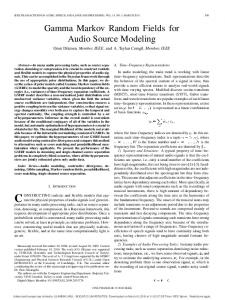
This distribution, which in our knowledge does not have a designated name, is a scale mixture of inverse Gamma distributions where the scaling function is also inverse Gamma. The transition kernel p(vk |vk−1 ) has positive correlation for various shape parameters az and a. The absolute value of az and a control the strength of the correlation and the ratio az /a controls the skewness. For az /a < 1 ( az /a > 1), the probability mass is shifted towards the interval vk < vk−1 ( vk > vk−1 ) hence, typical trajectories from a IGMC will exhibit a systematic negative (positive) drift. Using an exactly analogous construction, we define a Gamma-Markov chain (GMC) as z1 ∼ G(z1 ; az , (bz az )−1 ), λk |zk ∼ G(λk ; aλ , (zk aλ )−1 ), zk+1 |λk ∼ G(zk+1 ; az , (λk az )−1 ). The effective transition kernel has a very similar expression as in Eq.3. Example 1, Nonstationary Gaussian Process: We define a non-stationary Gaussian process {yk }k=1,2,... by drawing the variances {vk }k=1,2,... from an IGMC and drawing yk |vk ∼ N (yk ; 0, vk ) In Figure 1(a)-top, we show a realisation of v1:K from the IGMC, labelled as “true” and generate y1:K conditionally Figure 1(a)-bottom. Given a realisation y1:K , we can estimated the posterior variance hvk |y1:K i. In this case, inference is carried out with variational Bayes as will be detailed in section 3. Example 2, Nonhomogeneous Poisson Process: We partition an interval I on the real line into small disjoint regions Rk of area L such that I = ∪K k=1 Rk . We assume that the unknown intensity function of the process is piecewise constant and has the value λk on region Rk . The intensity function {λk }k=1,2,... is drawn according to a GMC. The number points in Rk , given the intensity function, is denoted by the Poisson random variable ck |λk ∼ PO(ck ; λk L) To generate a realisation from the Poisson process, we can uniformly draw ck points in each region Rk . In Figure 1(b), we show a realisation from the model. Given the number of events in each region Rk , we can estimate the value of the intensity function on Rk by calculating hλk |c1:K i. 2.2
(Inverse) Gamma Markov Random Fields – (I)GMRF
We have defined the IGMC and GMC in the previous section using conditional distributions. An alternative but equivalent factorisation, that encodes the same distribution but corresponds to Y −1 −1 p(z, v) ∝ ψ(b−1 φ(vk−1 ; a + az )φ(zk−1 ; a + az )ψ(azk−1 , vk−1 )ψ(az vk−1 , zk+1 ) z , az z1 ) k
where we specify singleton potentials φ and pairwise potentials ψ as φ(ξ; α) = exp((α + 1) log ξ)
ψ(ξ, η) = exp(−ξη)
Generalising this to a general undirected graph with vertex set V and undirected edge set E, we define an IGMRF on ξ = {ξi }i∈V by a set of connection weights a = {ai,j }(i,j)∈E for i, j ∈ V and i 6= j p(ξ; a) =
X Y 1 Y 1 ∗ pa (ξ) φ(ξi−1 ; ai,j ) ψ(ξi−1 , (ai,j /2)ξj−1 ) ≡ Za Z a j i∈V
(i,j)∈E
(4)
20
150 True VB
True VB k
100
10
λ
vk
15
50
5 0
0
200
400
600
800
0
1000
10
1 0.8
5 k
c
yk
0.6 0
0.4 −5 −10
0.2 0
200
400
600 k
800
0
1000
0
0.2
(a)
0.4
0.6 Arrival time
0.8
1
(b)
Fig. 1. Synthetic examples generated from the model. The thick line shows the result of the variational inference(a) Non-stationary Gaussian Process. (a-Top) a typical draw of v1:K from the IGMC bz = 1, a = az = 100. (a-Bottom) Draw from the Gaussian process y1:K given v1:K . (b) Non-homogeneous Poisson Process. (b-Top) a typical draw from the GMC with bz = 10, a = az = 100 and frame length µ(Rk ) = L = 0.001. (b-Bottom) Number of events in each Rk .
wherePφ and ψ are defined above. A GMRF is defined similarly by the potentials φ(ξi ; j ai,j ) and ψ(ξi , (ai,j /2)ξj ) but with φ(ξ; α) = exp((α − 1) log ξ).
3
Inference
Exact inference in random fields is in general intractable and various numerical methods have been developed, based on sampling (Monte Carlo-stochastic) or analytic approximation (Variational-deterministic). Here, we focus on a particularly simple variational algorithm (mean field - variational Bayes [1, 13]) – but application of Monte Carlo methods, such as the Gibbs sampler [7] is algorithmically very similar[2]. Variational methods have been applied extensively, notably in machine learning for inference in large models. While lacking theoretical guarantees of Monte Carlo approaches, variational methods have been viable alternatives in several practical situations where only a fixed amount of CPU budget is available. The main idea in variational Bayes is to approximate a target distribution P ≡ p∗ (ξ)/Z (such as the IGMRF defined in Eq.(4)) with a simple distribution Q. The variational distribution Q is chosen such that its expectations can be obtained easily, Q preferably in closed form. One such distribution is a factorised one Q(ξ) = i∈V Qi (ξi ). An intuitive interpretation of mean field method is minimising the KL divergence with respect to (the parameters of) Q where KL(Q||P) = hlog QiQ − hlog p∗ /Za iQ . Using non-negativity of KL, one can obtain a lower bound on log-normalisation constant log Za ≥ hlog p∗ iQ − hlog QiQ
(5)
The maximisation of this lower bound is equivalent to finding the “nearest” Q to P in terms of KL divergence. Whilst the solution is in general not available in closed form, it can be easily shown, e.g. see [13], that each factor Qi of the optimal
(a)
(b)
(c)
(d)
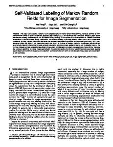
Fig. 2. Various IGMRF topologies as priors for time frequency energy distributions. White nodes (placed always on a rectangular grid) correspond to vν,τ where the vertical and horizontal axis corresponds to the frequency band index ν and time index τ respectively. Gray nodes correspond to the auxiliary variables z. (a)-(d) vertical, horizontal, band, grid.
approximating distribution should satisfy the following fixed point equation ³ ´ Qi ∝ exp hlog p∗ iQ−i (6) where Q−i ≡ Q/Qi , that is the joint distribution of all factors excluding Qi . Hence, the mean field approach leads to a set of (deterministic) fixed point equations that need to be iterated until convergence. For a MRF, this fixed point expression is efficient to evaluate since it depends only on the neighbouring variables j ∈ N (i). Finally, for conjugate models the factors are available in (t) (t) (t) closed form; for example IGMRF leads to the factors Qi (ξi ) = IG(ξi ; αi , βi ) with X X ® (t) (t) αi = θα,i + ai,j βi−1 = θβ,i + ai,j ξj−1 Q(t−1) j∈N (i)
j∈N (i)
j
Here, θα,i and θβ,i denote the data contributions when a IGMRF is used as a prior where some of the ξ are observed via a conjugate observation model. For example, in the conditionally Gaussian observation model of section 2 we have θα,i = 1/2 and θβ,i = yi2 /2. Similarly, the Poisson model with a GMRF prior has θα,i = ci and θβ,i = L. 3.1
Simulation Experiments
In Figure 1, we show the results of variational inference for two synthetic examples. In the following, we will illustrate the IGMRF model used as a prior for time-frequency energy distributions of nonstationary sources. Linear time-frequency representations decompose a signal y(t) as a linear P decomposition of form y(t) = (ν,τ ) s(ν,τ ) fν,τ (t) where s(ν,τ ) is the expansion coefficient corresponding to the basis function fν,τ (t). Somewhat succinctly we can write y = F s, where the collection of basis functions is denoted by a matrix F where each column corresponds to a particular fν,τ . The well known Gabor representation or modified cosine transform (MDCT) have this form and can be computed using fast transforms where τ corresponds to time and ν corresponds to frequency. In the sequel, we will impose a conditionally Gaussian prior on transform coefficients N (s(ν,τ ) ; 0, v(ν,τ ) ) where the covariance structure will be drawn from a IGMRF.
Denoising: In the first experiment, we illustrate the denoising performance of 4 MRF topologies on a set of 5 audio clips (speech, piano, guitar, perc1, perc2) in 3 different noise conditions low, medium, high. We transform each clip via MDCT to strue (ν,τ ) and add independent white Gaussian noise with variance r ∼ IG(r; ar , br ) to obtain x(ν,τ ) . Note that since MDCT is an orthonormal linear transform, we could have added noise in time domain and the noise characteristics would have remained unaltered. As inference engine, we use variational Bayes. The task of the inference algorithm is to infer the latent source coefficients s(ν,τ ) by integrating out the noise variance r and the IGMRF variables ξ. The optimisation of MRF parameters a is carried out by the Newton method where we maximise the lower bound in Eq.5. We assume homogeneous MRF structure where the coupling values are the same throughout the network 4 . The signal to noise ratio of reconstructions and inference results are given in Figure 3-(a). The SNR results do not show big variations across topologies, with the grid model consistently providing good reconstruction, especially in high and medium noise conditions. We note that SNR may not be the best metric to measure perceptual quality and the reader is invited to listen to the audio examples provided online at http://www.cmpe.boun.edu.tr/∼dikmen/ICA07/. In informal subjective listening tests, we perceive a somewhat better reconstruction quality with the grid topology. Source Separation: In the second experiment, we illustrate the viability of the approach on a single channel separation task with j = 1 . . . J sources. At each time-frequency location k ≡ (ν, τ ), the generative model is vj ∼ IGMRFj , sk,j ∼ PJ N (sk ; 0; vk,j ), xk = j=1 sk,j In this scenario, the reconstruction equations have −1 a particularly simple form. Given the variance estimate Vk,j = h1/vk,j i at k, we define a positive quantity, P which we shall name as responsibility also know as 0 filter factors, κ = V /( k,j k,j j 0 Vk,j ), where by construction 0 < κj for all j and P κ ≤ 1. It turns out that the sufficient statistics can be compactly written as j j hsk,j i = κk,j xk
2 ® sk,j = Vk,j (1 − κk,j ) + κ2k,j x2k
We illustrate this approach to separate a piano sound into its constituent components. We assume that J = 2 components are generated independently by two IGMRF models with vertical and horizontal topology. In figure 3-(b), we observe that the model is able to separate transients and harmonic components. 3.2
Discussion
We have introduced a conjugate gamma Markov random field model for modelling nonstationary sources. The conjugacy makes it possible to design fast inference algorithms in a straightforward way. The simple MRF topologies considered here are quite generic, yet provide good results without any hand tuned parameters. One can envision more structured models with a larger set of parameters to 4
In (a) (vertical), each white node is connected to two gray nodes with anorth or asouth and in (b) (horizontal) with awest or aeast . The grid topology (d) has couplings in four directions and in (c) (band), we use a single a.
Xorg
Shor
Sver
SNR
20 band ver hor grid
15
medium 10 speech
Frequency Bin (ν)
low
high piano
guitar
perc1
perc2
Time (τ) Audio Signals (a) (b) Fig. 3. (a) Signal-to-Noise ratio results for reconstructions obtained from the audio clips in low, medium,high noise conditions. (b) Single channel Source Separation example, left to right, log-MDCT coefficients of the original signal and reconstruction with horizontal and vertical IGMRF models.
capture physical reality, certainly for acoustical signals. We are currently investigating further applications such as restoration, transcription or tracking time varying intensity functions.
References 1. H. Attias. Independent factor analysis. Neural Computation, 11(4):803–851, 1999. 2. A. T. Cemgil, C. Fevotte, and S. J. Godsill. Variational and Stochastic Inference for Bayesian Source Separation. Digital Signal Processing, in Print, 2007. 3. A. Cichocki and S. I. Amari. Adaptive Blind Signal and Image Processing: Learning Algorithms and Applications. Wiley, revised version edition, April 2003. 4. C. F´evotte, L. Daudet, S. J. Godsill, and B. Torr´esani. Sparse regression with structured priors: Application to audio denoising. In Proc. ICASSP, Toulouse, France, May 2006. 5. Aapo Hyv¨ arinen, Juha Karhunen, and Erkki Oja. Independent Component Analysis. John Wiley & Sons, New York, NY, 2001. 6. K. H. Knuth. Bayesian source separation and localization. In SPIE’98: Bayesian Inference for Inverse Problems, pages 147–158, San diego, Jul. 1998. 7. J. S. Liu. Monte Carlo strategies in scientific computing. Springer, 2004. 8. D. J. C. MacKay. Information Theory, Inference and Learning Algorithms. Cambridge University Press, 2003. 9. J. Miskin and D. Mackay. Ensemble learning for blind source separation. In S. J. Roberts and R. M. Everson, editors, Independent Component Analysis, pages 209– 233. Cambridge University Press, 2001. 10. M. Reyes-Gomez, N. Jojic, and D. Ellis. Deformable spectrograms. In AI and Statistics Conference, Barbados, 2005. 11. D. B. Rowe. A Bayesian approach to blind source separation. Journal of Interdisciplinary Mathematics, 5(1):49–76, 2002. 12. N. Shepard, editor. Stochastic Volatility, Selected Readings. Oxford University Press, 2005. 13. M. Wainwright and M. I. Jordan. Graphical models, exponential families, and variational inference. Technical Report 649, Department of Statistics, UC Berkeley, September 2003. 14. P. J. Wolfe, S. J. Godsill, and W.J. Ng. Bayesian variable selection and regularisation for time-frequency surface estimation. Journal of the Royal Statistical Society, 2004. 15. R. L. Wolpert and K. Ickstadt. Poisson/gamma random field models for spatial statistics. Biometrica, 1998.