Chapter 12 in S.W. Ellacott, J.C. Mason & I.J. Anderson (eds.) MATHEMATICS OF NEURAL NETWORKS Models, Algorithms and Applications Kluwer Academic Publishers, Boston, 89-94, 1997
CONSTANT FAN-IN DIGITAL NEURAL NETWORKS ARE VLSI-OPTIMAL † Valeriu Beiu ‡ Los Alamos National Laboratory, Division NIS-1, MS D466 Los Alamos, New Mexico 87544, USA E-mail:
[email protected]
The paper presents a theoretical proof revealing an intrinsic limitation of digital VLSI technology: its inability to cope with highly connected structures (e.g., neural networks). We are in fact able to prove that efficient digital VLSI implementations (known as VLSI-optimal when minimising the AT 2 complexity measure — A being the area of the chip, and T the delay for propagating the inputs to the outputs) of neural networks are achieved for small–constant fan-in gates. This result builds on quite recent ones dealing with a very close estimate of the area of neural networks when implemented by threshold gates, but it is also valid for classical Boolean gates. Limitations and open questions are presented in the conclusions. Keywords: neural networks, VLSI, fan-in, Boolean circuits, threshold circuits, Fn,m functions.
1. Introduction In this paper a network will be considered an acyclic graph having several input nodes (inputs) and some (at least one) output nodes (outputs). The nodes are characterised by fan-in (the number of incoming edges — denoted by ∆) and fan-out (the number of outgoing edges), while the network has a certain size (the number of nodes) and depth (the number of edges on the longest input to output path). If with each edge a synaptic weight is associated and each node computes the weighted sum of its inputs to which a nonlinear activation function is then applied (artificial neuron), the network is a neural network (NN): (1) Z = (z , …, z ) ∈ IRn, k = 1, … , m, and f (Z ) = σ ( ∑ n − 1 w z + θ) , k
0
n−1
k
i=0
i
i
with wi ∈IR the synaptic weights, θ ∈IR known as the threshold, and σ a non-linear activation function. If the non-linear activation function is the threshold (logistic) function, the neurons are threshold gates (TGs) and the network is just a threshold gate circuit (TGC) computing a Boolean function (BF). The cost functions associated to a NN are depth and size. These are linked to T ≈ depth and A ≈ size of a VLSI chip. Unfortunately, NNs do not closely follow these proportionalities as: the area of the connections counts [2, 3, 9]; the area of one neuron is related to its associated weights. That is why the size and depth complexity measures are not the best criteria for ranking different solutions when going to silicon [11]. Several authors have taken into account the fan-in [1, 9, 10, 12], the total number of connections, the total number of bits needed to represent the weights [8, 15]
† This research has been financed by the Commission of the European Communities under contract ERBCHBICT941741. The scientific responsibility is assumed by the author. ‡ On leave of absence from “Politehnica” University of Bucharest, Department of Computer Science, Spl. Independentei 313, RO-77206 Bucharest, România.
Beiu: Chapter 12
Constant Fan-in Digital Neural Networks are VSLI-optimal
90
or even more precise approximations like the sum of all the weights and thresholds [2-7]: area ∝
∑ all neurons
∑ in=−01 | wi | + | θ | .
(2)
An equivalent definition of ‘complexity’ for a NN is ∑ ni =−01 w2i [16]. It is worth mentioning that there are also several sharp limitations for VLSI implementations like: (i) the maximal value of the fan-in cannot grow over a certain limit; (ii) the maximal ratio between the largest and the smallest weight. For simplification, in the following we shall consider only NNs having n binary inputs and k binary outputs. If real inputs and outputs are needed, it is always possible to quantize them up to a certain number of bits such as to achieve a desired precision. The fan-in of a gate will be denoted by ∆ and all the logarithms are taken to base 2 except mentioned otherwise. Section 2 will present previous results for which proofs have already been given [2-7]. In section 3 we shall prove our main claim while also showing several simulation results.
2. Background A novel synthesis algorithm evolving from the decomposition of COMPARISON has recently been proposed. We have been able to prove that [2, 3]: Proposition 1 The computation of COMPARISON of two n-bit numbers can be realised by a ∆ary tree of size O (n / ∆) and depth O(logn / log∆) for any integer fan-in 2 ≤ ∆ ≤ n. A class of Boolean functions IF∆ having the property that ∀f∆ ∈ IF∆ is linearly separable has afterwards been introduced as: “the class of functions f∆ of ∆ input variables, with ∆ even, def f∆ = f∆ (g∆/2−1,e∆/2−1,…,g0,e0), and computing f∆ = ∨j∆=/ 02 − 1 gj ∧ (∧k∆=/ 2j +− 11 ek) .” By convention, we con def α−1 sider ∧i = α ei = 1. One restriction is that the input variables are pair-dependent, meaning that we can group the ∆ input variables in ∆ / 2 pairs of two input variables each: (g∆/2−1, e∆/2−1) ,…, (g0, e0), and that in each such group one variable is ‘dominant’ (i.e., when a dominant variable is 1, the other variable forming the pair will also be 1): IF∆ = f∆ | f∆:{(0,0),(0,1),(1,1)}∆ / 2 → {0,1}, ∆ / 2 ∈ IN,∗ def
f∆ =∨j∆=/ 02 − 1 gj ∧ (∧k∆=/ 2j+−1 1 ek), gi ⇒ ei, i=0,1,…,∆ / 2−1 . Each f∆ can be built starting from the previous one f∆−2 (having a lower fan-in) by copying its synaptic weights; the constructive proof has led to [5]: Proposition 2 The COMPARISON of two n-bit numbers can be computed by a ∆-ary tree neural network with polynomially bounded integer weights and thresholds (≤ nk) having size O (n / ∆) and depth O(logn / log∆) for any integer fan-in 3 ≤ ∆ ≤ logkn.
For a closer estimate of the area we have used equation (2) and proved [5]: Proposition 3 The neural network with polynomially bounded integer weights (and thresholds) computing the COMPARISON of two n-bit numbers occupies an area of O (n ⋅ 2∆ / 2/ ∆) for all the values of the fan-in (∆) in the range 3 to O ( logn) . The result presented there is: AT 2 (n,∆) ≅
nlog2n ⋅ 2∆ / 2 2∆ / 2 8n∆ − 6n − 5∆ log2n ⋅ ⋅ = O 2 ∆ ∆−2 log2∆ ∆ log ∆
(3)
Beiu: Chapter 12
Constant Fan-in Digital Neural Networks are VSLI-optimal
91
and for ∆ = logn this is the best (i.e., smallest) one reported in the literature. Further, the synthesis of a class of Boolean functions Fn,m —functions of n input variables having m groups of ones in their truth table [13]— has been detailed [4]: Proposition 4 Any function f ∈ Fn,m can be computed by a neural network with polynomially bounded integer weights (and thresholds) of depth O (log(mn) / log∆) and size O (mn / ∆), and occupying an area of O (mn ⋅ 2∆ / ∆) if 2m ≤ 2∆ for all the values of the fan-in (∆) in the range 3 to O ( logn) . More precisely we have: T (n,m,∆) A (n,m,∆)
logn − 1 logm + 1 log(mn) = + log∆ = O log∆ log ∆ − 1 4n ⋅ 2∆ 5(n − ∆) ⋅ 2∆ / 2 2m − 1 + < 2m ⋅ +∆⋅ ∆(∆ − 2) ∆ ∆−1
and mn ⋅ 2∆ = O ∆
which leads to: (4) mn ⋅ log2(mn) ⋅ 2∆ = O . ∆ ⋅ log2∆ For 2m > 2∆ the equations are much more intricate, while the complexity values for area and for AT 2 are only reduced by a factor (equal to the fan-in [6, 7]). If we now suppose that a feedforward NN of n inputs and k outputs is described by m examples, it can be directly constructed as simultaneously implementing k different functions from Fn,m [4, 6, 7]: Proposition 5 Any set of k functions f ∈ Fn,i , i = 1, 2, … , m, i ≤ m ≤ 2∆−1 can be computed by a neural network with polynomially bounded integer weights (and thresholds) having size O (m (2n+k) / ∆), depth O (log(m n) / log∆) and occupying an area of O (m n ⋅ 2∆ / ∆ + mk) if 2m ≤ 2∆, for all the values of the fan-in (∆) in the range 3 to O ( logn) . AT 2 (n,m,∆)
The architecture has a first layer of COMPARISONs which can either be implemented using classical Boolean gates (BGs) or — as it has been shown previously — by TGs. The desired function can be synthesised either by one more layer of TGs, or by a classical two layers AND-OR structure (a second hidden layer of AND gates — one for each hypercube), and a third layer of k OR gates represents the outputs. For minimising the area some COMPARISONs could be replaced by AND gates (like in a classical disjunctive normal form implementation).
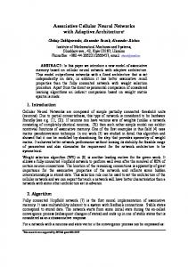
3. Which is the VLSI-Optimal Fan-In ? Not wanting to complicate the proofs, we shall determine the VLSI-optimal fan-in when implementing COMPARISON (in fact an Fn,1 function) for which the solution was detailed in Propositions 1 to 3. The same result is valid for Fn,m functions as can be intuitively expected either by comparing equations (3) and (4), or because: the delay is determined by the first layer of COMPARISONs; while the area is mostly influenced by the same first layer of COMPARISONs (the additional area for the implementing the symmetric ‘alternate addition’ [4] can be neglected). For a better understanding we have plotted equation (3) in Figure 1. Proposition 6 The VLSI-optimal (which minimises the AT 2) neural network which computes the COMPARISON of two n-bit numbers has small-constant fan-in ‘neurons’ with small-constant bounded weights and thresholds.
Beiu: Chapter 12
Proof:
Constant Fan-in Digital Neural Networks are VSLI-optimal
92
Starting from the first part of equation (3) we can compute its derivative: d (AT 2) 2∆ / 2 log2n = 2 × 8n∆3log∆ − 22n∆2log∆ + 12n∆log∆ − 5∆3log∆ + d∆ ∆ (∆−2)2log3∆ + 10∆2log∆ −
16 2 24 24 10 2 n∆ log∆ + n∆log∆ − nlog∆ + ∆ log∆ − ln2 ln2 ln2 ln2
− 32 n∆2 + 88 n∆ − 48 n + 20 ∆2 − 40 ∆ ln2 ln2 ln2 ln2 ln2 which — unfortunately — involves transcendental functions of the variables in an essentially non-algebraic way. If we consider the simplified ‘complexity’ version of equation (3) we have: nlog2n ⋅ 2∆ / 2 2∆ / 2 ln2 1 2 = ⋅ − − 2 2 2 ∆ ∆ ln ∆ ∆ log ∆ ∆ log ∆ which when equated to zero leads to ln∆ (∆ ln2 − 2) = 4 (also a transcendental equation). This has ∆ = 6 as ‘solution’ and as the weights and the thresholds are bounded by 2∆ / 2 (Proposition 4) the proof is concluded. q
d (AT 2) d ≅ d∆ d∆
The proof has been obtained using several successive approximations: neglecting ceilings, using a ‘simplified’ complexity estimate. That is why we present in Figure 2 exact plots of the AT 2 measure which support our previous claim. It can be seen that the optimal fan-in ‘constantly’ lies between 6 and 9 (as ∆optim = 6…9, one can minimise the area by using COMPARISONs only if the group of ones has a length of α ≥ 64 — see [4-7]). Some plots in Figure 2 are also including a TG-optimal solution denoted by SRK [14] and the logarithmic fan-in solution (∆ = logn) denoted B_lg [5].
4. Conclusions This paper has presented a theoretical proof for one of the intrinsic limitations of digital VLSI technology: there are no ‘optimal’ solutions able to cope with highly connected structures. For doing that we have proven the contrary, namely that constant fan-in NNs are VLSI-optimal for digital architectures (either Boolean or using TGs). Open questions remain concerning ‘if’ and ‘how’ such a result could be used for purely analog or mixed analog/digital VLSI circuits.
6
4
x 10
x 10
6
10
5
8 6 AT^2
AT^2
4 3 2
2
0 1000
0 60
800 600 n
40 400
n
20
20
20
15
200
(a)
4
1
15
10 0
10
5 0
fan-in
(b)
0
5 0
fan-in
Figure 1. The AT 2 values of COMPARISON —plotted as a 3D surface— versus the number of inputs n and the fan-in ∆ for: (a) many inputs n ≤ 1024 (4 ≤ ∆ ≤ 20); and (b) few inputs n ≤ 64 (4 ≤ ∆ ≤ 20). It can be very clearly seen that a ‘valley’ is formed and that the ‘deepest’ points constantly lie somewhere between ∆minim = 5 and ∆maxim = 10.
Beiu: Chapter 12
Constant Fan-in Digital Neural Networks are VSLI-optimal
93
Acknowledgements This research work has been started while Dr. Beiu was with the Katholieke Universiteit Leuven, Belgium, and has been supported by a grant from the Concerted Research Action of the Flemish Community entitled: “Applicable Neural Networks.” The research has been continued under the Human Capital and Mobility programme of the European Community as an Individual Research Training Fellowship ERB4001GT941815: “Programmable Neural Arrays,” u nd er con tract ERBCHBICT941741. The scientific responsibility is assumed by the author, who is on leave of absence from the “Politehnica” University of Bucharest, România. 14000
7000 SRK
B_4
B_16
B_6
12000
6000
10000
5000
B_8
4000
B_7
8000 AT^2
AT^2
B_lg B_5
6000
B_9
3000
B_8 4000
2000
2000
1000
0 0
(a)
5
10
15
20
25
30
35
n
0 0
(b)
10
15
20
25
30
35
n
5
3.5
5
4
x 10
14 SRK
x 10
B_6
B_16
3
B_4
12 B_7
2.5
10 B_9
2
AT^2
AT^2
B_8
8
B_5
1.5
6
1
4
B_8 B_lg
0.5
2
0 0
(c)
50
100
150 n
200
250
300
0 0
(d)
6
2
50
100
150 n
200
250
300
5
x 10
SRK
B_16
8
B_4
1.8
x 10
B_6
7
6
B_7 B_9
5
B_8
1.6 1.4
AT^2
AT^2
1.2 B_5
1 0.8
B_lg
0.6
4
3
B_8
2
0.4 1
0.2
(e)
0 200
300
400
500
600
700 n
800
900
1000
1100
(f)
0 200
300
400
500
600
700
800
900
1000
1100
n
Figure 2. The AT 2 values of COMPARISON for different number of inputs n and fan-in ∆ (B_∆): (a) for 4 ≤ ≤ n ≤ 32 including the SRK [14] solution; (b) detail showing the optimum fan-in for the same interval (4 ≤ n ≤ 32); (c) for 32 ≤ n ≤ 256 including the SRK [14] solution; (d) detail showing the optimum fan-in for the same interval (32 ≤ n ≤ 256); (e) for 256 ≤ n ≤ 1024 including the SRK [14] solution; (f) detail showing the optimum fan-in for the same interval (256 ≤ n ≤ 1024).
Beiu: Chapter 12
Constant Fan-in Digital Neural Networks are VSLI-optimal
94
References [1] Y.S. Abu-Mostafa, Connectivity Versus Entropy, in: Neural Information Processing Systems, ed. D.Z. Anderson (Amer. Inst. of Physics, New York, 1988) 1-8. [2] V. Beiu, J.A. Peperstraete, J. Vandewalle and R. Lauwereins, Efficient Decomposition of COMPARISON and Its Applications, in: ESANN’93, ed. M. Verleysen (Dfacto, Brussels, 1993) 45-50. [3] V. Beiu, J.A. Peperstraete, J. Vandewalle and R. Lauwereins, COMPARISON and Threshold Gate Decomposition, in: MicroNeuro’93, eds. D.J. Myers and A.F. Murray (UnivEd Tech. Ltd., Edinburg, 1993) 83-90. [4] V. Beiu, J.A. Peperstraete, J. Vandewalle and R. Lauwereins, Learning from Examples and VLSI Implementation of Neural Networks, in: Cybernetics and System Research ’94, ed. R. Trappl (World Scientific Publishing, Singapore, 1994) 1767-1774. [5] V. Beiu, J.A. Peperstraete, J. Vandewalle and R. Lauwereins, Area–Time Performances of Some Neural Computations, in: SPRANN’94, eds. P. Borne, T. Fukuda and S.G. Tzafestas (GERF EC, Lille, 1994) 664-668. [6] V. Beiu and J.G. Taylor, VLSI Optimal Neural Network Learning Algorithm, in: Artificial Neural Nets and Genetic Algorithms, eds. D.W. Pearson, N.C. Steele and R.F. Albrecht (Springer-Verlag, Vienna, 1995) 61-64. [7] V. Beiu and J.G. Taylor, Area-Efficient Constructive Learning Algorithms, in Proc. CSCS10, ed. I. Dumitrache (PUBucharest, Bucharest, 1995), 293-310. [8] J. Bruck and J. Goodman, On the Power of Neural Networks for Solving Hard Problems, in: Neural Information Processing Systems, ed. D.Z. Anderson (Amer. Inst. of Physics, New York, 1988) 137-143. [9] D. Hammerstrom, The Connectivity Analysis of Simple Associations –or– How Many Connections Do You Need, in: Neural Information Processing Systems, ed. D.Z. Anderson (Amer. Inst. of Physics, New York, 1988) 338-347. [10] H. Klaggers and M. Soegtrop, Limited Fan-In Random Wired Cascade-Correlation, in: MicroNeuro’93, eds. D.J. Myers and A.F. Murray (UnivEd Tech. Ltd., Edinburg, 1993) 79-82. [11] A.V. Krishnamoorthy, R. Paturi, M. Blume, G.D. Linden, L.H. Linden and S.C. Esener, Hardware Tradeoffs for Boolean Concept Learning, in WCNN’94, (Lawrence Erlbaum and INNS Press, Hillsdale, 1994) vol. 1/551-559. [12] D.S. Phatak and I. Koren, Connectivity and Performance Tredeoffs in the Cascade-Correlation Learning Architecture, IEEE Trans. on Neural Networks 5(6) (1994) 930-935. [13] N.P. Red’kin, Synthesis of Threshold Circuits for certain Classes of Boolean Functions, Kibernetica 5 (1970) 6-9. Translated in Cybernetics 6(5) (1973) 540-544. [14] K.-Y. Siu, V. Roychowdhury and T. Kailath, Depth-Size Tradeoffs for Neural Computations, IEEE Trans. on Computers 40(12) (1991) 1402-1412. [15] R.C. Williamson, ε–Entropy and the Complexity of Feedforward Neural Networks, in: Neural Information Processing Systems, eds. R.P. Lippmann, J.E. Moody and D.S. Touretzky (Morgan Kaufmann, San Mateo, 1991) 946-952. [16] B.-T. Zhang and H. Mühlenbein, Genetic Programming of Minimal Neural Networks Using Occam’s Razor, Technical Report: Arbeitspapiere der GMD 734, Schloß Birlinghoven, Sankt Augustin, Germany (1993).