consider a collected set of data measurements in traffic flow analysis [9], or in ... tain data, (2) a formal framework for solving systems of arithmetic constraints over ... For independent variables P(X ≤ x, Y ≤ y) = FX(x) × FY(y). ..... into two cdf-interval inequalities; then the cdf-constraints are transformed into ... −6x1 − 3x2 ≤ −4.
Constraint Reasoning with Uncertain Data using CDF-Intervals Aya Saad, Carmen Gervet and Slim Abdennadher German University in Cairo New Cairo City, Egypt {aya.saad, carmen.gervet, slim.abdennadher}@guc.edu.eg
Abstract. Interval coefficients have been introduced in OR and CP to specify uncertain data in order to provide reliable solutions to convex models. The output is generally a solution set, guaranteed to contain all solutions possible under any realization of the data. This set can be too large to be meaningful. Furthermore, each solution has equal uncertainty weight, thus does not reflect any possible degree of knowledge about the data. To overcome these problems we propose to extend the notion of interval coefficient by introducing a second dimension to each interval bound. Each bound is now specified by its data value and its degree of knowledge. This is formalized using the cumulative distribution function of the data set. We define the formal framework of constraint reasoning over this cdf-intervals. The main contribution of this paper concerns the formal definition of a new interval arithmetic and its implementation. Promising results on problem instances demonstrate the approach.
1 Introduction Interval coefficients have been introduced in Operations Research and Constraint Programming to specify uncertain data in order to provide reliable solutions to convex models. They are at the heart of paradigms such as robust optimization [3, 12] in Operations Research as well as mixed CSP [8], reliable constraint reasoning [15, 16], and quantified CSP [17] in Constraint Programming. These paradigms specify erroneous and incomplete data using uncertainty sets that denote a deterministic and bounded formulation of an ill-defined data. To remain computationally tractable, the uncertainty sets are approximated by convex structures such as intervals (extreme values within the uncertainty set) and interval reasoning can be applied ensuring effective computations. The concept of convex modeling was coined to formalize the idea of enclosing uncertainty sets and yield reliable solutions; i.e guaranteed to contain any solution produced by any possible realization of the data [2, 5, 16]. As a result, the outcome of such systems is a solution set that can be refined when more knowledge is acquired about the data, and does not exclude any potential solution. The benefits of these approaches are that they deal with real data measurements, produce robust/reliable solutions, and do so in a computationally tractable manner. However, the solution set can sometimes be too large to be meaningful since it encloses all solutions that can be constructed using the data intervals. Furthermore each solution derived has equal uncertainty weight, thus does not reflect any possible degree of knowledge about the data. For instance,
consider a collected set of data measurements in traffic flow analysis [9], or in image recognition [7], the data is generally ill-defined but some data values can occur more than others or have a darker shade of grey (hence greater degree of knowledge or certainty). This quantitative information is available during data collection, but lost during the reasoning because not accounted for in the representation of the uncertain data. As a consequence it is not available in the solution set produced. Mainly reliable models offer reliability and robustness, tractable models, but do not account for quantitative information about the data. This paper addresses this problem. Basically we extend the interval data models with a second dimension: a quantitative dimension added to the measured input data. The main idea introduced in this paper is to show that we can preserve the tractability of convex modeling while enriching the uncertain data sets with a representation of the degree of knowledge available. Our methodology consists of building data intervals employing two dimensional points as extreme values. We assume that with each uncertain data value comes its frequency of occurrence or density function. We then compute the cumulative distribution function (cdf) over this function. The cdf is an aggregated quantitative measurement indicating for a given uncertain value, the probability that the actual data value lies before it. It has been used in different models under uncertainty to analyze the distribution of data sets (e.g. [14] and [10]). It enjoys three main properties that fit an interval representation of data uncertainty: i) the cdf is a monotone, non decreasing function like arithmetic ordering, suitable for interval computations and pruning, ii) it directly represents the aggregated probability that a quantity lies within bounds, thus showing the confidence interval of this uncertain data, iii) it brings flexibility to the problem modeling assumptions (e.g. by choosing the data value bounds based on the cdf values, or its sought confidence interval). We introduce the concept of cdf-intervals to represent such convex sets, following the concept of interval coefficients. This requires the decision variables to range over cdf-intervals as well. Basically, in our framework, the elements of a variable’s domain are points in a 2D-space, the first dimension for its data value, the second for its aggregated cdf value. It is defined as a cdf-interval specified by its lower and upper bounds. A new domain ordering is defined within the 2D space. This raises the question of performing arithmetic computations over such variables to infer bound consistency. We define the constraint domain over which the calculus in this new domain structure can be performed, including the inference rules. This paper contains the following contributions: (1) a new representation of uncertain data, (2) a formal framework for solving systems of arithmetic constraints over cdf-intervals, (3) a practical framework including the inference rules within the usual fixed point semantics, (4) an application to interval linear systems. The paper is structured along the contributions listed hereabove.
2 Basic Concepts This section recalls basic concepts we use to characterize the degree of knowledge, and introduces our notations. These definitions can be found in [10].
2.1 Cumulative Distribution Function Throughout this paper we assume independence of data. Definition 1 (density function). Given a data set {N1 , ..., Nn }, with available information regarding the occurrence of each data item. The density function f (x) of a data item x, is defined over the population size, m, by: number of occurrences of valueN x (1) m The cumulative distribution function cdf of a given value, defines its accumulated density so far. It does not assume any specific distribution function, but follows that of the density function. f (x) =
Definition 2 (cumulative distribution function). Given an item value x, with density function f (x), and an unknown variable (commonly referred to as the real-valued random variable) X, the cdf of x is the function: X F X (x) = P(X ≤ x) = f (x) (2) X≤x
The cdf ranges over the interval [0,1]. Property 1. Every cdf is monotone, and right continuous. In other words, the cdf value of a point is the density value of that point in addition to the sum of frequencies of all preceding points, with smaller item value. As illustrated in fig. 1 the cdf associated with a density function is always increasing until it reaches the point of stability ’1’ where the curve remains constant. All the data population resides between two points having cdf values ’0’ and ’1’ with an average step height equivalent to (m/n), where n is the number of distinct values in the data set and m is the size of its population. The cdf expresses the distribution of the data in an aggregated manner. 2.2 Joint Cumulative Distribution Function Operations can be performed on cdfs but carry a different interpretation than operations over standard arithmetic calculus since they relate to probabilities. The joint operation is essential to our solver and is recalled below. The joint cdf is the cdf that results from superimposing two variables with a relation, each exerting a cdf on its own. Definition 3 (Joint CDF). Given two random variables X and Y 1 F XY (x, y) = P(X ≤ x, Y ≤ y)
(3)
For independent variables P(X ≤ x, Y ≤ y) = F X (x) × FY (y). Definition 4 (Joint CDF over bounded intervals). When X and Y are bounded intervals; i.e. X ∈ [a, b] and Y ∈ [c, d], the joint CDF is defined by: P(a ≤ X ≤ b, c ≤ Y ≤ d) = F XY (b, d) − F XY (a, d) − F XY (b, c) + F XY (a, c)
(4)
The joint cdf F XY of two variables X and Y is used extensively in the computation of the cdf resulting from any operation between the variables. 1
Recall that a random variable maps an event to values, e.g. event that X ≤ x.
(a)
(b)
Fig. 1. constructing the data interval bounds
2.3 Notations We assume that a data takes its value in the set of real numbers R, denoted by a,b,c. A cdf value F X (x) is associated to the uncertainty curve of a given point p. For simplicity, F X (x) is noted F xp , i.e. the cdf value of an uncertain data p at value x. We have p x ∈ R × [0, 1] with coordinates (x, F xp ). Data points are denoted by p, q, r possibly subscripted by a data value. Variables are denoted by X, Y, Z and take their value in U = R × [0, 1]. Intervals of elements from U are denoted I, J, K. We denote F I the approximated linear curve relative to the cdf curve inbetween the bounds of I, and FaI the cdf value of the data value a plotted on the 2D-interval I.
3 Uncertain Data Representation Given a measured (also possibly randomly generated) data set denoting the population of an uncertain data, we construct our cdf-intervals as detailed in algorithm 1. procedure ConstructIntervalBounds(m, Arr[n], Freq[n]) 1: cdf[1] ← Freq[1]/m 2: for i = 2 to n do 3: cdf[i] ← (Freq[i]/m) + cdf[i − 1] 4: i = 1, 5: while (Freq[i] ≤ m/n) do { m/n is the average step value} 6: i←i+1 7: lowerbound ← (Arr[i], cdf[i]) 8: upperbound ← (cdf−1 [0.98], 0.98)
Algorithm 1: data interval bounds construction
The algorithm runs in O(n) where n is the number of distinct values in the data set. It receives three parameters: the size of the data population, m, a sorted list (ascending
order) of the distinct measured data, and a list of their corresponding frequencies. Both lists are of the same size n. The algorithm first computes the cdf in a cumulative manner. The turning points are then extracted by recording the data value having a density less than the average step value (m/n) and the value with cdf equal to 98%. Fig.1 illustrates an example of an interval data construction. For a data set size n = 11, and a population size m = 30, Arr[n] = [12, 15, 18, 21, 24, 27, 30, 33, 36, 39, 42], and its corresponding frequencies Freq[n] = [1, 3, 6, 5, 3, 4, 2, 2, 2, 1, 1], the computed cdf-interval has the following bounds [(15, 0.13), (39.6, 0.98)]. 3.1 Interpretation of the confidence interval [pa , pb ] Consider the practical meaning of the interval [pa , pb ] that we have sought to obtain. This interval is built according to two main sources of information: 1) the monotony and non-decreasing properties of the cdf curve to account for degree of knowledge, 2) the extreme turning points over such a curve. Recall that the cdf curve indicates the aggregated distribution function of a data set. Plotting a point on this curve tells us what are the chances that the actual data value lies on or before this point. The extreme turning points we have considered are such that the lower bound indicates when the slope (thus frequency of occurrence over the population) increases more than the average; and the upper bound that of the cdf reaching a plateau. The measure of this upper bound has been associated with the cdf value of 98%. This corresponds to the distance of avr + 3σ when the distribution follows a normal distribution. Such interpretation is a conservative view that can be revised by the decision maker. It is also important to note the effectiveness of using the cdf as an indicator of degree of knowledge. Given a measurement of the data p such that (x, F xp ) is any point, we have the following due to F p monotone non-decreasing property: a ≤ x ≤ b,
Fap ≤ F xp ≤ Fbp
This implies that we can order (partially) points in this 2D-space U = R × [0, 1]. Thus we can construct an algebra over variables taking their value in this space. In particular, we can approximate the cdf curve associated with a data population by the linear (increasing or constant) slope between the two turning points. 3.2 Linear Approximation within I = [pa , pb ] Definition 5. For a given interval I = [pa , pb ], F xI is the projected approximated cdf value of p x onto F I (the cdf associated to the interval), we will denote p x ∈ I as p x = (x, F xI ) for any point lying within the I interval bounds such that: a < x < b, F xI =
FbI − FaI .(x − a) + FaI b−a
(5)
Property 2. Fap = FaI and Fbq = FbI Example 1. Fig. 2 illustrates the computation of F xI . We have I = [(18.6, 0.44), (27.8, 0.78)]. Given a data value x = 24 we compute its cdf F xI = 0.64, and obtain the point p x = (24, 0.64).
Fig. 2. F xI linear projection
4 cdf-Intervals Our approach follows real interval arithmetic. It adds a second dimension to each uncertain value, requiring us to define a new ordering among points in a two dimensional space, together with new inference rules. Consider a data population with its cdf curve. Create the set of points such that each points p x is specified by (x, F x ) ∈ R × [0, 1]. The set U = R × [0, 1] is a set of tuples partially ordered, and constitutes a poset with a unique greatest lower bound and least upper bound. Similarly to reliable computing methods the constraint system will produce a solution set as opposed to a solution point. The variables thus denote intervals within the cdf-interval structure and constraint processing needs to be extended to perform arithmetic operations within this algebraic structure. 4.1 cdf-Interval ordering 4 Definition 6 (Ordering over U, 4). Let p x = (x, F xp ), qy = (y, Fyq ) ∈ U, the ordering 4 is a partial order defined by: q
p x 4 qy ⇔ x ≤ y and F xp ≤ Fy
Example 2. Consider the three points p x = (1, 0.3), qy = (2, 0.5) and rz = (2, 0.1). We have p x 4 qy as well as rz 4 qy , but p x and rz are not comparable. A cdf-interval delimited by two points p x and qy is specified by the syntax [p x , qy ] such that p x 4 qy . One important task in interval reasoning is the computation of a new interval from arbitrary points or previous intervals, such that it describes the smallest interval containing a collection of elements. This is based on the meet and joint operators. Definition 7 (meet and join). Given the arithmetic ordering and meet and join operations over the reals (R, ≤, min, max) and the ordering of cdf values within ([0, 1], ≤
, min, max), the meet lub and join glb operators of two points p x and qy in U are defined by: q glb(p x , qy ) = (min(x, y), min(Flbp , Flb )) q
p lub(p x , qy ) = (max(x, y), max(Fub , Fub ))
(6)
where lb = min(x, y) and ub = max(x, y) The following property establishes the link between the partial ordering 4 and the pair (glb, lub) as actual meet and join. Property 3 (Consistency property). p x 4 qy ⇔ p x = glb(p x , qy ) p x 4 qy ⇔ qy = lub(p x , qy )
(7)
Fig. 3. glb and lub computation
Fig. 3 illustrates an example which computes glb and lub of two points p x = (1, 0.3) and qy = (2, 0.1). glb(p x , qy ) = (1, 0.05) and lub(p x , qy ) = (2, 0.6). 4.2 cdf Domains The key element to a cdf-Interval domain is the approximated cdf curve it lies on. However, to remain computationally tractable we do not maintain a full domain representation of the points defining the curve. Instead, we approximate the curve by a linear curve whose extreme points are the bounds of the interval. Elements of the interval domain lie on the linear curve. This leads to the following concept of cdf-Interval domain. Definition 8 (cdf-Domain). A cdf-Domain is a pair [pa , pb ] satisfying pa 4 pb and denoting the set: {p x =
(x, F xp )
| pa 4 p x 4 pb , and
F xp
Fbp − Fap = .(x − a) + Fap } b−a
(8)
Example 3. Consider a cdf-variable X with domain I = [(18.6, 0.44), (27.8, 0.78)] as illustrated in fig. 2. X can take any point value (x, F xI ) such that 18.6 ≤ x ≤ 27.8 and F xI = 0.78−0.44 27.8−18.6 .(x − 18.6) + 0.44.
5 Core Operations on cdf-Intervals Clearly this work follows the real interval arithmetic introduced in [4]. In particular when the degree of knowledge provides equal weight to each data value the computed intervals are identical. Thus the novelty here lies in the calculus presented with respect to the second dimension, i.e. the degree of knowledge based on the cdf values. We consider the standard arithmetic operations interpreted over the set of cdf-intervals. For ∈ {+U , −U , ×U , ÷U } a binary interval arithmetic over two dimensions we seek: [pa , pb ] [qc , qd ] = {pX qY | pX ∈ [pa , pb ], qY ∈ [qc , qd ]}
(a)
(b)
(9)
(c)
Fig. 4. cdf distribution resulting from superimposing two intervals for x and y with a relation: (a) addition (b) multiplication (c) subtraction. x ∈ [a, b] with a cdf F I and y ∈ [c, d] with a cdf F J
Any two intervals, each shaping a different distribution cdf, can be involved in a relation given by a function. This relation in turn shapes a cdf that is based on a double integration of their joint cdf over the set of values per interval under the curve of the function [10]. From this generic methodology we derive cdf lower and upper bound equations for each binary arithmetic operation. Derived equations are shown by the dark shaded area under the curve of the relation depicted in fig. 4. Proofs are omitted for space reason. 5.1 Addition ’+U ’ Consider two arbitrary intervals I = [pa , pb ] and J = [qc , qd ], their arithmetic addition is a result of adding every two points p x and qy from both intervals. The resulting cdf, F I+J is obtained by superimposing both cdf distributions F xI and FyJ as depicted by the dark shaded regions in fig.4(a): it represents the area under the line that describes the relation
between x and y, first arguments of points p x and qy respectively. The computation of F I+J is based on the joint cdf previously discussed in section 2.2; we assume in our calculations that probabilities outside the interval are negligible ’= 0’ since we are working on the majority of the population inside an interval. The resulting interval is specified by I+J [(lb+ , FlbI+J ), (ub+ , Fub )] + + such that the real interval arithmetic addition is applied to compute the 1 st -dimension lower and upper bounds respectively denoted lb+ and ub+ : lb+ = min(a + c, a + d, b + c, c + d) and ub+ = max(a + c, a + d, b + c, c + d)
FlbI+J = 0.5[FlbJ + FcJ + FaI FlbI + ] + I+J Fub = 0.5[FbI + FdJ ] +
with the cdf value of lb+ on J and I respectively defined as: � J J � F −F ) FcJ + a dd−cc i f d < a + c J Flb+ = 1 otherwise � I I� Fb −Fa if b < a + c FaI + c b−a I Flb+ = 1 otherwise
(10)
Example 4. Given two data populations with associated cdf curves, approximated by the cdf-intervals I = [(1, 0.3), (7, 0.65)] and J = [(2, 0.46), (9, 0.6)]; the addition of two uncertain data from I and J respectively is specified by the cdf-interval [ra+c , rb+d ] = (3, 0.38), (16, 0.625)] as shown in fig.5. Note that in the absence of second dimension we obtain a regular interval arithmetic addition.
Fig. 5. Example: cdf-Interval addition
5.2 Multiplication ’×U ’ Multiplying each pair of points lying in two intervals results in computing the cdf F I×J distribution illustrated by the shaded dark region under the curve in fig.4(b). I = [pa , pb ] × J = [qc , qd ] produces the cdf-interval I×J [(lb× , FlbI×J ), (ub× , Fub )] × ×
such that the first dimensions, follows the conventional real interval arithmetic multiplication. The lower and upper bounds are defined by lb× and ub× . Recall that data values can be negative: lb× = min(a × c, a × d, b × c, c × d) and ub× = max(a × c, a × d, b × c, c × d) The 2nd -dimension cdf for the resulting interval bounds, are computed as follows: FlbI×J = 0.5(FbI FcJ + FaI FdJ ) × I×J Fub = max(FdJ , FbI ) ×
(11)
Example 5. Given two variables ranging over the respective cdf-intervals: I = [(1, 0.3), (4, 0.65)] and J = [(.5, 0.46), (5, 0.6)] as illustrated in fig.6. The result of the multiplication is a cdf-interval specified by [ra×c , rb×d ] = (1.5, 0.24), (20, 0.65)].
Fig. 6. Example: cdf-Interval multiplication
5.3 Subtraction ’−U ’ Given two cdf-intervals I = [pa , pb ] and J = [qc , qd ], the subtraction derives the cdfinterval J−I )] ), (ub− , Fub [(lb− , FlbJ−I − − such that lb− = min(c − a, d − a, c − b, d − b) and ub− = max(c − a, d − a, c − b, d − b)
and F J−I lower and upper bounds are: FlbJ−I = 0.5(FbI FcJ + FaI FdJ ) − J−I J Fub = 0.5FbI [1 + Fub ] − −
(12)
5.4 Division ’÷U ’ Given two cdf-intervals I = [pa , pb ] and J = [qc , qd ], the division operation derives the resulting cdf-interval J÷I [(lb÷ , FlbJ÷I ), (ub÷ , Fub )] ÷ ÷ such that: lb÷ = min(c ÷ a, d ÷ a, c ÷ b, d ÷ b) and ub÷ = max(c ÷ a, d ÷ a, c ÷ b, d ÷ b) F J÷I lower and upper bounds are: FlbJ÷I = 0.5(FbI FcJ ) ÷ J÷I Fub = FdJ [FbI − 0.5FaI ] ÷
(13)
6 Implementation The constraint system behaves like a solver over real intervals, based on the relational arithmetic of real intervals where arithmetic expressions as interpreted as relations [6]. The relations are handled using the following transformation rules that extend the ones over real intervals with inferences over the cdf values. The handling of these rules is done by a relaxation algorithm which resembles the arc consistency algorithm AC-3 [13]. The solver converges to a fixed point or infers failure. we ensure termination of the generic constraint propagation algorithm because the cdf-domain ordering is reflexive, antisymmetric and transitive. Hereafter we present the main transformation rules for the basic arithmetic operations. For space reasons, when a domain remains unchanged we will use the following notation: I = [pa , pb ], J = [qc , qd ] and K = [re , r f ]. The cdf-variables are denoted by X, Y and Z. Failure is detected if some domain bounds do not preserve the ordering 4. Ordering constraint X 4 Y pb 0 = glb(pb , qd ), qc 0 = lub(pa , qc ) {X ∈ I, Y ∈ J, X 4 Y} 7−→ {X ∈ [pa , pb 0 ], Y ∈ [qc 0 , qd ], X 4 Y} Equality constraint X = Y pb 0 = glb(pb , qd ), pa 0 = lub(pa , qc ) {X ∈ I, Y ∈ J, X = Y} 7−→ {X ∈ [pa 0 , pb 0 ], Y ∈ [pa 0 , pb 0 ], X = Y} Ternary addition constraints X +U Y = Z I+J ) ), re 0 = (lb+ , FlbI+J r f 0 = (ub+ , Fub + +
{X ∈ I, Y ∈ J, Z ∈ K, Z = X +U Y} 7−→ {X ∈ I, Y ∈ J, Z ∈ [re 0 , r f 0 ], Z = X +U Y}
The projection onto Y’s domain is symmetrical. K−J pb 0 = (ub− , Fub ), pa 0 = (lb− , FlbK−J ) − −
{X ∈ I, Y ∈ J, Z ∈ K, X = Z −U Y} 7−→ {X ∈ [pa 0 , pb 0 ], Y ∈ J, Z ∈ K, X = Z −U Y} Ternary multiplication constraint X ×U Y = Z I×J r f 0 = (ub× , Fub ), re 0 = (lb× , FlbI×J ) × ×
{X ∈ I, Y ∈ J, Z ∈ K, Z = X ×U Y} 7−→ {X ∈ I, Y ∈ J, Z ∈ [re 0 , r f 0 ], Z = X ×U Y} The projection onto Y’s domain is symmetrical. K÷J pb 0 = (ub÷ , Fub ), pa 0 = (lb÷ , FlbK÷J ) ÷ ÷
{X ∈ I, Y ∈ J, Z ∈ K, X = K ÷U J} 7−→ {X ∈ [pa 0 , pb 0 ], Y ∈ J, Z ∈ K, X = K ÷U J} 6.1 Empirical evaluation A prototype implementation of the constraint system was done as a module on top of the CHR library in Sicstus Prolog. To evaluate the added value of the new constraint domain, we consider an example provided in [16] , and attached a degree of knowledge: the cdf values to the interval bounds. Example 6 aims at solving a system of linear equations which has cdf-interval coefficients and unknown variables having no certainty degree defined, i.e. the lower bound points are ’(0, 0)’ whereas upper-bound of the variable interval is ’(∞, 1)’ with a cdf value ’1’. Shown below are pruned domains of the variables at fixed point using our inferences. The cdf-intervals attached to the data (here coefficients) were propagated onto the cdf-variables, X1 and X2 . We can see that inferences on the 1 st -dimension yield similar pruning on the resulting variable domains and the additional information coming from the cdf component demonstrate the information gained on the density of occurrence for the resulting points within the cdf-domains. Example 6. Consider the system of linear equations (A,