GRASPER: constraint reasoning with graphs RD

Int. J. Reasoning-based Intelligent Systems, Vol. 2, No. 1, 2010

73

GRASPER: constraint reasoning with graphs R.D. Viegas* and F.A. Azevedo Departamento de Informática, Faculdade de Ciências e Tecnologia, Universidade Nova de Lisboa, Quinta da Torre, 2829-516 Caparica, Portugal E-mail: [email protected] E-mail: [email protected] *Corresponding author Abstract: In this paper we present GRASPER, a graph constraint solver based on set constraints. GRASPER is a constraint logic-based reasoning framework aiming to provide a powerful, efficient and intuitive framework for modelling and solving hard combinatorial problems by introducing graph variables. We specify GRASPER’s core and higher level constraints and make use of it to model a problem in the context of biochemical networks showing promising results, when compared to an existing similar solver, for different search heuristics. Keywords: constraint logic programming; constraint reasoning; graphs; sets. Reference to this paper should be made as follows: Viegas, R.D. and Azevedo, F.A. (2010) ‘GRASPER: constraint reasoning with graphs’, Int. J. Reasoning-based Intelligent Systems, Vol. 2, No. 1, pp.73–92. Biographical notes: Ruben Duarte Viegas received his BSc in Computer Science at the Universidade Nova de Lisboa (UNL) in 2006, finishing with an average grade of 18 in 20. He finished his MSc in Computer Science in 2008, under the supervision of Prof. Francisco Azevedo, also at UNL with an average grade of 18 in 20, specialising in artificial intelligence (AI). His dissertation was related to constraint solving over finite graph variables. His research lies within the area of AI, more specifically on constraint programming: finite sets and graphs constraint variables, constraint modelling, solving and optimisation, consistency mechanisms and heuristics. Francisco Azevedo is an Assistant Professor in the Department of Computer Science of FCT/UNL since 2002. He received his Diploma in Computer Science Engineering from FCT/UNL in 1992 and his PhD in Artificial Intelligence and in Constraint Programming in 2002, with dissertation ‘Constraint solving over multi-valued logics – application to digital circuits’. His research has been based mostly on constraint programming. Topics include: constraint solving, set and graph constraints, modelling, symmetry breaking, general/local search, heuristics, optimisation, planning, ECAD (combinational digital circuits) problems, diagnosis, multivalued logics, medical applications and protocols and timetabling.

1

Introduction

Constraint programming (CP) [for a good introduction to CP consult Tsang (1983), Marriot and Stuckey (1998), Dechter (2003), Apt (2003) and Rossi et al. (2006)] has been successfully applied to numerous combinatorial problems such as scheduling [Herrmann (2006) and Pinedo (2006) present a description of the problem and possible applications], graph colouring [see Garey et al. (1974) and Jensen and Toft (1995) for an introduction to graph colouring and its applications], circuit analysis [consult Lala (1996) for a good description of circuit analysis] or DNA sequencing [see Waterman (1995) for an introduction to DNA sequencing]. Following the success of CP over traditional domains, sets were also introduced [set domain variables were first described in Puget (1992)] to more declaratively solve a number of different problems. Recently, this also led to the development of a constraint

Copyright © 2010 Inderscience Enterprises Ltd.

solver over graphs [graph domain variables were first introduced in Dooms et al. (2005) and Dooms (2006)], since a graph [for a thorough overview of graph theory, definitions and properties read Diestel (2005), Harary (1969), Xu (2003), Chartrand (1984), Chartrand and Oellermann (1993) and Chartrand and Lesniak (1996)] is composed by a set of vertices and a set of edges. Graph-based CP can be declaratively used for path and circuit finding problems, possibly applying weights so as to be able to determine shortest or longest paths, to routing, scheduling and allocation problems, etc. CP(Graph) was proposed by Dooms et al. (2005) and Dooms (2006) as a general approach to solve graph-based constraint problems. It provides a key set of basic constraints which represent the framework’s core, and higher level constraints for solving path finding and optimisation problems and to enforce graph properties. Developing a framework upon a finite sets

74

R.D. Viegas and F.A. Azevedo

computation domain allows us to abstract from many low-level particularities of set operations and focus entirely on graph constraining, consistency checking and propagation. In this paper, we present GRAph constraint Satisfaction Problem solvER (GRASPER), an alternative framework for graph-based constraint solving based on Cardinal [in Azevedo (2007), a detailed description of Cardinal its operational semantics and its applications are provided), a finite sets constraint solver with extra inferences over set functions. We present a set of basic constraints which represent the core of our framework and we provide functionality for directed and undirected graphs, graph weighting, graph relationships, graph path optimisation problems and some of the most common and desired graph properties. We have an implemented prototype in ECLiPSe Constraint System (http://eclipse.crosscoreop.com) and we have also integrated GRASPER in CaSPER (http://proteina.di.fct.unl.pt/casper) [see Correia et al. (2005) for an introduction to CaSPER), a programming environment for the development and integration of constraint solvers, using generic programming (Musser and Stepanov, 1988) methodology. Our main contribution is the definition and implementation of a new graph constraint solver, being developed upon an already existing finite sets constraint solver. Our objective is to provide a declarative and efficient framework for the development of graph-related constraint problems, which can be easily integrated with other CP domains. We explain how graph variables can be defined based on a set of core constraints and how more complex constraints may be implemented upon them. We also present a possible modelling for a real-life constraint problem which we believe has a declarative and intuitive translation into graph constraints. We describe that problem, present a possible modelling for our framework and present the results obtained for them, making comparisons with CP(Graph), a state-of-the-art solver. GRASPER is already available in Version 5.10.103 of the ECLiPSe Constraint System distribution and will soon be available along with the CaSPER distribution where the most common graph properties and relationships are provided as constraints. We, thus, offer the scientific community an easy access to this graph-constraint solver where graph-related constraint satisfaction or optimisation problems can be modelled and efficiently solved. This paper is organised as follows. We start, in Section 2, by revisiting the basic notions of graph theory. We then proceed, in Section 3, with the presentation of our core constraints and other non-trivial ones, representing the functionality provided by our implementations of GRASPER, followed in Section 4 by the specification of their associated filtering rules and worst-case temporal complexity analysis. Then, in Section 5, we describe the ‘metabolic pathways problem’, a graph related problem which we used to test our framework: we present a model for it, together with search strategies to find the solution

and present experimental results, comparing them with state-of-the-art results. We finish, in Section 6, with our closing remarks and some future work.

2

Graph theory

A graph [see Harary (1969), Chartrand (1984), Chartrand and Oellermann (1993), Chartrand and Lesniak (1996), Xu (2003) and Diestel (2005) for a description on graph theory] is a mathematical structure composed by two sets: a vertex-set V and an edge-set E ⊆V ×V . The expression V (G ) denotes the vertex-set of a graph G and, similarly, E (G ) the edge-set of that graph. An edge e = {x , y} is said to join vertices x and y and these are called its end-vertices. Additionally, e is said to be incident with x and y . Two vertices are said adjacent in a graph G if there is an edge in G joining them. Similarly, two edges are said adjacent in G if they share a common end-vertex. If, V ×V is considered as a set of ordered pairs then the graph is called a directed graph (e = (x , y ) represents an edge directed from x towards y ), whereas if V ×V is considered as a set of unordered pairs the graph is called undirected graph (e = {x , y} represents an edge between x and y without any explicit direction). By definition, an edge can have a single vertex as its end-vertices, thus, being called a loop. Additionally, two or more edges incident on the same vertices (and preserving the same orientation if directed) are called parallel edges. A graph without loops and parallel edges is called a simple graph. In this paper, only simple graphs are considered. Graphically, a graph G can be represented by drawing a circle for every vertex and by drawing an arc linking two circles if there is an edge in G that joins those vertices. If G is directed, then each arc has an arrowhead according to the corresponding directed edge in G . In Figure 1, an undirected graph is presented. The graph is composed by the set of vertices {1, 2, 3, 4, 5, 6, 7, 8, 9} and by the set of edges {{1, 2}, {1, 4}, {1, 6}, {1, 8}, {2, 6}, {2, 7}, {3, 5}, {3, 8}, {4, 7}, {4, 8}, {5, 6}, {5, 9}, {6, 9}, {7, 9}, {8, 9}}. The edge e12 joins vertices 1 and 2 and the vertices 2 and 6 are the end-vertices of edge e 26. Therefore, 1 and 2, for instance, are adjacent since e12 joins them in the graph and e12 and e 26 are also adjacent since they share 2 as an end-vertex. Similarly, in Figure 2, a directed graph is presented. The graph is composed by the same set of vertices as in the previous example but each edge in the set of edges is interpreted as an ordered pair. The full set of edges is {(1, 4), (2, 5), (2, 8), (3, 5), (3, 9), (4, 7), (5, 6), (6, 1), (6, 9), (7, 2), (7, 9), (8, 1), (8, 3), (9, 2), (9, 4), (9, 5)}. Edge e 25 joins vertex 2 and vertex 5, and vertices 9 and 2 are the end-vertices of edge e92. Therefore, 2 and 5, for instance, are adjacent since e25 joins them in the graph and e92 and e25 are also adjacent since they share 2 as an end-vertex.

75

GRASPER: constraint reasoning with graphs Figure 1

Undirected graph

S g ⊆ G and say that S g is contained in G . If S g ⊆ G but S g ≠ G then S g is called a proper subgraph of G . A graph

S g is called a spanning subgraph of G if it is a subgraph

of G

and V (Sg ) ⊆V (G ). A graph S g

is called a

vertex-induced subgraph of G if it is a subgraph of G and contains all edges e ∈ E (G ) such that e ∈V (Sg ) ×V (Sg ).

The neighbours of a vertex v in an undirected graph G are all vertices that are incident with the same edges as v in G . The degree of v , represented by d (v ), is the number of neighbours v has in G . A vertex of degree 0 is an isolated vertex. When referring to directed graphs, it is useful to talk about the in-degree and the out-degree of v , which are, respectively, the number of in-neighbours and the number of out-neighbours of v in G . Let x 0 and x f be two vertices of a graph G . A walk is a sequence W = x 0e1x1e2 Ke f x f ,

whose elements are

alternately vertices and edges, being the first x 0 and the last x f and every edge ei is such that ei = {x i −1 , x i } if the Figure 2

Directed graph

graph is undirected or ei = (x i −1 , x i ) if directed. Vertex x 0 is called the origin and vertex x f is called the terminus, being the remaining vertices called internal vertices. If all edges are distinct, W is called a trail and if, additionally, the vertices are distinct, W is called a path. A walk is said closed if x 0 and x f are equal and, similarly, a closed trail is called a circuit and a closed path a cycle. Figure 3

An undirected graph can be seen as a symmetric directed graph, where there are two directed symmetric edges (one in each direction), corresponding to each undirected edge. The undirected graph obtained from a directed graph by removing the orientation of all edges is called an underlying graph. In turn, the directed graph obtained from an undirected graph by assigning an orientation to each edge is called an oriented graph. The cardinality of the vertex-set of a graph G is called its order and the cardinality of its edge-set is called its size. A subgraph of a graph G is a graph S g such that V (Sg ) ⊆V (G ) and E (S g ) ⊆ E (G ), thus maintaining the

same association between vertices and edges. We then write

Weakly-connected directed graph

An undirected graph G is said connected if for every two given vertices of G , there is a path in G between them, otherwise G is said disconnected. The concept of connectedness is not associated with the direction of edges so two additional concepts need to be introduced when talking about directed graphs: a directed graph G is said

76


strongly connected if there is a path between every two vertices of G , verifying the direction of the edges; additionally, a directed graph G is said weakly connected if its underlying graph is connected. In Figure 3, we present a graph which is not strongly connected since there is no path that can reach Vertex 4 but it is weakly connected since its underlying graph is connected. However, if we consider a subgraph of the directed graph induced by the vertex-set {1, 2, 3, 5}, such graph is strongly connected.

3

Graph constraint satisfaction problem solver

A graph is composed by a set of vertices and by a set of edges, where each edge connects a pair of the graph’s vertices. Therefore a graph variable can be seen as a pair (V , E ) where both V and E are finite set variables. In a directed graph variable, each edge is represented by a pair (X ,Y ) specifying a directed arc from X towards Y . In our framework, we do not constrain the domain of the elements contained in those sets, so the user is free to choose the best representation for the constraint problem. The only restriction we impose is that both vertices that compose an edge must be present in the set of vertices. We start by defining finite set and finite graph (both directed and undirected) domain variables and then proceed to the description of the functionalities we provide in GRASPER for the manipulation of graph domain variables. Definition 1: [Set variable] A set variable X is represented by [aX ,bX ]cX where aX is the set of elements known to belong to X (its greatest lower bound or glb), bX is the set of elements not excluded from X (its least upper bound or lub) and cX its cardinality (a finite domain variable). We define pX = bX \ a X to be the set of elements, not yet excluded from X and that can still be added to aX (or to put it short, poss). Definition 2: [Directed graph variable] A directed graph variable X is represented by dirgraph(VX , E X ) where VX is a finite set variable representing the vertices of X and E X another finite set variable representing the edges of X . Definition 3: [Undirected graph variable] An undirected graph variable X is represented by undirgraph(VX , E X ) where VX is a finite set variable representing the vertices of X and E X another finite set variable representing the edges of X .

In order to create directed graph variables we introduce the constructor (predicate):

directed_graph(GD ,V , E ) ≡ GD = dirgraph(V , E ) ∧ E ⊆V ×V which is true if GD is a graph variable of the form dirgraph(V , E ), whose vertex-set is the set variable V and whose edge-set is the set variable E . For undirected graph variables, we consider each undirected edge between two vertices X and Y as two directed edges (X ,Y ) and (Y , X ) between those vertices. An undirected graph variable is therefore symmetric, i.e., undirected edges appear as pairs of directed edges and both directed edges must always be present at the same time. In order to create undirected graph variables, we introduce the constructor (predicate): undirected_graph(GU ,V , E ) ≡

GU = undirgraph(V , E ) ∧ E ⊆V ×V ∧ symmetric(GU )

which is true if GU is a graph variable of the form undirgraph(V , E ), whose vertex-set is the set variable V and whose edge-set is the set variable E . As said previously, undirected graph variables are provided as symmetric directed graph variables, so E is constrained (through the symmetric(GU ) constraint, which we will explain later) to have two directed edges (one in each sense) for each desired undirected edge. All the basic operations for accessing and modifying the vertices and edges are supported by finite sets primitives, so no additional functionality is needed. Therefore, it is possible to create and manipulate graph variables for use in constraint problems just by providing two simple constraints for graph variable creation and delegating to a set solver the underlying core operations on sets. Notice that since the sets that compose our graph variable use an underlying lattice structure [see Gratzer (1978) for a description of lattice structures], our graph variable inherits the same desirable properties of a lattice structure: •

Reflexivity: ∀G : G ⊆ G

•

Antisymmetry: ∀G1 ,G 2 : ((G1 ⊆ G 2 ) ∧ (G 2 ⊆ G1 )) ⇒ (G1 = G 2 )

•

Transitivity: ∀G1 ,G 2 ,G3 : ((G1 ⊆ G 2 ) ∧ (G 2 ⊆ G3 )) ⇒ (G1 ⊆ G3 )


77

Graph lattice structure

In Figure 4, we present the lattice structure for a directed graph variable G having a possible vertex-set pV G = {1, 2,3} and a possible edge-set pE G = {{2,1},{2,3},{3,1}}. Graph ordering is given by the

arrows, i.e., a graph G1 is contained in another graph G 2 if there is an arrow linking G1 to G 2 and the arrowhead is pointing to G 2 . In the figure, the smallest graph is the left-most one, being contained in every other graph, and the biggest graph the rightmost one, containing every other graph. We are now able to talk about vertices and edges which already belong to the graph (the ones that belong to the glb of the corresponding sets) and those which may still eventually be added to it (the ones that belong to the poss = lub \ glb of the corresponding sets). The glb of a graph variable G having a vertex-set VG and an edge-set EG is defined as glb(G ) = ( glb(VG ), glb(EG )) and the lub of G is defined as lub(G ) = (lub(VG ), lub(EG )). Throughout the paper, we will use the notation (VG ) and (EG ) to refer to the vertex-set and to the edge-set, respectively, of a graph variable G . In Figure 5, a directed graph variable G with lub(VG ) = {1, 2,3, 4,5}

and with lub(EG ) = {(1, 2), (2,1), (2,3), (1,3), (2, 4), (5,1), (3,5)}

is presented. The dotted vertices and edges represent elements which may still be added to the graph variable, i.e., they belong to the graph’s poss set. In Figure 6, the

underlying graph variable of the directed graph variable presented in Figure 5 is depicted. Notice that, since an undirected edge is composed by two symmetric directed edges, the lub of the edge-set of this graph is {(1, 2), (2, 1), (2, 3), (3, 2), (1, 3), (3, 1), (2, 4), (4, 2), (5, 1), (1, 5), (3, 5), (5, 3)}. While the core constraints allow basic manipulation of graph variables, it is useful to define some other, more complex, constraints based on the core ones, thus, providing a more powerful, intuitive and declarative set of functions for graph variable manipulation. The order of a graph variable (directed or undirected) can be obtained by the order (G , Order ) constraint which is expressed as: order (G , Order ) ≡ Order = #V (G )

Where # is the cardinality function for set variables, i.e., a function from finite sets of elements to an integer domain variable. In turn, the size of a directed graph variable can be obtained by the size(GD , Size) constraint which is expressed as: size(GD , Size) ≡ Size = # E (GD )

However, in undirected graph variables, each undirected edge {x , y} is mapped by two directed edges (x , y ) and (y , x ), because we consider them as symmetric directed graph variables. Therefore, the size of an undirected graph variable, also provided by the size(GU , Size) constraint is instead expressed as: size(GU , Size) ≡ Size = # E (GU ) / 2

78


Figure 5

Directed graph variable

Figure 6

Graph variable weighing is important in order to facilitate the modelling of graph optimisation or satisfaction problems. The weight of a graph variable is defined by the weight of the vertices and of the edges that compose the graph variable. Therefore, the sum of the weights of both vertices and edges in the graph variable’s glb define the lower bound of the graph variable’s weight and, similarly, the sum of the weights of the vertices and of the edges in the graph variable’s lub define the upper bound of the graph variable’s weight. The constraint is provided (for both directed and undirected graph variables) as weight (G ,Wf ,W ), where Wf is a function which maps each vertex and each edge to a given (positive) weight and can be defined as: weight (G ,Wf ,W ) ≡ m=

∑

Wf (v ) +

∑

Wf (v ) +

v∈glb (V (G ))

M=

v∈lub (V (G ))

∑

Wf (e ) ∧

∑

Wf (e ) ∧

e∈glb (E (G ))

e∈lub (E (G ))

W :: m..M

Consider the weighed directed graph variable in Figure 7 where every vertex and edge has weight 1. Adding up the weights associated to the vertices and edges in the graph variable’s glb gives a lower bound of six for the graph variable’s weight and adding up the weights associated to the vertices and edges in the graph variable’s lub gives an upper bound of 12 for the graph variable’s weight, thus, allowing to conclude that the weight of the graph variable is a finite integer between the range [6, 12].

Undirected graph variable

The subgraph relation (for both directed and undirected graph variables) can be expressed as: subgraph(G1 ,G 2 ) ≡ V (G1 ) ⊆V (G 2 ) ∧ E (G1 ) ⊆ E (G 2 )

stating that a graph variable G1 is a subgraph of a graph variable G 2 if and only if G1 ’s vertex-set is a subset of G 2 ’s vertex-set and G1 ’s edge-set is a subset of G 2 ’s edge-set. The induced subgraph relation makes use of the subgraph constraint, being specified as: induced_subgraph(G1 ,G 2 ) ≡ subgraph(G1 ,G 2 ) ∧ E (G1 ) = {(x , y ) : (x , y ) ∈ E (G 2 ) ∧ x , y ∈V (G1 )}

We provide some binary graph rules which relate two graphs according to some criteria. For instance, it is useful to have a constraint for relating a directed graph variable with its underlying undirected graph variable. This can be provided by means of the underlying_graph(GD ,GU ) constraint, which is specified as: underlying_graph(GD ,GU ) ≡ V (GU ) = V (GD ) ∧ E (GU ) = {(x , y ) : (x , y ) ∈ E (GD ) ∨ (y , x ) ∈ E (GD )} ∧ E (GD ) ⊆ E (GU )

Conversely, the oriented_graph(GU ,GD ) constraint provides a rule for relating an undirected graph with its oriented version and is expressed as: oriented_graph(GU ,GD ) ≡ V (GD ) = V (GU ) ∧ E (GD ) = {(x , y ) ∨ (y , x ) :{(x , y ), (y , x )} ⊆ E (GU )} ∧ E (GD ) ⊆ E (GU )


Weighted directed graph variable

Additionally, a constraint which relates a directed graph variable to its reverse directed graph variable can become useful. In a reverse graph variable, each edge of the original graph has its end-vertices swapped, i.e., each edge (x , y ) in the original directed graph variable is matched by an edge (y , x ) in the reverse directed graph variable. For that purpose, we provide a reverse_graph(GD ,GR ) constraint which is specified as:

79 Consider Vertex 1 in the directed graph variable in Figure 8. The filled vertices form the set of predecessors of Vertex 1: Vertex 3 is already in the graph variable’s glb and Vertex 5 is still in the graph variable’s poss. Similarly, for the same directed graph variable in Figure 9, the filled vertices form the set of successors of Vertex 1: Vertex 2 is already in the graph variable’s glb and Vertex 4 is still in the graph variable’s poss. Figure 8

Predecessors of a vertex in graph variable

Figure 9

successors of a vertex in a graph variable

reverse_graph(GD ,GR ) ≡ V (GR ) = V (GD ) ∧ E (GR ) = {(y , x ) : (x , y ) ∈ E (GD )} We also provide a complementary_graph(G ,GC ) constraint which states that two graphs are complementary, i.e., they do not share any edge and the union of their vertices and edges composes the complete graph for the given set of vertices. The constraint is expressed as: complementary_graph(G ,GC ) ≡ V (GC ) = V (G ) ∧ E (GC ) = {(x , y ) : x , y ∈ lub(V (GC ))} \ E (G )

Obtaining the set of predecessors P of a vertex v in a directed graph variable GD is performed by the constraint predecessors(G , v , P ) which is expressed as: predecessors (GD , v , P ) ≡ P ⊆V (GD ) ∧ ∀v ′ ∈V (GD ) : (v ′ ∈ P ≡ (v ′, v ) ∈ E (GD ))

Similarly, obtaining the successors S of a vertex v in a directed graph variable GD is performed by the constraint successors (G , v , S ) which is expressed as: successors (GD , v , S ) ≡ S ⊆V (GD ) ∧ ∀v ′ ∈V (GD ) : (v ′ ∈ S ≡ (v , v ′) ∈ E (GD ))

The successors/3 constraint obtains the set of the immediate successors of a vertex in a graph; however, we may want to obtain the set of all successors of that vertex, i.e., the set of reachable vertices of a given initial vertex. Therefore, we define the reachables (G , v , R ) constraint which is expressed in the following way:

80


reachables (G , v , R ) ≡ R ⊆V (G ) ∧ ∀r ∈V (G ) : (r ∈ R ≡ ∃p : p ∈ paths (G , v , r ))

stating that a set R of vertices is reachable from a vertex v if there is a path between v and the vertices in R. The rule paths represents all possible paths between two given vertices, in a graph G , and p ∈ paths (G , v , r ) can be expressed as: p ∈ paths(G , v0 , v f ) ≡ v0 ∈V (G ) ∧ p = 0, / if v0 = v f ⎧ ⎪ ⎨ p = {p0 , p1 ,K, pn −1 , pn } ⎪∀i (0 ≤ i < n ) : (p , p ) ∈ G , if v0 = p0 ∧ v f = pn i i +1 ⎩

where 0/ represents the empty list. As an example, consider the directed graph variable in Figure 10. In it, the filled vertices represent all the vertices possibly reachable from Vertex 1: Vertices 1, 2, 3 and 7 are already in the graph variable’s glb and reachable from Vertex 1 while Vertices 5 and 8 are still in the graph variable’s poss and are still unknown to be reachable from Vertex 1. Figure 10 Reachable vertices of a vertex in a directed graph

The reachables constraint presented previously allows one to build some very useful properties, for instance, it allows one to develop the connectivity properties of a graph. A non-empty undirected graph [see Xu (2003) and Diestel (2005) for graph connectivity definitions] is said connected if any two vertices are connected by a path, or in other words, if any two vertices are reachable from one another. In a connected graph, all vertices must reach all the other ones, so we can define a new constraint connected (G ), for undirected graphs, which is expressed as:

connected (GU ) ≡ ∀v ∈V (GU ) : reachables (GU , v , R ) ∧ R = V (GU )

For directed graphs, the concepts of strongly and weakly-connectedness were introduced [again, see Xu (2003) and Diestel (2005) for graph connectivity definitions]. A directed graph is said strongly connected if there is a path between any two vertices regarding the orientation of the edges composing the graph. Conversely, a directed graph is weakly connected if there is a path between any two vertices disregarding the orientation of the edges composing the graph, i.e., if it’s underlying graph is connected. The constraints strongly_connected (G ) and weakly_connected (G ), for directed graphs, are expressed as: strongly_connected (GD ) ≡ ∀v ∈V (GD ) : reachables (GD , v , R ) ∧ R = V (GD )

weakly_connected (GD ) ≡ underlying_graph(GU ,GD ) ∧ connected (GU ) Another useful graph property is that of a path between two vertices: a graph defines a path between an initial vertex v0 and a final vertex v f if there is a path between those An important graph property is graph symmetry. A graph G is said symmetric if whenever an edge (x , y ) is known to belong to G it is always the case that the reverse edge (y , x ) also belongs to G . The graph symmetry property can be provided via the symmetric(G ) constraint which can be expressed as: symmetric(G ) ≡ E (G ) = {(x , y ) : (x , y ) ∈ E (G ) ∨ (y , x ) ∈ E (G )}

Conversely, a graph G is said asymmetric if whenever an edge (x , y ) is known to belong to G , it is never the case that the reverse edge (y , x ) belongs to G . This property can be provided via the asymmetric (G ) constraint which can be expressed as: asymmetric (G ) ≡ E (G ) = {(x , y ) : (x , y ) ∈ E (G ) ∧ (y , x ) ∉ E (G )}

vertices in the graph and all other vertices belong to the path and have only one predecessor and one successor. The path(G , v0 , v f ) constraint, for directed graph variables, can be expressed in the following way: path(GD , v0 , v f ) ≡ quasipath(GD , v0 , v f ) ∧ weakly_connected (GD )

And, for undirected graphs, as: path(GU , v0 , v f ) ≡ quasipath(GU , v0 , v f ) ∧ connected (GU )

This constraint delegates to quasipath/3 the task of restricting the vertices that are or will become part of the graph to be visited only once and delegates to connected/1 the task of ensuring that those same vertices belong to the path between v0 and v f so as to prevent disjoint cycles from appearing in the graph.

GRASPER: constraint reasoning with graphs The quasipath(G , v0 , v f ) constraint, for directed graphs, can be expressed as:

81 respectively. Therefore, the quasipath constraint, for undirected graph variables, is expressed as:

quasipath (G , v0 , v f ) ≡

quasipath(G , v0 , v f ) ≡ ⎧# P ∈ {1, 2} ∧ ⎪ # S ∈ {1, 2} , if v = v0 ⎪ ∀v ∈V (G ) ⎪⎪ # P ∈ {1, 2} , if v = v f predecessors (G , v , P ) ∧ ⎨ # S ∈ {1, 2} ⎪ successors (G , v , S ) ∧ ⎪ #P = 2 ∧ , otherwise ⎪ #S = 2 ⎪⎩

⎧# P ≤ 1 ∧ ⎪ # S = 1 , if v = v0 ⎪ ∀v ∈V (G ) ⎪⎪# P = 1 ∧ predecessors(G , v , P ) ∧ ⎨ , if v = v f #S ≤ 1 ⎪ successors (G , v , S ) ∧ ⎪# P = 1 ∧ , otherwise ⎪ ⎪⎩ # S = 1

This constraint, although slightly complex, is very intuitive: it ensures that every vertex that is added to the graph variable has exactly one predecessor and one successor, exceptions being the initial vertex which is only restricted to have one successor and the final vertex which is only restricted to have one predecessor. Therefore, a vertex that is not able to verify these constraints can be safely removed from the set of vertices. Consider the directed graph variable in Figure 11 where we want to impose the quasipath property between Vertices 1 and 6. It can easily be seen that Vertices 4 and 5 violate this constraint since they have no predecessors and no successors, respectively. Additionally, since Vertices 1 and 6 are already in the graph’s glb, the cardinality of their successor- and predecessor-set is one and, therefore, only one of Vertices 2 and 3 is allowed to be added to the graph variable.

Figure 12 Quasipath constraint in an undirected graph

Figure 11 Quasipath constraint in a directed graph

4

Filtering rules

In this section, we present the underlying filtering rules used for maintaining consistency of the constraints previously introduced. We start by defining the type of consistency we employ and then, for each constraint introduced previously we document each filtering rule used and analyse the inherent complexity. In order to characterise the level of consistency used, we make use of a type of consistency applied in set interval constraints: bounds consistency. Considering a set of variables X = X1 ,K , Xn with domain D = D1 × K × Dn the set of solutions of any constraint C (X ) imposed on the set of variables is defined by: Consider now the undirected graph in Figure 12 which is the underlying graph variable of the directed graph variable presented in Figure 11. Due to our implementation of undirected graphs as symmetric directed graph variables, each intermediate vertex has now two predecessors and two successors. The initial and final vertices will continue to have at least one successor and one predecessor,

Sol (C , D ) = {s ∈ D : C (s )}

Additionally, Sol (C , D )[Xi ] denotes the projection of the set of solutions of the constraint C (X ) on the i th variable.

Definition 4: A graph domain variable G having glb(G ) = ( glb(VG ), glb(EV ))

82

R.D. Viegas and F.A. Azevedo E ′ ← E ∩ {(x , y ) ∈ E : x ∈V ∧ y ∈V }

and lub(G ) = (lub(VG ), lub(EG ))

Complexity : O (#V + # E )

is bounds consistent relative to a constraint C (X ) over a domain D , where G ∈ X , if:

•

I (Sol (C , D )[G ]) and lub(G ) = U ( Sol (C , D )[G ])

glb(G ) =

Complexity : O (# E )

Bounds consistency ensures for each graph variable G , that the glb of G has only the vertices and edges of G which appear in every solution set of every constraint G appears in and also that the lub of G has all the vertices and edges of G which appear at least in one solution set of any constraint G appears in. We proceed to formalise the filtering rules of the constraints presented earlier and their associated worst-case temporal complexity, as they are currently implemented. For a set variable S we will denote S ′ as the new state of the variable (after the filtering) and S as its previous state. The glb of S will be represented by S and the lub of S by S. directed_graph(GD , V , E ) :

Let

V = V (GD )

and

E = E (GD ).

•

When an edge is added to E , its end-vertices must be added to V : ⎪⎧x ∈V : ∃ y in V ∧ ⎪⎫ V ′ ←V ∪ ⎨ ⎬ ⎪⎩ ( (x , y ) ∈ E ∨ (y , x ) ∈ E ) ⎪⎭ Complexity : O (#V + # E )

•

undirected _ graph(GU ,V , E ) : E = E (GU ).

•

Let


achieved by the cardinality (V ,O ) Cardinal constraint which ensures O is the cardinality of set variable V . size(G , S ) : Let E = E (G ). The filtering of this rule is

achieved by the cardinality (E ,C ) Cardinal constraint which ensures C is the cardinality of set variable E . For directed graph variables we have S = C and for undirected graph variables S = C / 2. weight (G ,Wf ,W ) : Let min(G ) and Max(G ) be the

minimum graph weight and the maximum graph weight of graph G , respectively and V = V (G ) and E = E (G ). •

When an element (vertex or edge) is added to the graph, the graph’s weight is updated: W≥

∑W (v ) + ∑W (e ) f

v ∈V

f

e ∈E

(7)


•

When an element (vertex or edge) is removed from the graph, the graph’s weight is updated: W≤

∑W (v ) + ∑W (e ) f

f

e ∈E

(8)


and •

When an edge is added to E , its end-vertices must be added to V :

When a vertex is removed from V , all the edges incident on it must be removed from E :

(6)

order (G, O) : Let V = V (G ). The filtering of this rule is

v ∈V

V = V (GU )

(5)

When an edge is removed from E , the symmetric edge must be removed from E : E ′ ← E ∩ {(y , x ) ∈ E : (x , y ) ∈ E }

(2)

⎪⎧x ∈V : ∃ y in V ∧ ⎪⎫ V ′ ←V ∪ ⎨ ⎬ ⎪⎩ ( (x , y ) ∈ E ∨ (y , x ) ∈ E ) ⎪⎭ Complexity : O (#V + # E )

•

•

(1)

When a vertex is removed from V , all edges incident on it must be removed from E : E ′ ← {(x , y ) ∈ E : x ∈V ∧ y ∈V } Complexity : O (#V + # E )

When an edge is added to E , the symmetric edge must be added to E : E ′ ← E ∪ {(y , x ) ∈ E : (x , y ) ∈ E }

Definition 5: A constraint C over a set of variables X = X1 ,K , Xn with domain D = D1 × K × Dn is said bounds consistent if each of the variables appearing in the constraint are bounds consistent.

(4)

When the lower bound of the graph’s weight W :: m..M is increased, some elements (vertices or edges) are checked to be addable to the graph: V ′ ← V ∪ {v ∈V : Max(G \ {v}) < m} E ′ ← E ∪ {(x , y ) ∈ E : Max (G \ {(x , y )} < m}

(3)


•

When the upper bound of the graph’s weight W :: m..M is decreased, some elements (vertices or edges) are checked to be removable from the graph:

(9)

GRASPER: constraint reasoning with graphs

83

V ′ ← V \ {v ∈V : min(G ∪ {v}) > M }

•

E ′ ← E \ {(x , y ) ∈ E : min(G ∪ {(x , y )}) > M }

(10)

When an edge is removed from ED the edge-set EU must be updated:

{

EU ′ ← EU ∩ (x , y ) : (x , y ) ∈ ED ∨ (y , x ) ∈ ED


Complexity : O (# ED + # EU )

subgraph(G1 ,G 2 ) : Let V1 = V (G1 ), E1 = E (G1 ),V2 = V (G 2 )

and E 2 = E (G 2 ). The V1 ⊆V2 and E1 ⊆ E 2 Cardinal constraints perform the filtering required by subgraph/2, ensuring that G1 ’s vertex-set, V1 , is a subset of G 2 ’s vertex-set, V2 and that G1 ’s edge-set E1 is a subset of G 2 ’s edge-set E 2 .

reverse_graph(G ,GR ) : Let VR = V (GR ) and ER = E (GR ).

•

When a vertex is added to V1 or an edge is added to

•

When an edge is added to E , the symmetric edge must be added to ER :

{

ER′ ← ER ∪ (x , y ) ∈ ER : (y , x ) ∈ E

{

}

•

underlying_graph(GD ,GU ) : Let VD =V (GD ), ED = E (GD ),

When an edge is removed from E , the symmetric edge

{

ER ′ ← ER ∩ (x , y ) ∈ ER : (y , x ) ∈ E

•

•

E ′ ← E ∪ (x , y ) ∈ E : (y , x ) ∈ ER

{

The VD = VU constraint is managed by Cardinal. The ED ⊆ EU constraint is managed by Cardinal.

•

When an edge is added to EU the edge-set ED must

•


•

{

{

Complexity : O (# ED + # EU ) oriented_graph(GU ,GD ) : Let VU = V (GU ) EU = E (GU ), VD = V (GD ) and ED = E (GD ).

complementary_graph(G ,GC ) : Let V = V (G ), E = E (G ), VC = V (GC ) and EC = E (GC ).

When an edge is added to E it must be removed from EC :

and

EC ′ ← EC ∩ {(x , y ) ∈ lub( EC ) : (y , x ) ∉ E } Complexity : O (# EC ) •

The VD = VU constraint is managed by Cardinal.

•

The ED ⊆ EU constraint is managed by Cardinal.

•

When an edge is added to EU the edge-set ED must

}

{

EC ′ ← EC ∪ (x , y ) ∈ EC : (x , y ) ∉ E Complexity : O (# EC )


• (14)

(20)

When an edge is removed from E it must is added to EC :

be updated:

{

(19)

(13)

•

ED′ ← ED ∪ (x , y ) ∨ (y , x ) : (x , y ) ∈ EU ∧ (y , x )

}


•

}

When an edge is removed from ER , the symmetric E ′ ← E ∩ (x , y ) ∈ E : (y , x ) ∈ ER

(12)

When an edge is removed from ED the edge-set EU must be updated: EU ′ ← EU ∩ (x , y ) : (x , y ) ∈ ED ∨ (y , x ) ∈ ED

(18)

edge must be removed from E :

be updated:

}

}


•

(17)

When an edge is added to ER , the symmetric edge must be added to E :

{

}

Complexity : O (# ER )

VU = V (GU ) and EU = E (GU ).

ED′ ← ED ∪ (x , y ) ∨ (y , x ) : (x , y ) ∈ EU ∧ (y , x )

(16)

must be removed from ER :

(11)

Complexity : O (#V1 + # E 2 )

}

Complexity : O (# ER )

E 2 , E1 is updated:

E1′ ← E1 ∪ (x , y ) ∈ E 2 ∧ x ∈V1 ∧ y ∈V1

V = V (G ), E = E (G ),

The V = VR constraint is managed by Cardinal.

V2 = V (G 2 ) and E 2 = E (G 2 ).

The subgraph property between G1 and G 2 is enforced by subgraph/2 filtering rules.

(15)

•

induced_subgraph(G1 ,G 2 ) : Let V1 = V (G1 ), E1 = E (G1 ),

•

}

}

(21)

When an edge is added to EC it must be removed from E:

84


{

E ′ ← E ∩ (x , y ) ∈ E : (x , y ) ∉ EC

}

(22)


•

•

E ′ ← E ∪ {(v , x ) ∈ E : x ∈ P }

When an edge is removed from EC it must be added to E:

{

E ′ ← E ∪ (x , y ) ∈ E : (x , y ) ∉ EC

}

(23)


•

{

The P ⊆V constraint is managed by Cardinal.

•

When an edge is added to E , the set of predecessors P of v must be updated with the in-vertices belonging to the edges in E whose out-vertex is v :

•

•

When an edge is removed from E , the set of predecessors P of v must be limited to the in-vertices belonging to the edges in E whose out-vertex is v :

When a vertex is added to P , E must be updated with the edges that connect each of those vertices in P to v:

•

When a vertex is removed from P , the corresponding edge must be removed from E :

{

•

The R ⊆ V constraint is managed by Cardinal.

•

When an edge is added to E we recalculate the glb of the reachable-set: R ′ ← R ∪ {x ∈V : ∃p ∈ paths (G , v , x )} Complexity : O (#V + # E )

•

{

}

E ′ ← E ∩ (x , y ) ∈ E : (y ≠ v ) ∨ (y = v ∧ x ∈ P ) Complexity : O (#V + # E )

When an edge is added to E , the set of successors S of v must be updated with the out-vertices belonging to the edges in E whose in-vertex is v : S ′ ← S ∪ {x ∈ S : (v , x ) ∈ E } Complexity : O (#V + # E )

•

(28)

•


When a reachable vertex is removed from R , E must be updated: E ′ ← E \ {(v , x ) ∈ E : x ∉ R}

(35)

The two last filtering rules do not achieve complete propagation. With the current implementation of the reachables rule, the cost of maintaining full consistency would be too high so we decided to only implement a partial propagator. We intend to implement a global reachable propagator, more suitable for these problems and with a propagation cost lower than the one presented here. symmetric(G ) : Let E = E (G ).

When an edge is removed from E , the set of successors S of v must be limited to the out-vertices belonging to the edges in E whose in-vertex is v : S ′ ← S ∩ {x ∈ S : (v , x ) ∈ E }

(34)



•

}

∃/p ∈ paths (G \ (v , x ), v , x )

successors (G , v , S ) : Let V = V (G ) and E = E (G ).

The S ⊆V constraint is managed by Cardinal.

(33)

When a reachable vertex is added to R, E must be updated: E ′ ← E ∪ {(v , x ) ∈V : x ∈ R ∧

(27)

•

}


•

(32)

When an edge is removed from E we recalculate the lub of the reachable-set: R ′ ← R ∩ x ∈V : ∃p ∈ paths (G , v , x )

(26)


(31)

reachables (G , v , R ) : Let V = V (G ) and E = E (G ).

(25)

E ′ ← E ∪ {(x , v ) ∈ E : x ∈ P }

}


(24)

P ′ ← P ∩ {x ∈ P : (x , v ) ∈ E } Complexity : O (#V + # E )

When a vertex is removed from S , the corresponding edge must be removed from E : E ′ ← E ∩ (y , x ) ∈ E : (y ≠ v ) ∨ (y = v ∧ x ∈ S )

•


(30)


predecessors(G , v , P ) : Let V = V (G ) and E = E (G ).

P ′ ← P ∪ {x ∈ P : (x , v ) ∈ E }

When a vertex is added to S , E must be updated with the edges that connect v to each of those vertices in S:

(29)

•

When an edge is added to E , the symmetric edge must also be added to E : E ′ ← E ∪ {(y , x ) ∈ E : (x , y ) ∈ E } Complexity : O (# E )

(36)

GRASPER: constraint reasoning with graphs •

85

When an edge is removed from E , the symmetric edge must also be removed from E :

δ = 1, otherwise, if it is an undirected graph variable let δ = 2.

E ′ ← E ∩ {(y , x ) ∈ E : (x , y ) ∈ E }

•


(37)

the number of its predecessors and successors is set to δ:

asymmetric(GD ) : Let E = E (GD ).

•

∀v ∈V \{v0 , v f } : # Pv = δ ∧ # Sv = δ

When an edge is added to E , the symmetric edge must be removed from E : E ′ ← E \ {(y , x ) ∈ E : (x , y ) ∈ E } Complexity : O (# E )

Complexity : O (#V ) •

reachables (GU , v , Rv ) Rv = V Complexity : O (#V (#V + # E ))

(39)

strongly_connected (GD ) : Let V = V (GD ), E = E (GD ) and Rv be the set of reachable vertices of a vertex v ∈V in GD .

•

When a vertex v is added to V , v is constrained to reach every other vertex in V : reachables (GD , v , Rv ) Rv = V Complexity : O (#V (#V + # E ))

(40)

weakly_connected (GD ) :

•

The consistency maintenance between GD and its underlying graph GU is achieved by the underlying_graph/2 filtering rules.

•

The connectedness property of GU is ensured by connected/1 filtering rules.

path(G , v0 , v f ) •

The connectedness property is ensured by connected/1 filtering rules if G is an undirected graph variable or weakly_connected/1 filtering rules if G is a directed graph variable.

•

The single predecessor and successor property for every internal vertex is ensured by quasipath/3 filtering rules.

quasipath(G , v0 , v f ) : Let V = V (G ) and Pv and Sv be the

set of predecessors and the set of successors, respectively, in G of a vertex v ∈V . If G is a directed graph variable let

When a vertex v other than v0 and v f has less than δ from V : V ′ ← V \ {v ∈V \{v0 , v f } : # Pv < δ ∨ # Sv < δ } Complexity : O (#V )

set of reachable vertices of a vertex v ∈V . When a vertex v is added to V , v is constrained to reach every other vertex in V :

(41)

predecessors in Pv or successors in Sv it is removed

(38)

connected (GU ) : Let V = V (GU ), E = E (GU ) and Rv the

•

When a vertex v other than v0 and v f , is added to V ,

5

(42)

Metabolic pathways

Metabolic networks [see Mathews and van Holde (1996), Attwood and Parry-Smith (1999), Jeong et al. (2000) and van Helden et al. (2002) for a general overview of metabolic networks] are biochemical networks which encode information about molecular compounds and reactions which transform these molecules into substrates and products. A pathway in such a network represents a series of reactions which transform a given molecule into others. An application for pathway discovery [see Schilling et al. (1999) and Schuster et al. (2008) for more details on pathway discovery] in metabolic networks is the explanation of DNA experiments. An experiment is performed on DNA cells and these mutated cells (called RNA cells) are placed on DNA chips, which contain specific locations for different strands, so when the cells are placed in the chips, the different strands will fit into their specific locations. Once placed, the DNA strands (which encode specific enzymes) are scanned and catalyse a set of reactions. Given this set of reactions the goal is to know which products were active in the cell, given the initial molecule and the final result. In Figure 13, we present a model of a metabolic network where each circle represents a given molecule and each arrow a reaction in the metabolic network. We will explain the figure as we introduce additional related concepts. A recurrent problem in metabolic networks pathway finding is that many paths take shortcuts, in the sense that they traverse highly connected molecules (act as substrates or products of many reactions) and, therefore, cannot be considered as belonging to an actual pathway. However, there are some metabolic networks for which some of these highly connected molecules act as main intermediaries. In Figure 13, there are three highly connected molecules, represented by the grid-filled circles.

86


Figure 13 Metabolic network

It is also possible that a path traverses a reaction and its reverse reaction: a reaction from substrates to products and one from products to substrates. Most of the time these reactions are observed in a single direction so we can introduce exclusive pairs of reactions to ignore a reaction from the metabolic network when the reverse reaction is known to occur, so that both do not occur simultaneously. Figure 13 shows the presence of five exclusive pairs of reactions, represented by five pairs of the bold-like arrows. Additionally, it is possible to have various pathways in a given metabolic experiment and often the interest is not to discover one pathway but to discover a pathway which traverses a given set of intermediate products or substrates, thus introducing the concept of mandatory molecule. These mandatory molecules are useful, for example, if biologists already know some of the products which are in the pathway but do not know the complete pathway. In Figure 13, we imposed the existence of a mandatory molecule, represented by a slash-filled circle. The problem of metabolic pathway finding for the network presented in Figure 13 is, thus, to determine a sequence of reactions that form a path between the circle labelled as Start and the one labelled as Finish, avoiding whenever possible the grid-filled circles (highly connected molecules), ensuring that two arrows forming an exclusive pair of reactions cannot appear simultaneously in a solution and that all the circles corresponding to mandatory molecules are visited. A solution for this problem can be

Figure 14 Metabolic pathway

found in Figure 14 where filled circles constitute the actual pathway. Such network can be represented as a directed bipartite graph, where the compounds, substrates and products represent one of the partition of the vertices and the reactions the other partition. The edges link compounds with the set of reactions and these to the substrates and the products. A possible solution to avoid the highly connected molecules is to weight each vertex of the graph, where each vertex’s weight is its degree (i.e., the number of edges incident on the vertex) and the search mechanism will consist in finding the shortest pathway of the metabolic experiment. This approach allows one to avoid these highly connected molecules whenever it is possible. The exclusive pairs of reactions can also be easily implemented by introducing pairs of exclusive vertices, where as soon as it is known that a given vertex belongs to the graph the other one is instantly removed. Finally, to solve the constraint of mandatory molecules, it is sufficient to add the vertices representing these molecules to the graph thus ensuring that any solution must contain all the specified vertices. The search of a pathway between two vertices in a graph could be easily performed with a breadth-first search or even with Dijkstra or Bellman-Ford algorithms [see Cormen et al. (2001), Russel and Norvig (2002) for an introduction to search algorithms]. However, since we are forcing the existence of mandatory vertices, it is not guaranteed that a

GRASPER: constraint reasoning with graphs path found by one such algorithm would be the shortest pathway between the given initial and final vertices and passing through all the mandatory vertices, so we cannot rely on those search algorithms and must find a different search strategy for solving this problem. The metabolic pathways problem is NP-hard by reduction to the resource constrained shortest path problem [see Garey and Johnson (1979) for details]. Basically, assuming that G = dirgraph(V , E ) is the original graph, composed of all the vertices and edges of the problem, that v0 and v f are the initial and the final vertices, that Mand = {v1 ,K , vn } is the set of mandatory vertices, that Excl = {(ve11 , ve12 ),K , (vem1 , vem 2 )} is the set

of exclusive pairs of vertices and that Wf is a function mapping each vertex and each edge to its weight, this problem can be easily modeled in GRASPER as: minimise(W ) : subparagraph(dirgraph( SubV , SubE ),G ) ∧ Mand ⊆ SubV ∧ ∀(vei1 , vei 2 ) ∈ Excl : (vei1 ∉ SubV ∨ vei 2 ∉ SubV ) ∧ path(diargraph( SubV , SubE ), v0 , v f ) weight (dirgraph( SubV , SubE ),Wf ,W )

The minimisation function can be found built-in in almost every CP environment. The subgraph relation is directly mapped to our subgraph constraint presented earlier and its objective is to allow the extraction of the actual pathway from the original graph containing every vertex and edge from the original problem. The introduction of the mandatory vertices is easily achieved by a mere set inclusion operation. The exclusive pairs of reactions demand the implementation of a very simple propagator which basically removes one vertex once it is known that another vertex has been added to the graph and they form an exclusive pair of reactions. The weighting of the graph is performed using the weight constraint also presented earlier. These simple operations sketch the basic modelling for this problem, however, it is still necessary to perform search so as to trigger the propagators and determine the set of vertices that belong to the pathway and the edges that connect them. The minimisation of the graph variable’s weight ensures that one obtains the shortest pathway constrained to contain all the mandatory vertices and not containing both vertices of any pair of exclusive vertices. However, it may not uniquely determine all the vertices (the non-mandatory) which belong to that pathway. This must then be achieved by labelling functions which, in graph problems, decide whether or not a given vertex or edge belongs to the graph. Starting with the given mandatory vertices and incrementally adding vertices to the graph we can recursively obtain possible graphs obeying the path constraint. Having that set of vertices that may possibly verify that path in the graph, it suffices to determine which edges belong to the graph and actually define the path. This

87 verification can be performed employing a naive labelling function, which, for each possible edge (one that can still be added to or removed from the graph), first tries to add it to the graph and, on backtracking, removes it. This heuristic shall henceforth be referred to as naive. Another option is to adopt a first-fail heuristic: in each cycle, we start by selecting the most constrained vertex and label the edge linking it to its least constrained successor. The most constrained vertex is the one with the lowest out-degree and the least constrained successor vertex is the one with the highest in-degree. This heuristic is greedy in the sense that it will direct the search towards the most promising solution. This heuristic shall henceforth be referred to as first-fail. This last strategy only considered the out-degree of a vertex to determine the next vertex to choose and the in-degree of its successors to determine the next edge to label. Now this can be improved if we can choose the next vertex not only according to a vertex out-degree but also according to a vertex in-degree. According to this the next vertex to choose will be the one with the lowest out-degree or in-degree. In order to choose the next edge to label, we just need to analyse the degree of the adjacent vertices of the chosen vertex according to the selection criteria: if the vertex chosen was selected for having the lowest out-degree we will analyse its successors in-degree for determining the next edge to label otherwise, if it was selected for having the lowest in-degree we will analyse its predecessors out-degree in order to determine the next edge to label. This heuristic shall be referred as symmetric first-fail. These last heuristics try to direct the search, selecting first the lower degree vertices. Another possible way to do this is to label not the graph itself but the weight. Starting with the minimum value, we fix the weight which then forces the inclusion/exclusion of some vertices and edges to/from the graph. Since this does not make the graph ground we need to label the remaining vertices and edges to achieve this, being a possible procedure to label vertices first and then the edges. We will refer this heuristic as greedy. The last strategy consists in iteratively extending a path (initially formed only by the starting vertex) until reaching the final vertex. At every step, we determine the next vertex which extends the current path to the final vertex minimising the overall path cost. Having this vertex we obtain the next edge to label by considering the first edge extending the current path until the determined vertex. The choice step consists in including/excluding the edge from the graph variable. If the edge is included, the current path is updated and the last vertex of the path is the out-vertex of the included edge, otherwise the path remains unchanged and we try another extension. The search ends as soon as the final vertex is reached and the path is minimal. This heuristic shall be referred as shortest-path. Below, we present the results obtained for the problem of solving the shortest metabolic pathways for three metabolic chains (glycosis, heme and lysine) and for increasing graph orders (the order of a graph is the number

88


of vertices that belong to the graph), having one instance per graph order. The instances were obtained from Croes (2005) and are the same ones used in Dooms et al. (2005) and Dooms (2006). Table 1 presents the results obtained with our framework, implemented in ECLiPSe Constraint System, for the naive, first-fail and greedy heuristics presented. The results were obtained using an Intel Core 2 Duo 2.16 GHz, 1.5 Gb of RAM, having been imposed a time limit of 10 minutes. The results for instance that were not solved within the time limit are set to ‘T.O.’. The results clearly indicate that the naive heuristic is unsuited to solve this problem since many of the instances were not solved within the time limit. The first-fail heuristic achieves to solve every instance considered with times below 40 seconds and is, therefore, a very good heuristic when compared to the previous one. The greedy heuristic presents very good results for the heme chain and good results for the glycosis chain but does not outperform the first-fail heuristic for the lysine chain. Table 1 Order

Metabolic pathways results

results were obtained using different machines due to the fact that the implementation of CP(Graph) upon Mozart is not available anymore and so we were forced to compare our results with the ones presented in Dooms et al. (2005). In order to standardise the results, we normalise them according to the clock of the machine where they were obtained thus obtaining not the number of seconds it took to solve a given instance but the number of CPU cycles it took to solve that given instance. So, the results of Table 2 are presented in millions of cycles. Table 2 Order 50

Metabolic pathways results Glyco GRASPER

CP(Graph)

0.36

0.53

100

1.86

6.65

150

10.65

110.92

200

16.22

146.30

250

33.80

339.42

300

76.16

5,783.91 Glyco

Glyco Naive

First-fail

Greedy

GRASPER

CP(Graph)

0.36

0.53

50

0.73

0.17

0.11

50

100

9.13

0.86

0.69

100

1.86

6.65

150

62.68

4.93

0.76

150

10.65

110.92

16.22

146.30

200

152.90

7.51

1.56

200

250

T.O.

15.65

3.17

250

33.80

339.42

11.63

300

76.16

5,783.91

300

T.O.

35.25

Heme

Lysine 50

Naive

First-fail

Greedy

0.21

0.18

0.15

GRASPER

CP(Graph)

50

0.39

0.53

1.34

0.80

100

4.65

2.07

27.24

100

150

T.O.

3.63

35.63

150

3.18

2.66

20.33

1,60.81

200

T.O.

5.85

45.02

200

250

T.O.

10.02

27.99

250

24.78

173.30

300

T.O.

15.24

36.28

300

42.85

4,043.73

Heme Naive

First-fail

Greedy

50

0.25

0.18

0.11

100

2.16

0.62

0.35

150

11.27

1.47

0.68

200

36.51

9.41

0.94

250

19.58

11.47

1.67

300

38.67

19.84

2.24

In order to test the efficiency of our framework, we present in Table 2 the results obtained with our prototype and the ones obtained by CP(Graph) presented in Dooms et al. (2005) employing the same first-fail heuristic (GRASPER on an Intel Core 2 Duo 2.16 GHz, 1.5 Gb of RAM; CP(Graph) on an Intel Xeon 2.66 GHz, 2 Gb of RAM). The

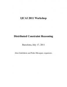
In Figure 15, the speed-up of GRASPER relative to CP(Graph) can be seen, showing that GRASPER presents better results than CP(Graph) for instances of the problem with order of at least 150. The speed-up was calculated as the quotient between the results of CP(Graph) and GRASPER. The chart clearly shows a large speed-up for graphs of order 150 and above. As no results were presented for the lysine chain of orders above 150 we were not able to analyse the speed-up for this chain but we believe that it would also present better results. CP(Graph) only produces slightly better results for the heme chain instances of order 100 and 150. However, this trend is clearly reversed for higher order instances: results for the glycosis chain outperform the ones obtained by CP(Graph) for every instance; results for the heme chain are better than the ones of CP(Graph) from order 200 above;

GRASPER: constraint reasoning with graphs results for graphs of order above 150 are all under 80 million cycles managing to decrease the expected time as compared to CP(Graph); finally, for the lysine chain, we could obtain results for instances of order above 150, for which CP(Graph) presents no results. Figure 15 GRASPER’s speed-up relative to CP(Graph) for the first-fail heuristic (see online version for colours)

89 The comparison between these frameworks seems to indicate that GRASPER’s ECLiPSe Constraint System implementation outperforms CP(Graph)’s Mozart implementation for larger problem instances, thus providing a more scalable framework. Table 3 presents the results obtained with our framework, implemented in CaSPER, for the naive (N), symmetric first-fail (SFF), greedy (G) and shortest-path (SP) heuristic. The results were obtained using the same Intel Core 2 Duo 2.16 GHz, 1.5 Gb of RAM, having been imposed a time limit of 10 minutes. The results for instance that were not solved within the time limit are set to ‘T.O.’. We present in Tables 4 and 5 a comparison between our framework, implemented in CaSPER and CP(Graph), implemented in Gecode for the symmetric first-fail and shortest-path heuristic, respectively. The results are presented in seconds and were obtained using an Intel(R) Celeron(R) 3 GHz, 750 Mb RAM (we could not manage to put CP(Graph) working on a Mac Os X 10.4 Intel Mac-Book Core 2 Duo 2.16 GHz, 1.5 Gb of RAM and so we had to rely on this Kubuntu Intel(R) Celeron(R) 3 GHz, 750 Mb RAM). Table 4

Table 3 Order 50

Metabolic pathways results Glyco N

SFF

G

SP

0.12

0.05

0.05

0.05

Order

Comparison between GRASPER and CP(Graph) with the symmetric first-fail heuristic Glyco GRASPER

CP(Graph)

50

0.07

0.02

0.19

0.10

100

1.75

0.16

0.29

0.22

100

150

7.89

0.93

0.49

0.51

150

1.44

0.89

200

25.30

1.91

0.88

0.91

200

3.63

T.O.

250

T.O.

4.13

1.15

1.11

250

8.29

T.O.

5.31

300

11.20

T.O.

300

T.O.

5.76

6.49

Lysine

Lysine GRASPER

CP(Graph)

50

0.07

0.08

1.09

100

0.23

1.50

0.48

T.O.

N

SFF

G

SP

50

0.06

0.06

0.06

0.06

100

0.28

0.19

8.84

150

136.00

0.41

11.80

1.91

150

200

T.O.

0.67

14.70

2.84

200

0.79

T.O.

250

T.O.

1.00

14.10

3.58

250

1.10

T.O.

300

T.O.

1.16

15.80

4.29

300

1.37

T.O. Heme

Heme GRASPER

CP(Graph)

N

SFF

G

SP

50

0.05

0.04

0.05

0.06

50

0.06

0.04

100

0.27

0.30

0.18

0.18

100

0.14

0.82

0.31

2.09

150

1.54

0.28

0.44

0.45

150

200

3.32

1.15

0.91

0.97

200

1.55

T.O.

250

2.20

1.50

1.26

1.38

250

1.90

T.O.

300

3.17

2.82

1.82

2.06

300

3.77

T.O.

90 Table 5

Order

R.D. Viegas and F.A. Azevedo Comparison between GRASPER and CP(Graph) with the shortest-path heuristic Glyco GRASPER

CP(Graph)

50

0.07

0.03

100

0.32

0.17

150

0.89

0.46

200

1.50

0.12

250

1.98

0.14

300

8.54

0.29 Lysine

GRASPER

CP(Graph)

50

0.08

0.07

100

1.46

0.22

150

2.61

0.23

200

4.07

0.21

250

5.46

0.44

300

7.82

0.45 Heme

GRASPER

CP(Graph)

50

0.09

0.03

100

0.31

0.06

150

0.64

0.07

200

1.36

0.08

250

2.11

0.10

300

3.50

0.10

Figure 16 GRASPER’s speed-up relative to CP(Graph) for the symmetric first-fail heuristic (see online version for colours)

In Figure 16 the speed-up of GRASPER relative to CP(Graph) can be seen, showing that GRASPER presents better results than CP(Graph) for instances of the problem with order of at least 100. The speed-up, as before, was calculated as the quotient between the results of CP(Graph) and GRASPER. Again no results were provided by

CP(Graph), in the time limit, for some of the higher instances of the problem. Although GRASPER achieves better results in its CaSPER implementation than in its ECLiPSe Constraint System implementation the speed-up obtained is not as high as the one we presented previously for the first-fail heuristic and GRASPER’s ECLiPSe Constraint System and CP(Graph)’s Mozart implementations. This may be due to the more efficient Gecode underlying framework and also the optimisations performed on CP(Graph). Opposingly to the results obtained for the symmetric first-fail heuristic, Table 5 presents CP(Graph) as having better results than GRASPER. In Figure 5, we present the speed-up of CP(Graph) relative to GRASPER with the speed-up calculated as the quotient between GRASPER’s and CP(Graph)’s results. As can be seen, CP(Graph) presents better results than GRASPER, achieving speed-ups higher than ten for the instances of order higher than 200 and above 20 for the instances of order 300. These last results seem to collide with the ones we obtained for the comparison between GRASPER’s ECLiPSe Constraint System and CP(Graph)’s Mozart implementation. We believe this is due to the optimisations performed on CP(Graph)’s Gecode implementation, where different graph data structures were tried and more powerful propagators were devised. In addition to having a more powerful underlying framework more advanced mechanisms were used in solving the metabolic pathways problem which, we believe, were essential in obtaining the results presented. One very important such mechanism is a cost-based filtering mechanism presented in Sellmann (2003). This cost-based filtering allows, at each search step, to determine the edges which must be removed since their inclusion would force the cost of the path to be higher than a given upper bound; and also to determine the edges which must be added since their removal would disallow the existence of the path, i.e., because those edges are bridges in the path. Since this mechanism can be done in polynomial time and is quite effective the results for the problem of the metabolic pathways decreased substantially when compared with the ones in CP(Graph) previous implementation. Another important aspect of CP(Graph)’s Gecode version is that it achieves more pruning than both its Mozart implementation and GRASPER, for the path constraint. At every step in the search phase, it determines the set of edges which must be removed from the path (because the edge jumps over a mandatory vertex, is not reachable from the start vertex or does not reach the final vertex) (Cambazard and Bourreau, 2004), the set of vertices that must be removed from the path (the vertex is isolated, is not reachable from the start vertex or does not reach the final vertex), the set of edges which must be added to the path (the edge is a bridge, or its end-vertices are mandatory and it is the only edge linking them) and finally the set of vertices that must be added to the path (its removal would disallow the existence of a path between the start and the final vertices) (Cambazard and Bourreau, 2004).

GRASPER: constraint reasoning with graphs The path constraint can, as we presented, be implemented upon the connected and quasipath constraints. The connected constraint in turn is based on the reachables constraint so, the more effective the reachables constraint is, the more efficient the connected constraint will be and, therefore, also the path constraint. As we admitted previously, we do not achieve full consistency for two filtering rules of the reachables constraint. In turn, CP(Graph) makes use of a fine tuned filtering mechanism based on Quesada et al. (2005) and Quesada (2006)’s work. Quesada (2006) introduces a reachability propagator for speeding up path constraint solvers, based on the concepts of transitive closure and dominators, and manages to achieve bounds-consistency. Figure 17 Grasper’s speed-up relative to CP(Graph) for the shortest-path heuristic (see online version for colours)

6

Remarks and future work

In this paper, we presented GRASPER, a framework for graph constraint problems, which defines graph variables as a composition of two set variables: a vertex-set and edge-set and was implemented upon Cardinal. We presented the core constraints and the high-level constraints provided by GRASPER, available at ECLiPSe Constraint System and CaSPER distributions. We then presented the filtering rules for the constraints implemented in our framework, first specifying the type of consistency we enforce in our constraints and then, for each constraint, the set of filtering rules it uses and their associated worst-case temporal complexity, stating the trigger and behaviour of each filtering rule. After presenting GRASPER we introduced the metabolic pathways problem, which is NP-hard, consisting in determining the shortest path between two given vertices, passing through a set of mandatory vertices and constrained not to pass simultaneously through given pairs of vertices. We presented a possible modeling, some search strategies to use and also the results obtained with our framework. The results obtained with our preliminary version of GRASPER

91 in ECLiPSe Constraint System proved to be more efficient and scalable than the preliminary version of CP(Graph) in Mozart. Comparing our preliminary version of GRASPER in CaSPER with CP(Graph)’s Gecode version allows one to conclude that CP(Graph)’s Gecode version is still better than GRASPER’s CaSPER version. We believe to have achieved GRASPER’s initial objectives. GRASPER is an intuitive, declarative and efficient graph constraint solver. However, there is still much effort to be invested in it, in order to be seen as a real alternative to CP(Graph). In order to improve the results for the metabolic pathways problem we intend to improve the heuristics used and we also intend to implement the cost-based filtering mechanism proposed in Sellmann (2003) since we believe this will have a major impact on the overall efficiency of solving the problem. Although heuristic optimisation is a concern, our main concern rests on the framework itself. The most complex constraints (e.g. connectedness and path) are dependent on the reachables constraint and so, the more efficient this constraint is, the more efficient these more complex constraints will be. As we admitted previously, we do not achieve full consistency for two of the filtering rules of the reachables constraint. CP(Graph) uses a very efficient filtering mechanism based on the work of Quesada (2006), which introduces a reachability propagator for speeding up path constraint solvers, based on the concepts of transitive closure and dominators, and manages to achieve boundsconsistency. So, we intend to study new algorithms for devising more efficient, declarative, set-based filtering rules for this vital constraint in order to boost our framework’s power and utility. We intend to test different implementations of graph variables. Both GRASPER implementations define graph variables as a composition of two set variables: a vertex-set and an edge-set. We intend to test other possible compositions like, for instance, a successor list format, which was used in CP(Graph)’s Gecode version. Additionally we intent to model some more graph-related real-life problems in order to express GRASPER’s usefulness in modelling these problems, and also some additional functionality, related or not with these specific problems, aiming at providing a robust, general and easy-to-use graph constraint framework. GRASPER is already available in version 5.10.103 of the ECLiPSe Constraint System distribution and will be soon available along with the CaSPER distribution, thus allowing the scientific community to test it thoroughly. We believe that GRASPER’s characteristics will attract the CP community and will allow it to more easily model graphrelated problems, at a higher level.

Acknowledgements Partially supported by PRACTIC-FCT-POSI/SRI/41926/ 2001 and SFRH/BD/41362/2007.

92


References Apt, K.R. (2003) Principles of Constraint Programming, Cambridge University Press. Attwood, T. and Parry-Smith, D. (1999) Introduction to Bioinformatics, Prentice Hall. Azevedo, F. (2007) ‘Cardinal: a finite sets constraint solver’, Constraints Journal, Vol. 12, No. 1, pp.93–129. Cambazard, H. and Bourreau, E. (2004) ‘Conception d’unecontrainte globale de chemin’, in Proceedings of the Dixièmes Journées Nationales sur la Résolution Pratique de Problèmes NPComplets (JNPC’04), pp.107–121. Chartrand, G. (1984) Introductory Graph Theory, Dover Publications. Chartrand, G. and Lesniak, L. (1996) Graphs and Digraphs, Chapman and Hall. Chartrand, G. and Oellermann, O. (1993) Applied and Algorithmic Graph Theory, McGraw-Hill. Cormen, T., Leiserson, C., Rivest, R. and Stein, C. (2001) Introduction to Algorithms, 2nd ed., MIT Press. Correia, M., Barahona, P. and Azevedo, F. (2005) ‘CaSPER: a programming environment for development and integration of constraint solvers’, in F. Azevedo, C. Gervet and E. Pontelli (Eds.): Proceedings of the First International Workshop on Constraint Programming Beyond Finite Integer Domains (BeyondFD’05), pp.59–73. Croes, D. (2005) ‘Recherche de chemins dans le réeseau métabolique et mesure de la distance métabolique entre enzymes’, PhD thesis, ULB, Belgium. Dechter, R. (2003) Constraint Processing, Morgan Kaufmann. Diestel, R. (2005) Graph Theory, Springer-Verlag. Dooms, G. (2006) ‘The CP(Graph) computation domain in constraint programming’, PhD thesis, Faculté des Sciences Appliquées, Université Catholique de Louvain. Dooms, G., Deville, Y. and Dupont, P. (2005) ‘CP(Graph): introducing a graph computation domain in constraint programming’, in Eleventh International Conference on Principles and Practice of Constraint Programming, Lecture Notes in Computer Science, No. 3709, pp.211–225, Springer-Verlag. Garey, M. and Johnson, D. (1979) Computers and Intractability: A Guide to the Theory of NP-Completeness, W.H. Freeman. Garey, M., Johnson, D. and Stockmeyer, L. (1974) ‘Some simplified NP-complete problems’, in STOC ‘74: Proceedings of the Sixth Annual ACM Symposium on Theory of Computing, pp.47–63, ACM. Gratzer, G. (1978) ‘General lattice theory’, Pure and Applied Sciences, Academic Press. Harary, F. (1969) Graph Theory, Addison-Wesley. Herrmann, J. (2006) Handbook of Production Scheduling, Springer-Verlag. Jensen, T. and Toft, B. (1995) Graph coloring problems, Wiley-Interscience. Jeong, H., Tombor, B., Albert, R., Oltvai, Z. and Barabási, A-L. (2000) ‘The large-scale organization of metabolic networks’, Nature, Vol. 406. Lala, P. (1996) Practical Digital Logic Design and Testing, Prentice Hall. Marriot, K. and Stuckey, P. (1998) Programming with Constraints: An Introduction, MIT Press.

Mathews, C. and van Holde, K. (1996) Biochemistry, 2nd ed., Benjamin Cummings. Musser, D. and Stepanov, A. (1988) ‘Generic programming’, in ISSAC, pp.13–25. Pinedo, M. (2006) ‘Planning and scheduling in manufacturing and services’, Operations Research and Financial Engineering, Springer-Verlag. Puget, J-F. (1992) ‘PECOS: a high level constraint programming language, in Proc. Spicis. Quesada, L. (2006) ‘Solving constrained graph problems using reachability constraints based on transitive closure and dominators, PhD thesis, Université Catholique de Louvain, Louvain-la-Neuve, Belgium. Quesada, L., van Roy, P. and Deville, Y. (2005) ‘Speeding up constrained path solvers with a reachability propagator’, in Colloquium on Implementation of Constraint and Logic Programming Systems (CICLOPS 2005), at the Eleventh International Conference on Principles and Practice of Constraint Programming (CP2005). Rossi, F., van Beek, P. and Walsh, T. (2006) ‘Handbook of constraint programming’, Foundations of Artificial Intelligence, Elsevier Science Inc. Russel, S. and Norvig, P. (2002) Artificial Intelligence: A Modern Approach, Prentice Hall. Schilling, C., Schuster, S., Palsson, B. and Heinrich, R. (1999) ‘Metabolic pathway analysis: basic concepts and scientific applications in the post-genomic era’, Biotechnology Programming, Vol. 15, No. 3. Sellmann, M. (2003) ‘Cost-based filtering for shorter path constraints’, in Proceedings of the Ninth International Conference on Principles and Practice of Constraint Programming (CP), Lecture Notes in Computer Science, Vol. 2,833, pp.694–708, Springer-Verlag. Schuster, S., von Kamp, A. and Pachkov, M. (2008) ‘Understanding the roadmap of metabolism by pathway analysis’, Methods in Molecular Biology, Chapter Biomedical and Life Sciences, Vol. 358, pp.199–226, Humana Press. Tsang, E. (1983) Foundations of Constraint Programming, Academic Press. van Helden, J., Wernisch, L., Gilbert, D. and Wodak, S. (2002) Graph-Based Analysis of Metabolic Networks, pp.245–274, Springer-Verlag. Waterman, M. (1995) Introduction to Computational Biology, Chapman and Hall/CRC. Xu, J. (2003) ‘Theory and application of graphs’, Network Theory and Applications, Vol. 10, Kluwer Academic Publishers.