Abstract: In this paper we present a simple modification of some cascade-correlation type constructive neural network algorithms. The key idea of the ...
Constructive Neural Networks - Automated Allocation of Hidden Units into Hidden Layers JANI LAHNAJÄRVI, MIKKO LEHTOKANGAS, AND JUKKA SAARINEN Digital and Computer Systems Laboratory Tampere University of Technology P.O.BOX 553, FIN-33101 Tampere FINLAND
Abstract: In this paper we present a simple modification of some cascade-correlation type constructive neural network algorithms. The key idea of the modification is to use two types of candidate units instead of only one type of candidates used in the standard versions. The best candidate unit, which is installed in the active network, either becomes part of the current deepest hidden layer or adds a new hidden layer to the network. The modification enables the algorithms to create more varying and shallower network topologies than those created with the standard versions of the algorithms. The investigated algorithms were Cascade-Correlation, Modified CascadeCorrelation, Cascade, and Fixed Cascade Error. The simulations showed that the new versions of the algorithms produce approximately half as deep networks as the standard versions. The overall computational load of the new versions stayed at the same level when compared to the old versions of the algorithms. The main reasons were, on the other hand, the slightly increased number of the hidden units and, on the other hand, the decreased number of the network connections in the sparse topologies created by the new versions of the algorithms. Furthermore, the generalization performance was noted to improve nearly in all the cases. Key-Words: Constructive neural networks, connection strategies of hidden units, regularization, generalization, cascade-correlation, classification, regression.
1 Introduction In its complete form, neural network training consists of parametric and structural learning, i.e. learning both weight values and an appropriate topology of neurons and connections. Current connectionist methods to solve this task fall into two broad categories. Constructive algorithms use a minimal initial network and add neurons and connections as needed. Pruning algorithms, on the other hand, start with a large initial network and prune off unimportant components. Although these algorithms address the complete problem of model selection, they do so in a highly constrained manner. Generally, constructive and pruning methods limit the available architectures in some way. Such structural hill climbing methods are susceptible to becoming trapped at structural local optima, which places the burden of model selection mostly on the learning of suitable parametric values rather than distributing the burden evenly. As a consequence, these algorithms tend to force a task into an assumed architectural class rather than fitting an appropriate architecture to the task [2]. The standard cascade-correlation algorithm [4] is a fine example of such constrained constructive algo-
rithms. It always forms the networks by training new hidden units one by one and adding each of them on a separate hidden layer in the active network. Thus, addition of each hidden unit creates a new layer in the network, which means that the resulting networks may be much deeper than necessary for solving the problem efficiently [1]. Moreover, if we have a large pool of neural networks created by cascade-correlation, we notice that the networks having equal number of hidden units are always exactly similar in their topology. This is a clear indication of the weakness of the cascade-correlation algorithm in forcing a neural network architecture to the problem at hand. This paper presents a slight modification of some cascade-correlation type constructive neural network algorithms. The modification enables the networks to learn problems by varying the number of the hidden units in the hidden layers thus making it possible to create more complex network topologies than with the standard versions of the algorithms. The resulting enhanced algorithms still preserve their ability to build deep nets when needed. Moreover, the deepness of the networks can easily be adjusted by a userdefined parameter.
2 Investigated Algorithms We studied four different constructive neural network algorithms. The investigated algorithms were Cascade-Correlation (CC) [4], Modified Cascade-Correlation (MCC) with objective function S2 presented in [6], Cascade (CAS) [14], and Fixed Cascade Error (FCE) [7]. We used two different versions of all these algorithms in our simulations. The first versions (i.e. fixed hidden layer size versions) had fully cascaded architecture. This means that the hidden units were added each on a separate hidden layer just like in standard cascade-correlation. The second versions (i.e. varying hidden layer size versions) had different architecture. The hidden units were added either on a new deeper hidden layer or to the current deepest layer, which enables the algorithm to create shallower networks. In both of the versions we applied regularization [3] in the candidate hidden unit and output unit training. The performance of the algorithms was then assessed based on numerical simulations both with classification and regression problems.
C C, j =
∑ ( Vj, l – Vj ) ( El – E ) –ν ∑ wij, j 2
l
The cascade-correlation [4] learning begins with a network having no hidden units at all and it automatically adds new hidden units until a satisfactory solution is achieved. Once a new hidden unit has been added to the network, its input weights are frozen. This unit then becomes a permanent feature detector in the network, and it produces outputs for possibly additional hidden units creating more complex feature detectors. The cascade-correlation architecture has been reported to have several advantages over conventional non-constructive backpropagation algorithms [4]. The fixed hidden layer size versions of the investigated algorithms can be presented in the following way. First, q (q = 8 in our study) candidate units are created by initializing their weights with uniformly distributed random numbers of the range [-0.5, +0.5] (the same range was used also in the second versions of the algorithms). Next, all the q candidates are trained to their final values with RPROP algorithm [15] by employing the regularized versions [8], [9] of the standard objective functions in the update rule. The differences between the algorithms, which are mainly in the objective function, are clarified next. For the first benchmark algorithm, the standard Cascade-Correlation algorithm designed by Fahlman and Lebiere [4], the maximizable objective function is given by
(1)
where Vj,l is the output of the jth candidate unit for the lth training pattern, Vj the mean of the jth candidate unit outputs, El is the network output error (one output unit in all our simulations) for the lth training pattern, E is the mean of the network output errors, ν is the regularization parameter, and wij is the network weight that connects the input unit (or pre-existing hidden unit) i to the candidate unit j. In Modified Cascade-Correlation algorithm [6] the candidate hidden units are trained by maximizing the regularized version of S2 [6], which is given by
∑ Vj, l El –ν ∑ wij, j 2
S 2,j =
l
= 1, …, q.
(2)
i
In Cascade algorithm [14] we use a minimizable squared error cost function, which is defined as C E, j =
∑ ( tl – oj, l ) l
2.1 Versions with Fixed Hidden Layer Size
= 1, …, q,
i
2
+ ν ∑ w ij, j = 1, …, q, 2
(3)
i
where oj,l is the actual network output for lth training pattern with the jth candidate unit in the network and tl is the target output of the network for the lth training pattern. This cost function also means that we have to update the output weight of the candidate unit after each epoch during the candidate unit training, which leads to higher computational complexity than in the other algorithms. Finally, in the Fixed Cascade Error algorithm [7] we use a maximizable cost function [8] defined by C FE, j =
∑ ( El – E )Vj, l –ν ∑ wij, j 2
l
= 1, …, q.
(4)
i
After all the q candidate hidden units have been trained and the values of the objective function (related to the particular algorithm) have been recorded, the optimum (max or min) value of the regularized cost function among all the candidates is searched. The corresponding candidate unit j is selected to be the most promisingly trained hidden unit which is then installed in the active network and all the other candidate hidden units are deleted. After installing the new hidden unit into the network, the network output unit is trained by the regularized pseudo-inverse method of linear regression. Because of the activation function of the output unit being a linear one, we are able to solve the output unit weights analytically. The regularized cost function for the output unit is a squared error function [5], [11]
C out =
∑ El + µ ∑ vi 2
l
2
T
T
= ee + µvv ,
(5)
i
where µ is the regularization parameter, e1×n is the output error vector, and v1×(p+h+1) is the weight vector (including bias) of the output unit. Here the number of the training patterns is n, the number of network inputs is p, and the number of the hidden units installed in the network is h. Now, the optimum value for v which minimizes the objective function can be found by setting the gradient of the objective function to zero. That equation solves easily as [9] T
T
–1
T
v = ( RR + U ) Rt .
(6)
where R(p+h+1)×n is the input matrix of the output unit and U(p+h+1)×(p+h+1) is a diagonal regularization matrix in which all the diagonal elements are µ’s, and t1×n is the target output vector of the network. This whole cycle of training the candidate units, selecting and installing the best one of them, and training the output unit is repeated when a new hidden unit is to be added to the network.
2.2 Versions with Varying Hidden Layer Size A simple modification of all the investigated algorithms was studied in order to decrease the depth of the resulting networks and to create more varying network topologies. We simply split the pool of candidate hidden units into two groups. One group, the q1 descendant units (q1 = 4 in our study), operates just as all the candidates described in the previous section. They all receive inputs from all network inputs and pre-existing hidden unit outputs thus adding one hidden layer into the active network. The other group, the q2 sibling units (q2 = 4 in our study),
receives inputs only from earlier layers of the network but not from those units that are currently in the deepest hidden layer of the net. When sibling units are added to the active network, they become part of the current deepest hidden layer and they do not begin a new deeper layer in the network. During candidate unit training, the sibling and descendant units compete with one another. The one with the best score in the objective function is chosen for installation in the active network. Thus, the network will only be deepened in cases where a descendant unit gives us the best value. During the study, we noticed that the descendant units have normally a clear advantage over the sibling units. This is not surprising since the descendant units share the same inputs as the sibling units plus one or more inputs from the deepest hidden layer. However, in some cases the additional inputs may be harmful and they can make the descendant units converge slower. Anyway, these cases were noticed to be rather rare which means that the networks grew almost as deep as in the fixed hidden layer size versions described in the previous section. In order to create shallower networks, we decided to penalize the descendant units. This was done by multiplying the value of the objective function (given in Equations 1 to 4 for different algorithms) with a penalty factor λ. This λ value was set to 1 for the sibling units and to a smaller value for the descendant units with the CC, MCC, and FCE algorithms (since in those algorithms we are maximizing the cost function value). For CAS algorithm, this λ value for the descendant units had to be set to a larger value than (or equal to) 1, since in that algorithm we aim to minimize the cost function value. The exact parameter values for all the algorithms and simulation problems are given in section 3.
Output
Hidden
6
Input
Figure 1. Examples of different network architectures with six hidden units in all of them. On the left normal cascaded architecture with one hidden unit in each of the six hidden layers. On the middle and right sibling/descendant network architectures with six hidden units in two hidden layers in both cases. Each hidden unit has input connections from every unit in the preceding layers.
This modification of the algorithms by splitting the candidate pool into two groups leads to large differences in the network architecture. If we have some particular number of hidden units in the network, the fixed hidden layer size versions of the algorithms lead every time to the same network in its topology. In the sibling/descendant versions, networks with same number of hidden units can be considerably different architecturally. Some examples of such resulting architectures are given in Figure 1. The use of separate sibling and descendant units (in CC algorithm) was first published by Baluja and Fahlman [1]. The differences to our research are that they studied only the cascade-correlation algorithm and that they did not use regularization at all while training the networks. We, on the other hand, applied this sibling/descendant approach to four different constructive algorithms and used regularization both in the hidden and output unit training phases as described in section 2.1. Regularization was applied in order to enhance generalization performance [3], [5], which Baluja and Fahlman reported not to have been improved in their simulations with the sibling/ descendant modification.
3 Simulations and Results The algorithms were tested in extensive simulations with four classification and four regression problems. The classification problems were Chess [10], Spiral [4], 10-bit Parity [4], and Cancer diagnosis problem [13]. The regression problems were Henon map [10], Laser time series [16], Additive function approximation [6], and Mackey-Glass chaotic time series [12]. The Cancer and Laser problems are based on realworld data while the others are artificially generated. All the simulations were repeated twenty times due to the random initialization of the network weights. The regularization parameter ν was set to 0.01 for the both versions of the CC, MCC, and FCE algorithms in all the problems. For the fixed hidden layer size version of the CAS algorithm we used a parameter ν value of 10-5 in Chess, Cancer, Laser, and Additive problems while in Spiral, Parity, Henon, and Mackey problems we utilized a parameter ν value of 5×10⁻⁶. For the varying hidden layer size version of the CAS algorithm we used a parameter ν value of 5×10⁻⁶ in all the problems. The regularization parameter µ was set to 0.0001 for both versions of all the algorithms. The penalty factor λ was defined according to the following discussion. First, the deepness of the net-
works can easily be adjusted by the penalty factor λ: the more we penalize descendant units, the shallower the networks grow. Second, we must not, however, favour the sibling units too much since in some of the problems we studied it is clearly favourable to have many hidden layers in the network solution. (In the beginning of this study, we examined one-hiddenlayer versions of the algorithms, and they encountered huge problems especially in Spiral and Mackey problems. This proved us that we should have at least some descendant units in the final network.) After some experiments with different λ values, the penalty factor λ of the descendant units was set to 0.85 for the CC, MCC, and FCE algorithms in Chess, Spiral, and Parity problems while in Cancer, Henon, Laser, Additive, and Mackey problems we used a value of 0.75 (denoting more penalty). For the CAS algorithm we used the following λ values: λ = 1.00 for Spiral, Cancer, and Mackey; λ = 1.01 for Chess and Laser; λ = 1.015 for Additive; λ = 1.02 for Parity and λ = 1.03 for Henon problem. This means that we do not penalize the descendant units at all in Spiral, Cancer, and Mackey problems with the CAS algorithm. As can be guessed from the parameter values, the CC, MCC, and FCE algorithms were not very sensitive to the selection of the penalty factor λ, while for the CAS algorithm selecting that factor had to be done more carefully. Since all the candidate hidden units had sigmoidal activation function (hyperbolic tangent), they were trained with RPROP algorithm [15]. The hidden unit training was continued until the changes in the objective function value were sufficiently small or the maximum number of the epochs was reached. The output units were trained by the pseudo-inverse method of linear regression as discussed in section 2.1. The network training was stopped when the network output error fell below the target error value or the maximum number of the hidden units was reached. The error values that we used for computing the simulation results were classification error (CERR) for the classification problems and normalized mean square error (NMSE) for the regression problems [8]. The final results are shown in Table 1. In each case, the averaged best result of the testing data and the average numbers of hidden units, hidden layers, and MFLOPS (millions of floating point operations) are shown. The upper row in all the cases shows the results obtained with the varying hidden layer size version of the particular algorithm while the lower row gives the results with the fixed hidden layer size
version of the algorithm. In Chess and Spiral problems the results are shown according to the training data since there were no testing data available in those problems. For the readers’ convenience, the best result of each item among both the versions of the algorithms is shown in ‘bold’ for each problem. In case of many equally best results in a single problem, all the best results in that particular problem are given in ‘bold’. The results in Table 1 state that the new sibling/ descendant approach diminishes radically the number of the hidden layers in the resulting networks. The changes in the numbers of the hidden layers are in the range of -74% to -30% showing that the networks created by the standard algorithms are on average twice as deep as those created by the new algorithms. When we consider the number of the hidden units, we note the changes being in the range of -28% to +29%, respectively. Though that range is rather wide, the variations in the numbers of the hidden units are mainly very small (normally in favour of the old versions). Only a few cases are noticed where the changes in the number of the hidden units are larger than 10%. The variations in the generalization performance are in nearly all the cases in favour of the new versions of the algorithms. However, the extreme range in that change is from -30% to +35%, which shows that without some single inferior results especially in Parity problem there would be a perfect record for the sibling/descendant versions. The enhancements in favour of the new versions can especially be seen in Additive function problem, where all the algorithms give considerably better results with their sibling/ descendant versions. Moreover, when we study the respective change in the number of MFLOPS we can observe that range to be from -38% to +29%. The main reason for these variations is the varying number of the hidden units in the final networks. Moreover, even if the new approach uses two different types of candidates in the hidden unit training, it actually decreases slightly the computational complexity of the algorithms. That is due to the fact that the reduced number of the hidden layers diminishes the number of the free parameters in the networks and, likewise, the number of needed operations in the network training. This means that the more there are hidden units in the networks, the more favourable the situation is for the new versions of the algorithms. If the networks have the same number of hidden units, the new versions usually need a couple of percent less MFLOPS than the old versions.
Finally, when we compare the results of the new version of each algorithm to those of its old version, we notice that the new approach works best with the FCE algorithm. The results with the new sibling/ descendant versions show that the FCE algorithm is computationally the easiest one and that it provides us the best error values and smallest networks on average. The MCC algorithm is found to tie with the FCE algorithm in finding the shallowest networks on average. Moreover, the CAS algorithm is yet again noted to be computationally the most demanding algorithm.
4 Conclusions We presented a modification for some cascade-correlation type constructive neural network algorithms. The key idea of the modification is to split the pool of candidate hidden units into two groups. The candidate, which is installed in the active network, either becomes part of the current deepest hidden layer (the sibling units) or adds a new hidden layer to the network (the descendant units). This modification enables the algorithms to create more varying and shallower network topologies than those created with the standard versions of the same algorithms. The simulations showed that the new versions of the algorithms produce clearly (approximately 50%) shallower networks than the old versions. The overall computational load of the new versions stayed at the same level when compared to the old versions. This was partly due to the slightly increased number of the hidden units and partly because of the reduced number of the network connections in the new algorithms. Furthermore, the generalization performance was noticed to improve in almost all the cases.
References: [1] S. Baluja and S. E. Fahlman, “Reducing Network Depth in the Cascade-Correlation Learning Architecture”, Technical Report CMU-CS-94-209, School of Computer Science, Carnegie Mellon University, Pittsburgh, PA, 1994. [2] P. J. Angeline, G. M. Saunders, and J. B. Pollack, “An Evolutionary Algorithm that Constructs Recurrent Neural Networks”, IEEE Transactions on Neural Networks, Vol. 5, No. 1, Jan. 1994, pp. 54-65. [3] C. M. Bishop, “Regularization and Complexity Control in Feed-Forward Networks”, Technical Report: NCRG/95/022, Neural Computing Research Group, Dept. of Computer Science and Applied Mathematics, Aston University, Birmingham, UK, 1995.
[4] S. E. Fahlman and C. Lebiere, “The Cascade-Correlation Learning Architecture”, Technical Report CMUCS-90-100, School of Computer Science, Carnegie Mellon University, Pittsburgh, PA, 1990. [5] S. Haykin, Neural Networks: A Comprehensive Foundation, MacMillan College Publishing Company, New York, 1994. [6] T.-Y. Kwok and D.-Y. Yeung, “Objective Functions for Training New Hidden Units in Constructive Neural Networks”, IEEE Transactions on Neural Networks, Vol. 8, No. 5, Sep. 1997, pp. 1131-1148. [7] J. Lahnajärvi, M. Lehtokangas, and J. Saarinen, “Fixed Cascade Error - A Novel Constructive Neural Network for Structure Learning”, Proceedings of the Artificial Neural Networks in Engineering Conference, ANNIE’99, St. Louis, Missouri, USA, Nov. 710, 1999, pp. 25-30. [8] J. Lahnajärvi, M. Lehtokangas, and J. Saarinen, “Constructive Neural Networks with Regularization Approach in the Hidden Unit Training”, International NAISO Congress on Information Science Innovations, ISI’2001, Dubai, UAE, Mar. 17-21, 2001, accepted paper, 7 pages. [9] J. Lahnajärvi, M. Lehtokangas, and J. Saarinen, “Constructive Neural Networks with Regularization”, 2001 WSES International Conference on Neural Networks and Applications, NNA’01, Puerto De La Cruz, Spain, Feb. 11-15, 2001, submitted (invited) paper, 6 pages.
[10] M. Lehtokangas, J. Saarinen, P. Huuhtanen, and K. Kaski, “Initializing Weights of a Multilayer Perceptron Network by Using the Orthogonal Least Squares Algorithm”, Neural Computation, Vol. 7, No. 5, 1995, pp. 982-999. [11] M. Lehtokangas, “Pattern Recognition with Novel Support Vector Machine Learning Method”, Proceedings of the X European Signal Processing Conference, EUSIPCO-2000, Tampere, Finland, Sep. 5-8, 2000, Vol. 2, pp. 733-736. [12] Oregon Graduate Institute of Science and Technology, Data Distribution WWW site (http:// www.ece.ogi.edu/~ericwan/data.html). [13] L. Prechelt, “PROBEN1 - A Set of Neural Network Benchmark Problems and Benchmarking Rules”, Technical Report 21/94, Fakultät für Informatik, Universität Karlsruhe, D-76128 Karlsruhe, Germany, Sep. 1994. [14] L. Prechelt, “Investigation of the CasCor Family of Learning Algorithms”, Neural Networks, Vol. 10, No. 5, 1997, pp. 885-896. [15] M. Riedmiller and H. Braun, “A Direct Adaptive Method for Faster Backpropagation Learning: The RPROP Algorithm”, Proceedings of the IEEE International Conference on Neural Networks, San Francisco, CA, Mar. 28 - Apr. 1, 1993, pp. 586-591. [16] The Santa Fe Time Series Competition Data WWW site (http://www.stern.nyu.edu/~aweigend/TimeSeries/SantaFe.html).
Table 1. The results of the algorithms with all the simulation problems. The values are the error value (ERR), the number of hidden units (HU), hidden layers (HL), and MFLOPS (MF) spent during the training phase, respectively. Problems marked with an asterisk (*) give CERR and the others give NMSE as their error values. In each case, the upper values are for the new versions of varying hidden layer size (VS) and the lower values are for the old versions of fixed hidden layer size (FS). The results are average values of twenty runs. Algorithm
CC
MCC
CAS
FCE
Problem
ERR
HU
HL
MF
ERR
HU
HL
MF
ERR
HU
HL
MF
ERR
HU
HL
MF
Chess* VS FS
0 0
3.30 3.45
2.00 3.45
0.84 0.93
0 0
3.35 3.25
1.90 3.25
0.76 0.80
0 0
3.15 3.25
2.10 3.25
1.70 1.84
0 0
3.10 3.05
1.95 3.05
0.65 0.69
Spiral* VS FS
0 0
19.15 11.35 136 19.15 19.15 139
0 0
19.20 11.10 129 19.10 19.10 132
0 0
19.05 12.05 280 17.35 17.35 249
0 0
18.10 10.65 112 18.60 18.60 121
Parity* VS 0.0168 FS 0.0144
6.75 5.80
3.40 5.80
165 144
0.0168 0.0124
7.05 6.75
3.75 6.75
168 167
0.0166 0.0221
8.60 8.40
3.70 8.40
422 419
0.0139 0.0148
7.40 7.30
4.15 7.30
170 174
Cancer* VS 0.0225 FS 0.0232
2.50 2.45
1.10 2.45
28.0 27.6
0.0231 0.0231
2.40 3.35
1.05 3.35
25.0 40.2
0.0222 0.0215
2.55 2.70
1.50 2.70
60.7 67.1
0.0209 0.0221
2.60 2.50
1.25 2.50
26.4 26.4
8.45 8.05
3.90 8.05
18.1 18.0
0.0261 0.0279
8.85 8.40
3.90 8.40
17.9 17.9
0.0375 0.0372
8.95 8.40
3.80 8.40
47.5 47.0
0.0268 0.0281
8.45 8.20
3.55 8.20
15.8 16.5
Henon
VS 0.0276 FS 0.0295
Laser
VS 0.0254 16.75 5.55 778 FS 0.0256 15.85 15.85 765
0.0233 16.65 5.45 751 0.0248 15.45 15.45 712
0.0245 17.20 6.70 1840 0.0221 16.00 5.80 692 0.0271 15.60 15.60 1610 0.0253 15.65 15.65 708
Additive VS 0.0239 17.60 6.05 205 FS 0.0317 17.50 17.50 219
0.0223 16.65 6.15 180 0.0320 17.55 17.55 210
0.0311 18.95 4.45 507 0.0443 17.20 17.20 482
0.0262 17.45 6.50 185 0.0362 16.55 16.55 188
Mackey- VS 0.3205 Glass FS 0.3270
0.3200 0.3264
0.3302 0.3301
0.3186 0.3237
8.00 6.20
2.80 6.20
97.0 74.9
8.25 6.85
2.75 6.85
96.5 81.6
7.60 7.95
4.85 7.95
183 208
7.25 6.40
2.65 6.40
75.9 68.8