Modeling Semi-Automated Forces with Neural Networks: Performance Improvement through a Modular Approach Amy E. Henninger Avelino J. Gonzalez Michael Georgipoulos Ronald F. DeMara School of Electrical Engineering and Computer Science University of Central Florida Orlando, FL 32816-2450
[email protected] Keywords: Neural networks, Human behavior representation
ABSTRACT:. A recent report by the National Research Council (NRC) declares neural networks “hold the most promise for providing powerful learning models”. While some researchers have experimented with using neural networks to model battlefield behavior for Computer Generated Forces (CGF) systems used in distributed simulations, the NRC report indicates that further research is needed to develop a hybrid system that will integrate the newer neural network technology into the current rule-based paradigms. This paper supports this solicitation by examining the use of a context structure to modularly organize the application of neural networks to a low-level Semi-Automated Forces (SAF) reactive task. Specifically, it reports on the development of a neural network movement model and illustrates how its performance is improved through the use of the modular context paradigm. Further, this paper introduces the theory behind the neural networks’ architecture and training algorithms as well as the specifics of how the networks were developed for this investigation. Lastly, it illustrates how the networks were integrated with SAF software, defines the networks’ performance measures, presents the results of the scenarios considered in this investigation, and offers directions for future work.
1. Introduction The combination of computer simulation and networking technologies has provided military forces with an effective means of training through the use of Distributed Interactive Simulation (DIS). DIS is an architecture for building large-scale simulation models from a set of independent simulator nodes that represent entities in the simulation [1]. These simulator nodes individually simulate the activities of one or more entities in the simulation and report their attributes and actions of interest to other simulator nodes via the network. DIS nodes simulating combat vehicles, such as M1 Abrams tanks, are crewed by soldiers being trained. The trainees operate the controls of the simulators as they would in the actual vehicles, and the simulators implement actions in the simulated battlefield. Since, in a synthetic battlefield, the trainees need opposing forces against which to train, a type of DIS node known as a Computer Generated Force (CGF) system was developed. CGFs are computer-controlled behavioral models of combatants used to serve as opponents against whom
trainees can fight or as friendly forces with which the trainees can fight. At a minimum, the behavior generated should be feasible and doctrinally correct. For example, behaviors should be able to emulate the use of formations in orders, identify and occupy a variety of tactical positions (e.g., fighting positions, hull down positions, turret down positions, etc), and plan reasonable routes. Researchers in [2], [3], and [4] have experimented with using neural networks to model battlefield behavior for CGF systems used in military simulations. This technology has been identified as one that “holds the most promise for providing powerful learning models” in a recent National Research Council Report [5]. Also asserted in this report, however, is the need for further research to develop hybrid systems that will integrate the newer neural network technology into the current rulebased paradigms. This investigation considers one such approach by using a framework based on modular decomposition to develop and apply the neural networks generating SAF behavior. Specifically, this research examines the performance improvements made to a
neural network based near-term movement model by adopting a modular approach.
3.
Neural Networks
A variety of researchers have worked in modeling human driving skills such as acceleration, steering, and vehicle following with neural networks [15], [16], [17], and [18]. A neural network is a collection of simple processors or nodes interconnected with each other that learn from examples and store the acquired knowledge in their interconnections, referred to as weights. Neural networks can solve a variety of problems related to non-linear regression and discriminant analysis, data reduction, and non-linear dynamic systems. One of the practical characteristics of neural networks is that they lend themselves to parallel-distributed processing using simple processing units rather than a complex CPU. This makes their execution very fast.
2. Modular Decomposition The use of a modular approach to a modeling task can be beneficial in a variety of ways. For example, it can be used for the purposes of improving performance. In other words, although the task could be solved with a monolithic set, better performance is achieved when it is broken down into a number of expert modules. Once the task is decomposed it is possible to switch to the most appropriate module, depending on the current circumstances or context. Switching has been discussed in the control literature [6][7], as well as the literature on behavior-based robotics [8].
The multi-layer feed-forward network is one of the more typical network designs used in neural network applications. The example in Figure 1 is a 3-layer feed-
In addition to performance improvement, other motivations for adopting a modular approach to a problem include a reduction in model complexity and construction of the overall system such that it is easier to understand, modify, and extend. Thus the “divide and conquer” principle is used to reduce the complexity of a single net system. This enables the use of different neural net architectures or algorithms to be applied to individual sub-problems, making it possible to exploit specialist capabilities. Moreover, where appropriate, some of these components could make use of non-neural computing techniques. This justification has been noted [9][10] and is common to engineering design in general. Another motivation for adopting a modular approach is the reduction of network training times [11]. Finally, in welldefined domains, the use of a priori knowledge can be used to suggest an appropriate decomposition of a task. This approach complements the knowledge acquisition efforts and knowledge representation paradigms used in current SAF systems [12] and can be easily extended to the acquisition of knowledge and tactics for SAF systems [13].
x1
01 w 31
x2
02
w 21
w 11 w 12
11 w 11 w 21
w 22
w 13
12
21
y1
22
y2
w 12 w 22
x3
03
w 23
w 32
w 13 w 23
w 14 x4
w 24
w 33
13
w 34
04
Where • x1, x2, x3 and x4 are inputs (k = 1 to 4) • y1 and y2 are outputs (i = 1 to 2) • there are three hidden nodes (j = 1 to 3) • there are three layers (L = 0,1,2) • node “12” is node 2 in layer 1 • weight “12” connects node 1 from layer L+1 to node 2 of layer L
The decomposition of a problem into modular components may be accomplished automatically or explicitly. When the decomposition of the task into modules is determined explicitly, this usually relies on a strong understanding of the problem. The division into sub-tasks is known prior to training [14], and improved learning and performance can result. An alternative approach is one in which the task is automatically decomposed according to the blind application of a data partitioning technique. Automatic decomposition is typically applied with the intent of performance improvement, whereas explicit decomposition could have the aim of either improving performance or accomplishing tasks that might not be accomplished as easily or as naturally with a monolithic net.
Figure 1. 4-3-2 Feed-Forward Architecture forward network with four nodes in the first layer representing each dimension of the input vector, two nodes in the last layer representing each dimension of the output vector, and a hidden layer consisting of three nodes. This network attempts to develop a matching function between the input and output vectors by using some training algorithm. One of the more popular training algorithms is a method known as backpropagation. This method is based on finding the outputs
2
η is a user defined parameter. By applying the chain rule of derivation (see [19] for complete derivation), equations 5.1 and 5.2 reduce to: ∆wij( 2 ) = ηδ i( 2) ( p) y (j1) ( p) i = 1,2 j = 1,2,3 (5.1)
at the last layer of the network, calculating the errors between the actual and the predicted outputs, and then adjusting the network weights to minimize the error. Weight changes are implemented in a backward fashion starting from the weights converging to the output layer and proceeding backwards to the weights that converge to the hidden layer closest to the output layer. These computations are repeated such that the error is propagated back until the weights converging to the hidden layer closest to the input layer are reached.
where δ i( 2) ( p) = g ′(neti( 2) ( p))[d i( 2) ( p) − yi( 2 ) ( p)] ∆w(jk1) = ηδ (j1) ( p) x k ( p)
where δ (j1) ( p) = g ′(net (j1) ( p ))
In short, back-propagation involves a two step process. The first step, the forward pass, propagates the effects of the inputs forward through the network to reach the output layer. This step is governed by three forms of equations. First, in equation 1.1, the total weighted input to the jth node for pattern p is given by: net (j1) ( p) =
K =4
∑x
( 0) (1) k ( p ) w jk
for j = 1 to 3
1 1+ e
J =3
∑y
(1) ( 2) j ( p ) wij
for i = 1 to 2
(1.1)
∆w(jk1) = η ( y j ( p))(1 − y j ( p))
∑[ d
(2) i ( p)
− yi( 2) ( p)]2
(1.2)
(6.2)
4. Methodology This study used ModSAF, a CGF system for training and research, to focus on the near-term movement behavior of a SAF. The near-term movement behavior was selected because it is computationally challenging and highly observable [20], [21], [5]. It also provides a direct correspondence to ESPDUs resulting from errors in entity position. This proves useful in finding a way to measure the performance of this study as explained in the next section (section 5). However, since moving in the battlefield is a highly complex behavior depending on many factors, the problem was scoped to specifically consider how a single entity (i.e., a ModSAF M1A2) performs a “Road March”. This is accomplished by estimating the changes in an M1A2 entity’s speed and orientation given its previous state and the previous state of the simulated world
(3)
i =1
∂ ) ∂w(jk)
i
Each of these weight adjustments directs the network towards a solution to the input/output mapping. That is, these weights are training the network to produce a certain output given a set of inputs. This is one of the fundamental benefits of the neural network approach. With the proper training and representation, the network will self-organize to arrive at a mapping of how the responses are formed and there is no need to acquire and represent an expert’s knowledge in terms of rule sets.
Once the error is computed, the weights are adjusted such that Ep is minimized. This occurs in the second pass, the backward pass, by computing the negative gradient of the error function and taking the partial derivatives of this function with respect to the weights (equations 5.1 and 5.2). This allows errors at the output layer to be propagated backward toward the input layer in proportion to the change in activity at the previous layer. ∂E (4.1) ∆wij( 2 ) = −η ( ( 2 ) ) ∂wij ∆w(jk) = −η (
∑[( y ( p)) ⋅
(2.1)
where g () is shown as the sigmoid function. Lastly, the error function associated with the pth input/desired output (dI(p)) pair, is given by: I =2
I =2
(1 − yi ( p))(d i ( p ) − yi ( p ))wij( 2) ] ⋅ xk ( p)
j =1
1 2
( 2 ) ( 2) ij δ i ( p )
i =1
and the output of the ith node for pattern p, yI(p), is given by: 1 (2.2) yi( 2) ( p ) = g (neti( 2) ( p)) = −neti ( p ) 1+ e
E p ( w) =
∑w
( y (j1) ( p))
where g () is the frequently used sigmoid function. The net input to the ith node for pattern p is similar to equation (1.1) and is given by: neti( 2 ) =
(5.2)
For the example in Figure 2, these equations reduce to: ∆wij( 2 ) = η ( yi ( p))(1 − yi ( p))(di ( p) − yi ( p)) ⋅ (6.1)
Next, the output of the jth node, y (j1) ( p) , is given by: −net j ( p )
I =2 i =1
k =1
y (j1) ( p) = g (net (j1) ( p)) =
j = 1,2,3 k = 1,2,3,4
For this application, a feed-forward architecture with back-propagation training was used in each of experimental systems. In the first system, Model 1, two
(4.2)
3
networks were considered. One of these networks predicts the change in an entity’s speed and the second network predicts the change in the entity’s heading. In the second system, Model 2, four networks were considered. Of these four neural networks, two predict the change in the entity’s speed and the other two predict the change in the entity’s orientation. Each of these pairs of networks can be further distinguished by whether the M1A2 entity is traveling a straight segment of the road or is entering a turn. The rule used to distinguish between these segment types was acquired from the code used to generate the SAF’s behavior and is based on the straightline distance to the current waypoint. This decomposition category is referred to as a “context” and the change from one context to another context is referred to as a “context transition” [22]. In this problem, for example, there are two contexts: straight and turning. Also, there is a rule defining when to shift between contexts:
S t = S t −1 + ∆S t where ∆S t = f(Rat −1 ,Rbt −1 ,Rct −1 ,Rpt −1 , Rs t −1 ,HRabt −1 ,HRbct −1 ,Hz t −1 ) (7.1)
θ t = θ t −1 + ∆θ t where ∆θ t = f(Rat −1 ,Rbt −1 ,Rct −1 ,Rpt −1 , Rst −1 ,HRabt −1 , HRbct −1 ) where
if distance to next waypoint is