Convex Max-Product Algorithms for Continuous MRFs with Applications to Protein Folding
Jian Peng Tamir Hazan David McAllester Raquel Urtasun TTI Chicago, Chicago
Abstract This paper investigates convex belief propagation algorithms for Markov random fields (MRFs) with continuous variables. Our first contribution is a theorem generalizing properties of the discrete case to the continuous case. Our second contribution is an algorithm for computing the value of the Lagrangian relaxation of the MRF in the continuous case based on associating the continuous variables with an ever-finer interval grid. A third contribution is a particle method which uses convex max-product in re-sampling particles. This last algorithm is shown to be particularly effective for protein folding where it outperforms particle methods based on standard max-product resampling.
1. Introduction Many applications such as protein folding (Sontag & Jaakkola, 2009) and stereo vision (Trinh & McAllester, 2009) can be formulated as an inference problem in a graphical model. A graphical model assigns an energy or (equivalently) a probability to each assignment of values to a given set of variables. Inference algorithms can be divided into those that attempt to compute marginal distributions on single variables or small subsets of variables and those that attempt to find global assignments minimizing energy, or equivalently, maximizing probability. Here we focus on inference algorithms of the latter form — we seek the minimum energy configuration of a set of variables under locally defined potential functions. Recently there has been considerable success in finding minimum-energy configurations using a method Appearing in Proceedings of the 28 th International Conference on Machine Learning, Bellevue, WA, USA, 2011. Copyright 2011 by the author(s)/owner(s).
[email protected] [email protected] [email protected] [email protected] known as convex belief propagation (BP) (Globerson & Jaakkola, 2007; Sontag et al., 2008; Sontag & Jaakkola, 2009). This approach can be formulated in terms of a linear programming (LP) relaxation of the (typically NP hard) minimum-energy problem. One works with the dual of the LP relaxation where the dual variables can be interpreted as messages between cliques (local energy terms). A message passing algorithm can be formulated in which the dual variables are updated using a form of block coordinate ascent. This dual algorithm is surprisingly similar to classical max-product message passing algorithms. However, the dual of the LP relaxation provides a simple concave objective function being optimized by the message-passing process where the value of this objective is a lower bound on the original problem. Hence the term “convex BP”. Convex BP has been formulated for graphical models with discrete variables each with a finite number of values. Here we are interested in finding ways of applying convex BP to models with continuous variables. For graphical models with continuous variables the LP relaxation is awkward to define. In the discrete case the LP relaxation involves a variable for each value of each discrete variable. If the variables take on real values then we get continuum-many variables in the LP relaxation. In the continuous case convex BP involves messages which are functions of continuous variables. The first contribution of this paper is a proof that certain basic properties of convex relaxations of MRFs apply to the continuous case as well as the discrete case, provided that the continuous variables are apriori bounded and the local potential functions are continuous. We show that under these conditions the optimum of the Lagrangian relaxation can be realized at a setting of the dual variables to continuous (as opposed to arbitrary) functions. Furthermore, a setting of the dual variables to continuous functions achieves an optimal value when the corresponding primal values are unique (the clique potentials have no ties).
Convex Max-Product BP Algorithms and Protein Folding
Our second contribution is an algorithm for computing the value of the Lagrangian relaxation of the MRF in the continuous case based on associating the continuous variables with an ever-finer interval grid. While this algorithm provably converges to the correct value, it is not practical for relative large problems such as those that arise in protein folding. The last contribution is a convex max-product particle method which, while it is susceptible to local optima, performs very well in practice. We demonstrate the effectiveness of our approach in the task of protein folding and show that our particle method significantly outperforms particle max-product as well as discrete convex max-product. We also show that while using a very simple energy function we perform comparably to the state-of-the-art (Sali & Blundell, 1993) which takes into account a larger set of physical constrains derived from prior knowledge.
2. Related Work In recent years there has been a large body of work in message-passing frameworks for cotinuous and discrete variables. The max-product algorithm is known to solve exactly arbitrary programs on trees (Weiss & Freeman, 2001). However, as demonstrated in our experiments, when the graph contains cycles it is not guaranteed to converge and may produce suboptimal solutions. Max-product was also successfully applied to quadratic programs in the context of Gaussian graphical models (Bickson, 2008). In contrast, we consider arbitrary continuos functions over compact sets. Non parametric sum-product (Sudderth et al., 2010) parametrized the messages for arbitrary functions with mixture of Gaussians. Unfortunately, there are no guarantees that it can produce optimal solutions as mixtures of Gaussians cannot accurately represent the space of possible messages. Particle sum-product (Ihler & McAllester, 2009) replaced the message representation with samples, i.e., particles. Particle sumTRBP replaced the Bethe entropy with the TRW entropy (Ihler et al., 2009). These approaches differ from ours in several important aspects: First, our algorithm is a max-product algorithm instead of sum-product, as we are motivated by the MAP problem in protein folding. We believe max-product solvers are a better choice as they inherently focus on point-mass distributions, thus less information is needed to represent their states in continuous spaces. Moreover, as our approach is defined on compact sets, the space we need to represent the messages is reduced. Particle max-product was introduced by (Trinh &
McAllester, 2009). Our particle algorithm uses the convex form of max-product and as demonstrated in our experiments this difference is very important in practice as particle max-product is very sensitive in problems with many degrees of freedom. This paper is a continuation of a line of work on convex max-product for the MAP assignment problem (Schlesinger, 1976; Werner, 2007; Sontag & Jaakkola, 2009; Meltzer et al., 2009; Hazan & Shashua, 2010). In contrast, we constrain our derivation to compact sets and exploit strong duality to improve the conditions in the recovery of the optimal solution (see Claim 1).
3. A Review on Convex Max-Product A graphical model assigns an energy, or equivalently a probability, for every assignment to the system variables. These graphical models typically consider two types of functions: the first are functions over a single variable which correspond to the vertices in the graph, i.e., θi (xi ). The second are functions of the form θα (xα ) which are defined over subsets of variables α ⊂ {1, .., n} and correspond to the graph hyperedges. In this paper we focus on the MAP estimation problem, which attempts to find an assignment that maximizes the probability, or minimizes the energy, and consider the setting where the random variables are either discrete or bounded continuous. Estimating the MAP can be written as a program of the form: � � argmin θi (xi ) + θα (xα ). (1) x1 ,...,xn
i∈V
α∈E
Note that these programs are extensively used in learning and inference. Solving these programs is in general computationally challenging: when restricted to Euclidean spaces only local minimum can be found, and when restricted to discrete spaces, the program is NP-hard (Shimony, 1994). Recent developments introduced message-passing solvers for graphical models based on maximizing a lower bound of (1), constructed via a reparameterization (Sontag & Jaakkola, 2009; Meltzer et al., 2009). This lower�bound can be derived by adding and subtracting α,i∈N (α) λi→α (xi ) to the program in (1), followed by commuting minimization with summation, namely inf { x
�
θα (xα ) +
α∈E
�
α∈E
�
θi (xi ) +
i∈V
�
λi→α (xi ) −
�
λi→α (xi )} i,α∈N (i)
α,i∈N (α)
≥
� � � inf {θα (xα ) + λi→α (xi )} + inf {θi (xi ) − λi→α (xi )}
xα
i∈N (α)
i∈V
xi
(2)
α∈N (i)
This function is concave as it is the pointwise infimum of linear functions in λi→α . Moreover, iteratively increasing the value of this lower bound is guaranteed to converge. A family of max-product algorithms, shown
Convex Max-Product BP Algorithms and Protein Folding
Algorithm 1 Convex Max-Product: � Set cˆi = ci + α∈N (i) cα . For every i = 1, ..., n repeat until convergence: ∀α ∈ N (i), xi : � µα→i (xi ) = inf θα (xα ) + λj→α (xj ) xα \xi j∈N (α)\i � cα λi→α (xi ) = θi (xi ) + µβ→i (xi ) − µα→i (xi ) cˆi β∈N (i)
in Algorithm 1, can be applied to iteratively maximize the concave program in (2) when the variables are either discrete or continuous. These algorithms increase the lower bound whenever ci , cα > 0, however finding the best cα , ci is an open problem. This algorithm reduces to the max-product algorithm when using the Bethe entropy, i.e., cα = 1, ci = 1 − |N (i)|, cˆi = 1. In this case ci < 0, and the algorithm is not guaranteed to improve the lower bound nor to converge when dealing with graph with cycles. This algorithm is typically used in the discrete case. In the continuous case, computing the supremum is computationally intractable, as the θ functions are arbitrary.
4. Convex Max-Product for Discrete and Bounded Continuous Variables In this section we first show that the dual optimal solution, for discrete and continuous bounded variables, can be obtained using continuous functions and derive the sufficient conditions for optimality, as well as for recovering the MAP assignment. We then derive an algorithm which we called interval convex max-product, which maximizes a lower bound of the energy in (2), which is created by associating each real-value variable with a finite set of intervals, and then formulating a discrete problem where for each interval we bound the best case energy. Finally, we derive an effective particle convex max-product method, where each variable is associated with a discrete set of possible values. 4.1. Theoretical Properties The main problem when using the max-product program in (2) is recovering the MAP assignment from the optimal dual solution. (Weiss et al., 2007) showed that an optimal solution for a max-product type program corresponds to the MAP assignment if the minimum arguments x∗i , x∗α are consistent. In this work, we extend (Weiss et al., 2007) and describe for general programs with discrete and bounded continuous variables the conditions under which the max-product
program achieves optimal dual messages, as well as sufficient conditions for which it can recover the MAP assignment. In order to derive these conditions we rely on duality between continuous functions and regular Borel measures over compact spaces. We begin by transforming the program in (1) into a linear program over the continuous functions θi , θα subject to non-convex constraints, and then derive its dual. We use the bracket notation �θ, δ� to denote the linear function δ over the Banach space of continuous functions θ(x), keeping in mind that both θ and δ may not be vectors, or come from the same Banach space. Let Ki be the compact set of xi and let Kα be the Cartesian product of the compact sets Ki over i ∈ N (α). The objective in (1) � �can be described by the linear function α �θα , ·� + i �θi , ·�. The continuous linear functions over θα , θi are identified with the set of regular Borel measures over the compact sets Kα and Ki (Rockafellar, 1974). We use point mass measures, i.e., probability measures that concentrate all their weight on a single point, to formulate the program in (1) as min
δi ,δα
� α
�θα , δα � +
subject to:
� i
�θi , δi �
(3)
δi , δα are point mass probability measures � ∀i, xi , α ∈ N (i), δα (xα ) = δi (xi ) xα \xi
Note that we have traded the computational complexity of the objective in (1) with the one of the feasible set in (3), thus the computational complexity remains high. As the set of all point mass measures is not convex, this linear program cannot be efficiently solved in general, e.g., when all compact sets are discrete, the feasible set consists of zero-one variables and the program in (3) reduces to an integer linear program. In the following, we make the program in (3) concave by constructing its dual. We expect to recover the MAP solution when the dual optimal solution does not have a duality gap. Geometrically, the dual variables are hyperplanes that support the set whose elements have the � form (δ, �δ, θ�), where δ is a measure of the form ( δα − δi )i,α∈N (i) and �δ, θ� is the linear objective in (3). The duality between regular Borel measures and continuous functions on compact sets implies that the hyperplanes λi→α are continuous functions. The dual function q(λ) describes the offset of a (λ, 1)-slope hyperplane that support the set (δ, �δ, θ�), therefore the dual value is obtained by minimizing the
Convex Max-Product BP Algorithms and Protein Folding 700
300
450
Primal Dual
400
600
Primal Dual
Primal Dual 250
350 500
200 300 400 250
150
300 200
100 200
150
100 0
2000
4000
6000
8000
100 0
10000
2000
4000
(100 points)
6000
8000
10000
50 200
(200 points)
400
600
800
1000
1200
1400
(1000 points)
Figure 1. Primal and dual objective for sampling sets of different sizes. Picks in the objectives are due to resampling. Note that in most of the cases for a fix sample set the algorithm converges with no ties as there is no primal dual gap. More importantly, the different steps in the resampling act as tightening and the primal objective decrease over time.
Lagrangian with respect to point mass distributions:
q(λ) = inf
δi ,δα
�θ, δ� +
�
i,α∈N (i)
�λi→α ,
�
δα − δi �
Xi∗
.
Since the point mass measures are concentrated around a single point in the compact space and the functions are continuous, this infimum is always attained and the dual function takes the form:
q(λi→α ) =
� α
+
� i
min
xα ∈Kα
min
xi ∈Ki
θα (xα ) +
θi (xi ) −
�
λi→α (xi )
i∈N (α)
�
α∈N (i)
λi→α (xi )
solutions defined as
(4)
This dual program is an instance of the lower bound in (2) restricted to compact sets and continuous functions. The main difference is that the strong duality theorem guarantees that the optimum of the bound can be achieved when restricted to continuous functions λi→α (xi ). Our goal is to find a dual optimal solution and to use it in order to recover the MAP assignment for (1). This cannot be done in all cases: Convex max-product algorithms minimize non-smooth functions, thus it might converge to a corner which is not dual optimal. Moreover, since the dual program is a concave relaxation of the MAP program, convex max-product can reach a dual optimal point which has a duality gap from the MAP optimum. We now derive optimality conditions, as well as describe the conditions for which the dual optimal solution can produce the MAP assignment. Claim 1 Let Xi∗ and Xα∗ be the sets of all optimal
Xα∗
= =
argminxi {θi (xi ) −
�
λi→α (xi )}
α∈N (i)
argminxα {θα (xα ) +
�
λi→α (xi )}.
i∈N (α)
If there exist probability measures bα , bi whose supports are contained in Xα∗ , Xi∗ and they agree on their marginals, then the continuous functions λi→α (xi ) are dual optimal. If bα , bi are point mass distribution then they point towards an optimal MAP �assignment. In particular, if the functions θi (xi ) − α∈N (i) λi→α (xi ) have no ties (i.e., Xi∗ is a singleton) then x∗1 , ..., x∗n is the MAP assignment. Proof: The first claim follows from the strong duality theorem for regular Borel measures and continuous functions on compact sets, cf. Theorem 6 (Rockafellar, 1974). If bα , bi are point mass measures, we set x∗i to be the point indicated by bi . Assigning x∗1 , ..., x∗n as the minimal arguments in the dual objective in (4), we recover the MAP objective in (1) as the messages cancel out. Since the dual lower bounds�the primal in (3) the second claim follows. If θi (xi ) − α∈N (i) λi→α (xi ) has no ties after convergence, then bi is a point mass distribution. Since bα agree with bi on its marginal distributions it follows that bα is a point mass distribution, and the third claim follows. 4.2. Interval Convex Max-Product The second contribution of this paper is an algorithm that we call interval convex max-product for solving the dual program in (2). The algorithm associates each bounded real-valued variable xi with a finite set Ii of disjoint (possibly open or half open) intervals whose union covers the (bounded) range of xi . Inititially Ii consists of the single closed interval which is the entire range of xi . We let x denote an assignment of an interval xi ∈ Ii to each variable xi . We
Convex Max-Product BP Algorithms and Protein Folding
let xα be the restriction of x to the variables in hyperedge α and write xα ∈ xα to mean that xi ∈ xi for each i in α. We construct the potential functions Φi (xi ) and Φα (xα ) with Φi (xi ) ≤ Φ(xi ) for xi ∈ xi and Φα (xα ) ≤ Φ(xα ) for xα ∈ xα . The potential functions must also have the property that in the limit of small � we have that Φi ([xi , xi + �]) approaches Φ(xi ). This can be achieved with interval evaluation of the potential � functions. � This defines the discrete MRF minx i Φi (xi ) + α Φα (xα ). Because the potential functions have been defined optimistically, the value of this discrete MRF is a lower bound on the value of the original continuous MRF. We can use a convex maxproduct algorithm to compute the value of the Lagrangian relaxation of this discrete MRF. We can also recover primal values which, in general, give for each variable xi a probability distribution over the intervals in Ii for xi . We then refine the intervals by splitting each interval which is assigned a nonzero probability, focusing the interval refinement on promising intervals. This process of interval refinement results in a series of discrete MRFs. One can show that for bounded continuous variables and continuous potential functions the values of the Lagrangian relaxations of this series of discrete problems approaches the value of the continuous Lagrangian relaxation (2). The interval algorithm can also be interpreted as an instance of convex max-product for the original continuous problem but where the messages are restricted to be piecewise constant functions on the given set of intervals. While this algorithm provably converges to the correct value, it is not practical for real-world applications. 4.3. Particle Convex Max-Product The third contribution of this paper is an algorithm that we call particle convex max-product. In particle methods each variable is associated with a discrete set of possible values (point values rather than intervals) (Koller et al., 1999; Ihler & McAllester, 2009). Given a set of particles, one considers a discrete model where the particles define the set of possible values for each variable. Particle convex max-product alternates between computing the MAP assignment for each variable using convex max-product on the discrete problem defined by the particles, and re-sampling to get new particles. This is similar in spirit to particle filters but with the re-sampling done many times across the whole network. In particular, we proposed to resample around the sets Xi∗ defined in Claim 1. This is summarized in Algorithm 2 Unfortunately, the particle convex max-product is a local search method and does not yield a lower bound on the minimal energy. However, as demonstrated below
Algorithm 2 Particle convex max-product: Sample finite number of points for the sets X1 , ..., Xn . Repeat until convergence: 1. Run convex max-product on the discrete sets X1 , ..., Xn until convergence. � 2. Set Xi∗ = argminxi {θi (xi ) − α∈N (i) λi→α (xi )}. Resample Xi around the points in Xi∗ . Table 1. Influence of the sample size: When using larger sample sizes the primal value obtained is better but the computational complexity increases and the algorithm is slower to converge (in time). Note however, that it requires much smaller number of iterations. # sampling points 100 200 1000 sampling iters 315 238 30 total iters 10000 8800 1400 total time 9.16 13.2 16.1 primal 217.72 204.18 180.28
particle convex max-product works very well in practice, significantly outperforming particle max-product for the problem of protein folding.
5. Protein structure prediction Predicting the 3D structure of a protein from a sequence of amino acids is one of the grand challenges in computational biology. Template-based approaches build the 3D structure of a protein by aligning the query to a set of templates with known 3D structure. These approaches have been shown to be very effective if at least one of the templates is close to the query structure (Cozzetto et al., 2009). Additionally, physical constraints such as local spatial constraints on consecutive residues (e.g. bond lengths and angles should be valid) as well as predicted contacts between two amino acids are typically imposed. However, the problem is hard to solve due to miss-alignments between the templates and the target proteins as well as the fact that each template might provide different distance constraints for a given amino acid pair. Most existing template-based approaches use Monte Carlo simulated annealing to find possible structures that satisfy most of these constraints (Simons et al., 1997; Sali & Blundell, 1993). In this paper we focus on predicting the 3D coordinates of the Cα atoms in the protein backbone and show that, while only considering a subset of these constraints, accurate prediction can be performed. We employ distance constraints extracted from template structures and formulate the prediction as a discrete/continuous hybrid optimization problem. More formally, let x1 , ..., xn be variables representing the 3D
Convex Max-Product BP Algorithms and Protein Folding 0.55
12000
0.5
10000
0.45
800
Our approach Discrete convex BP
8000
0.4
Our approach Discrete convex BP Particle Max product
0.35 0.3
100 200 1000
700 600
6000
500 4000
400 2000
0.25
300 0.2 0
500
1000
1500
2000
0 0
500
1000
1500
2000
200
(GDT-TS score)
(Primal Value)
Figure 2. Comparison to other inference approaches in terms of (left) GDT-TS and (right) primal value. Our approach outperforms discrete convex max-product. Particle max product performs very poorly; Its primal value is omitted since it’s out of range.
coordinates of the Cα atoms of each amino acid in the query protein, and let D be the number of templates available for this protein. Template k provides a distance constraint, dki,j , for the edge connecting nodes i and j if it covers both nodes, i.e., contains the corresponding amino acids. Let Ti,j ⊆ {1, ..., D} be the set of all possible choices of template for each pair of variables, with Ti,j the empty set if there is no template covering the i-th and j-th node, and let xij ∈ Ti,j be discrete variables representing these choices.
0
5
10
15
Figure 3. Primal objective as a function of time for different number of points in the resampling. Sampling with small sample sets is beneficial initially, but it is soon outperformed by sampling with larger sample sets. Table 2. Importance of the hybrid representation: GDT-TS for protein 4icb when using a single template (i.e., 1j7qa) or multiple templates. # templates 1 2 MODELLER 48.9 49.2 Our approach 52.8 54.4
6. Experimental Evaluation
We use the dataset of (Simons et al., 1997) as well as a subset of the recent CASP experiments (http://predictioncenter.org/) to evaluate the perforWe can write the protein folding problem as mance of our method. The dataset contains 20 pro� � min θi,j (xi , xj , xij ) + θi,i+1 (xi , xi+1 ) (5) teins with size ranging from 43 to 186 amino acids. For xi ∈R3 ,xij ∈Ti,j each protein, one or two templates are identified. The i,j i alignments between query proteins and their templates are generated by BoostThreader (Peng & Xu, 2010), where θ(xi , xi+1 ) is defined to avoid the chain-break a protein threading algorithm. The number of cliques of the backbone structure by imposing a virtual bond in the graphical model ranges from 788 to 16833. To length on consecutive atoms, and θi,j (xi , xj , xij ) exavoid the inherent structure ambiguity, we fix the coorploits the templates in the form of distance constraints dinates of the first four atoms to be the ones of the first template. To evaluate the distance between the pre� x �2 θi,j (xi , xj , xij ) = �xi − xj � − di,jij dicted structure and the native structure (i.e., ground 2 truth), we first superimpose the prediction and the θi,j (xi , xi+1 ) = (�xi − xi+1 � − β) native structure using the Kabsch algorithm (Kabsch, 1976). We then measure the quality of the prediction xij where di,j is the pairwise distance extracted from the using the GDT-TS score (Zemla et al., 1999), which xij -th template if the corresponding amino acids are can be computed as the averaged percentage of correct present in that template. We determined β by the aligned amino acids under distance cut-offs of 1A, 2A, nature conformation of peptide bonds to be β = 3.8. 4A and 8A. We utilize this score as it is widely used Protein folding can be interpreted as an optimization to evaluate protein folding and it is used CASP. problem composed of continuous 3D variables xi and discrete variables xij . The cliques have size three We compare our approach to MODELLER (Sali & for the hybrid functions θi,j (xi , xj , xij ), and size two Blundell, 1993); which achieves state-of-art results in for the functions θi,i+1 (xi , xi+1 ) over the Euclidean a wide range of proteins (Eswar et al., 2007). It is space. Other scoring terms can also be incorporated based on Monte Carlo simulated annealing with molecbut we only consider the distance constraints between ular dynamics applied to optimize the scoring funcCα atoms in this work. In the next section we show tion from spatial constraints. We also compare our that by employing our particle convex max-product approach to other MRF inference algorithms, includscheme in these hybrid models, the 3D structures of a ing discrete convex max-product (Meltzer et al., 2009; wide range of proteins can be accurately predicted. Hazan & Shashua, 2009) and particle max-product
Convex Max-Product BP Algorithms and Protein Folding
(Trinh & McAllester, 2009). We first demonstrate the behavior of our approach using 4icb (Calbindin D9k), a protein of size 76 with 2278 distance constraints (i.e., edges in the graph). This protein has two templates 1j7qa and 2roba found with fold-level similarity. Fig. 1 shows primal and dual values as a function of the number of iterations when resampling with different sample sizes. As expected when using a large number of samples only a few resampling iterations are required when compared with sampling with small sets. However, as shown in Fig. 3 each iteration is computationally more expensive when the sample size is large. The picks in the primal and dual objectives in Fig. 1 correspond to the iteration when the algorithm resamples. Note that in most cases, our approach converges without ties for each resampling step as there is no primal-dual gap. The different steps in the resampling act as tightening and the primal-dual objectives decrease over time. Fig. 3 depicts the primal values achieved by our approach as a function of time for different sample sizes. Note that the curves are smooth as we only plot the primal values after convergence of each resampling iteration. Initially, sampling with small number of points gets faster to a good solution. However, very quickly in the optimization, sampling with more points outperforms sampling with fewer points. This suggest that a good strategy would be to use a small sample set to locate the region of interest and then use a larger set to get the best possible solution. Table 4.3 summarizes the influence of the sample size. Fig. 2 depicts GDP-TS score as well as primal value on the 4icb protein as a function of the number of particles for discrete convex max-product, particle maxproduct and our approach. As expected a fixed discretization is suboptimal when compared to our approach which uses the dynamics of the algorithm to decide where to sample. Particle max-product produces very bad estimates in terms of both the GDTTS score and the primal value. Note that its primal value is not shown in the figure, as its value is much worse than both discrete convex max-product and our approach. We believe this is because max-product is an aggressive solver that converges very fast to a local solution. Since we do not have a good initialization, particle max-product produces suboptimal solutions. In contrast, our approach is more conservative and it is guaranteed to iteratively improve. We investigate this behavior in the next experiments. We first set as labels for each xi the set of 76 optimal points obtained by our approach, and apply max-product on this discrete graphical model. Max-
Table 3. Interval Convex Max-product: Dual value as a function of the resolution.
# voxels dual running time
23 0 48s
103 0 22m
153 0.28 58m
resampling 0.57 60s
product converged to a suboptimal solution of the discrete problem, with primal objective of 442303 and GDT-TS score of 23.1. This is in contrast to our approach which finds the optimal and produces a primal objective of 217.7 and a GDT-TS score of 54.4. In the second experiment for each xi we make a local set consisting of x∗i as well as 4 points sampled with a Gaussian center on x∗i . We only allow each xi from the corresponding local point set. On this discrete graphical model, max-product indeed found the original solution with primal objective of 217.7 and GDT-TS score of 54.4. This demonstrates that particle max-product can find the solution when close to the optimal but suffers when a good initial estimate is not available. As shown in Table 6 our approach results in more accurate predictions when using a hybrid representation with multiple templates. Table 3 shows the primal and dual values for the interval representation as a function of the number of voxels on a 10-node segment of the 1ctf protein. As expected, the primal values of the interval convex max-product approach lower bound the MAP. When 153 voxels are used, the interval max-product converges with dual 0.28. Our particle method achieve a dual of 0.57. The interval max-product approach is very inefficient and a large set of voxels is needed to get a non-trivial lower bound. We believe using voxels of different sizes will improve efficiency, and we plan to investigate this in the future. We finally compare our approach to particle maxproduct and MODELLER in the full dataset. As shown in Table 6 our approach outperforms significantly particle max-product (PBP), and performs comparably (better in 12 out of 20 proteins) to MODELLER. We believe this is a very promising result as MODELLER uses a much larger set of constraints than our approach, which employs a very simple energy function based only on distance constraints. We believe that exploiting the additional prior knowledge (i.e., physical constraints) that MODELLER utilizes, our approach will perform even better. Another interesting observation is that our method outperforms MODELLER in the harder proteins. The reason of this might be that the parameters of MODELLER are tuned to solve homology modeling for easy proteins
Convex Max-Product BP Algorithms and Protein Folding Table 4. Comparison to the baselines on 20 proteins ranging from 43 to 186 nodes and 788 to 16833 cliques. Our approach significantly outperforms Particle max product and performs comparably to MODELLER (Sali & Blundell, 1993), while only using a subset of the constraints. Protein T0437 T0451 T0464 T0471 T0473 T0522 T0562 T0574 T0579 T0592 T0606 T0610 T0622 T0630 1ctf 4icb 2cro 1fc2 2gb1 1enh
length 99 133 89 133 68 134 123 126 124 144 123 186 138 132 68 76 65 43 56 54
#tem 1 2 1 2 1 2 1 2 1 2 1 1 2 1 1 2 1 1 1 1
MODELLER 61.6 64.3 42.3 57.1 90.4 94.4 33.5 55.1 42.9 73.5 69.5 69.8 60.5 54.4 73.1 49.2 84.2 64.2 86.7 88.2
PBP 32.7 27.8 28.7 31.2 42.1 32.4 25.5 31.2 26.8 25.8 32.6 28.7 30.5 22.8 29.3 24.6 36.2 27.9 40.1 43.0
Ours 60.9 67.1 44.1 57.9 88.9 93.2 35.7 57.8 44.1 72.3 69.1 66.2 62.5 56.2 74.7 54.4 83.6 67.8 87.0 87.9
(Sali & Blundell, 1993).
7. Conclusion and Future Work We have investigated convex belief propagation algorithms for Markov random fields (MRFs) with continuous variables. We have presented a theorem generalizing properties of the discrete case to the continuous case. We have derived an algorithm for computing the value of the Lagrangian relaxation of the MRF in the continuous case based on associating the continuous variables with an ever-finer interval grid. Finally, we have derived a particle method which uses convex max-product in re-sampling particles, and shown its effectiveness on the problem of protein folding.
References Bickson, D. Gaussian Belief Propagation: Theory and Aplication. Arxiv preprint arXiv:0811.2518, 2008. Cozzetto, D., Kryshtafovych, A., Fidelis, K., Moult, J., Rost, B., and Tramontano, A. Evaluation of template-based models in CASP8 with standard measures. Proteins, 77 Suppl 9(S9), 2009. Eswar, N., Webb, B., Marti-Renom, M., Madhusudhan, M. S., Eramian, D., Shen, M., Pieper, U., and Sali, A. Comparative protein structure modeling using MODELLER. Chapter 2, November 2007. Folland, GB. Real analysis: modern techniques and their applications. Wiley-Interscience, 1999.
Globerson, A. and Jaakkola, T. S. Fixing max-product: convergent message passing algorithms for MAP relaxations. In NIPS, 2007. Gront, D., Kmiecik, S., and Kolinski, A. Backbone building from quadrilaterals: a fast and accurate algorithm for protein backbone reconstruction from alpha carbon coordinates. Journal of computational chemistry, 28(9), July 2007. Hazan, T. and Shashua, A. Norm-Product Belief Propagation: Primal-Dual Message-Passing for Approximate Inference. Arxiv preprint arXiv:0903.3127, 2009. Hazan, T. and Shashua, A. Norm-Product Belief Propagation: Primal-Dual Message-Passing for Approximate Inference. IEEE Transactions on Information Theory, to appear, 2010. Ihler, A. and McAllester, D. Particle belief propagation. In AISTATS, 2009. Ihler, A.T., Frank, A.J., and Smyth, P. Particle-based variational inference for continuous systems. In NIPS, 2009. Kabsch, W. A solution for the best rotation to relate two sets of vectors. Acta Crystallographica Section A, 32(5), Sep 1976. Koller, Daphne, Lerner, Uri, and Angelov, Dragomir. A general algorithm for approximate inference and its application to hybrid bayes nets. In UAI, 1999. Meltzer, T., Globerson, A., and Weiss, Y. Convergent message passing algorithms-a unifying view. In UAI, 2009. Peng, J. and Xu, J. Low-homology protein threading. Bioinformatics, 26(12), June 2010. Rockafellar, R.T. Conjugate duality and optimization. Society for Industrial Mathematics, 1974. Sali, A. and Blundell, T. L. Comparative protein modelling by satisfaction of spatial restraints. Journal of molecular biology, 234 (3), December 1993. Schlesinger, MI. Syntactic analysis of two-dimensional visual signals in noisy conditions. Kibernetika, Kiev, 4, 1976. Shimony, S.E. Finding MAPs for belief networks is NP-hard. Artificial Intelligence, 68(2), 1994. Simons, K. T., Kooperberg, C., Huang, E., and Baker, D. Assembly of protein tertiary structures from fragments with similar local sequences using simulated annealing and Bayesian scoring functions. Journal of molecular biology, 268(1), April 1997. Sontag, D. and Jaakkola, T. Tree block coordinate descent for MAP in graphical models. In AISTATS, 2009. Sontag, D., Meltzer, T., Globerson, A., Jaakkola, T., and Weiss, Y. Tightening lp relaxations for map using message passing. In In Uncertainty in Artificial Intelligence (UAI), 2008. Sudderth, E.B., Ihler, A.T., Isard, M., Freeman, W.T., and Willsky, A.S. Nonparametric belief propagation. CACM, 53(10), 2010. Trinh, H. and McAllester, D. Unsupervised learning of stereo vision with monocular cues. In BMVC, 2009. Weiss, Y. and Freeman, W.T. Correctness of belief propagation in Gaussian graphical models of arbitrary topology. Neural computation, 13(10), 2001. Weiss, Y., Yanover, C., and Meltzer, T. Map estimation, linear programming and belief propagation with convex free energies. In UAI, 2007. Werner, T. A linear programming approach to max-sum problem: A review. PAMI, 29(7), 2007. Zemla, A., Venclovas, C., Moult, J., and Fidelis, K. Processing and analysis of CASP3 protein structure predictions. Proteins, Suppl 3, 1999.