Cost-Sensitive Decision Tree Learning for Forensic Classification

Cost-Sensitive Decision Tree Learning for Forensic Classification Jason V. Davis, Jungwoo Ha, Christopher J. Rossbach, Hany E. Ramadan, and Emmett Witchel Dept. of Computer Sciences, The University of Texas at Austin

Abstract. In some learning settings, the cost of acquiring features for classification must be paid up front, before the classifier is evaluated. In this paper, we introduce the forensic classification problem and present a new algorithm for building decision trees that maximizes classification accuracy while minimizing total feature costs. By expressing the ID3 decision tree algorithm in an information theoretic context, we derive our algorithm from a well-formulated problem objective. We evaluate our algorithm across several datasets and show that, for a given level of accuracy, our algorithm builds cheaper trees than existing methods. Finally, we apply our algorithm to a real-world system, C LARIFY. C LARIFY classifies unknown or unexpected program errors by collecting statistics during program runtime which are then used for decision tree classification after an error has occurred. We demonstrate that if the classifier used by the C LARIFY system is trained with our algorithm, the computational overhead (equivalently, total feature costs) can decrease by many orders of magnitude with only a slight (< 1%) reduction in classification accuracy.

1 Introduction In the prototypical cost-sensitive classification problem of medical diagnosis, tests are performed sequentially until a diagnosis is made. Classifiers such as decision trees are natural for this problem, as predictions can be made by testing only a small subset of total features (i.e. those features present in the path from the root to the predicted leaf). In this problem, it is acceptable to have very expensive tests present in the decision tree as long as these tests are relatively unlikely to be needed in a typical evaluation of the tree. However, in many settings, sequential testing is not feasible. In particular, if objects to be classified are transient, then they are not available for further testing when diagnosis (i.e. classifier evaluation) is performed. Consider the problem of classifying software errors: the system can be monitored during run-time, but acquiring additional “after the fact” information requires reproducing the error. Error reproduction can be time consuming and costly because oftentimes system errors are non-deterministic or environment-dependent. To efficiently classify software errors, a system must minimize runtime monitoring costs. Equivalently, the cost of the classifier—i.e. the aggregate cost of monitoring needed to construct any feature that can possibly be tested by the classifier—must be minimized.

In this paper, we present a cost-sensitive decision tree algorithm for forensic classification: the problem of classifying irreproducible events. Here, we assume that all tests (i.e. features) must be acquired before classification; consequently, the classification cost equals the sum of the costs of all features that the classifier may use for testing. We derive our algorithm by expressing the ID3 decision tree algorithm in an information theoretic context; from this, we present a cost-sensitive generalization for the information gain and gain ratio criterion. When used in conjunction with these modified cost-sensitive criteria, the resulting decision tree algorithm minimizes testing costs under the forensic classification problem while simultaneously maximizing accuracy. For evaluation, we incorporate our cost-sensitive criterion into the C4.5 decision tree algorithm. We compare our algorithm to existing methods across various datasets from the UCI machine learning repository, and show that, for a given level of accuracy, our algorithm builds cheaper trees than existing methods. Finally, we apply our algorithm to a real-world system that classifies program errors, C LARIFY. We give an overview of C LARIFYand the various features available for classification. We propose a cost model to determine feature costs, and show that, for many programs, computational overhead can be reduced by several orders of magnitude with only a slight (< 1%) decrease in classification accuracy.

2 Cost-sensitive ID3 decision tree algorithm The ID3 algorithm builds decision trees using a top-down, greedy search procedure and represents the core of Quinlan’s highly successful C4.5 decision tree algorithm. Here, we present a cost-sensitive modification to the ID3 algorithm for the forensic classification problem. For simplicity, we will outline the algorithm as a process of building a tree over a nominal feature space with arbitrarily many classes. However, all methods presented can be easily generalized to continuous attributes. Given a decision tree with k internal nodes 1, ..., k, each of which split on features F 1 , ..., F k , we will denote the tuple (X i , y i ) to be the set of (instance, label) pairs that will ‘pass through’ (for internal nodes), or ‘end at’ (for leaf nodes) node i when the tree is evaluated. We will define V (f ) to be the set of values that feature f takes on, j j j j and let (X[f =v] , y[f =v] ) denote the set of instances in (X , y ) such that feature f takes on value v. Given some leaf node j, the ID3 algorithm splits on the feature f which maximizes the information gain, ¯ ¯ ¯ j ¯ ´ X ¯X[f =v] ¯ ³ j j j , (1) H y Gain(X , f ) = H(y ) − [f =v] |X j | v∈V (f )

|y

|

|y

|

where H(y) = − ℓ∈Classes [Class=ℓ] log [Class=ℓ] , the entropy of the class labels. |y| |y| The information gain can be thought of as the expected decrease in entropy caused by splitting on feature f . Furthermore, if we think of the feature f and class labels y j as random variables over the set of instances, then the information gain is equivalent to the mutual information between f and y j , which we denote I(y j ; f ). Mutual information is a standard information-theoretic measure of the correlation between two random variables [4]. P

Since the ID3 algorithm builds the tree in a top-down manner, the split at the root node of the tree is selected using X 1 = X, the set of all instances used to train the tree. Recursively applying (1) in terms of H(y), and re-arranging terms yields: X

i∈internal

X |X ℓ | |X i | Gain(X i , F i ) = H(y) − H(y ℓ ) |X| |X| ℓ∈leaf

= I(y; p),

(2)

where p is a random variable that gives the class values as predicted by the tree. Thus, maximizing the mutual information between the true and predicted class labels is equivalent to maximizing the weighted sum of the information gain scores at each internal node of the tree. Furthermore, the ID3 algorithm can be viewed as a greedy method to maximize this mutual information. In an effort to reduce the cost of the features used to build the ID3 decision tree, we propose the following multi-way objective criteria that maximizes the mutual information while minimizing cost: X I(y; p) − γ cost(f ), (3) f ∈F

where F = ∪ki=1 F k , the set of features used in the tree, cost is an arbitrary cost function, and γ ≥ 0 is an adjustable parameter that tunes the tradeoff between maximizing mutual information and minimizing costs. We optimize this quantity in the same top-down, greedy manner that ID3 operates by maximizing the right hand side of (2) with respect to node i. We get a new costsensitive information gain feature selection criteria of the form: CSG(X i , f ) =

|X i | Gain(X i , f ) − γ · cost(f )1[f ∈F / ]. |X|

(4)

The indicator function 1[f ∈F / ] allows for the re-use of features already added to the tree without incurring additional costs. The normalization for the first term can be factored out if the cost term is not present and reduces to the basic ID3 splitting criteria (1). This normalization results in criteria that are willing to pay for more expensive features at higher levels of the tree, since a larger percentage of the distribution will ‘pass through’ these nodes. Nodes near the leaves of the tree will be evaluated on a relatively smaller portion of instances, and, consequently, the criteria (4) will seek cheaper features for such nodes. Quinlan’s C4.5 decision tree algorithm [13] uses a modified splitting criteria, called gain ratio, that normalizes the information gain score of splitting on feature f by the P |X[f =v] | |X[f =v] | entropy of the feature f : H(X, f ) = − v∈V (f ) |X| log |X| . Using a similar procedure above, this criteria also results in a global objective function, and the resulting cost-sensitive update for our model is:   i Y |X |  1  Gain(X i , f ) − γ · cost(f )1[f ∈F CSGR(X i , f ) = / ]. |X| H(X j , F j ) j∈P ath(i)

(5)

Whereas the CSGain criteria (4) normalizes the Gain term for node j by the probability of an instance arriving at node j, the above criteria normalizes by weights that are a function of both the training set distribution and the split entropies.

3 Experiments To evaluate our method, we incorporate our cost-sensitive criteria (4) and (5) into a C4.5 decision tree. The C4.5 algorithm builds the decision tree in the same manner as ID3, but incorporates several post-processing heuristics, including a pruning method that removes statistically insignificant leaf nodes after the tree is built. We found that C4.5 yielded trees with significantly higher accuracy than ID3. We compare our criteria to three existing methods. Nunez [12] proposes a cost2Gain(X,f ) −1 sensitive criteria called the information cost function, (Cost(f )+1)γ , which is motivated using an economic argument. Mitchell [10] proposes a criteria, Gain(X i , f ) − γ · cost(f ), which is similar to our CSGain criteria. However, this method does not normalize the Gain function. Note that this criteria is a generalization of Mitchell’s method that incorporates a cost/accuracy tradeoff parameter γ to the second term. Norton [11] i ,f ) uses a cost-sensitive criteria, Gain(X Cost(f )γ , in his proposed IDX algorithm. We also generalize this algorithm to account for varying cost/accuracy tradeoffs. We note that since the Mitchell method incorporates the cost factor using an additive term, we have incorporated the cost/accuracy tradeoff parameter γ as a multiplicative factor. The Norton method incorporates costs using a multiplicative factor, so we use an exponential to adjust this tradeoff. We present our results in terms of cost ratio, which we define as the sum of the costs of the features in the cost-sensitive decision tree, divided by the total cost of the features in the cost-insensitive tree. We compare our method against existing methods described above using eight datasets from the UCI repository [5], which are outlined in table 1. For each dataset, we perform 50 trials of the following test. First, we randomly generate costs for each feature in the dataset from a uniform distribution on [0,1]. Second, for each of our algorithms and for each of the 3 existing algorithms, we identify the value of γ that produces the cheapest tree and that also has a 10-fold cross-validated accuracy within 1% of the baseline, cross-validated cost-insensitive C4.5 tree. We use several values of γ ranging from 10−6 to 106 . For each algorithm, we then compute the average cost ratio across all 50 trials. Table 1 shows these average ratios for all 5 algorithms. Our cost-sensitive criteria result in significantly lower costs than that of existing algorithms.

4

C LARIFY: forensic classification of confusing software error behavior

In this section, we apply our cost-sensitive decision tree algorithm to a system called C LARIFY. C LARIFY’s features are abstractions or representations of program control flow, and its classes are error behaviors that are ambiguous or misleading to a program’s users. C LARIFY classifies program error behavior via monitored control flow

Table 1. Average cost ratio for our methods (CSGain and CS Gain Ratio) compared to existing methods. The cost ratio is the cost of the cost-sensitive decision tree normalized by the cost of the baseline, cost-insensitive tree. For a given level of accuracy, trees constructed with the costsensitive information gain and cost-sensitive gain ratio criterion tend to build much cheaper trees than existing methods. Dataset properties Cost Ratios Dataset # instances # classes # features CSGain CS Gain Ratio Nunez Mitchell Norton audiology 226 24 70 0.964 0.980 0.991 5.650 5.650 breast-w 699 2 10 0.647 0.671 0.917 1.106 0.970 credit-a 701 2 16 0.394 0.374 0.557 1.015 0.111 diabetes 768 2 9 0.498 0.541 0.961 0.973 1.123 hepatitis 155 2 20 0.474 0.417 0.558 1.522 0.536 liver-disorders 345 7 2 0.976 0.972 0.997 1.008 1.013 vehicle 849 4 19 0.653 0.790 0.862 0.936 1.051 zoo 107 18 7 0.524 0.507 0.606 1.045 0.542 average - 0.641 0.657 0.806 1.657 1.375

forensics to produce more informative error messages. When a program produces an error, C LARIFY uses a classifier to predict the cause of the error from the monitored system forensics. C4.5 decision trees empirically perform very well in this domain [7]. As a testbed for the C LARIFY system, we use six different benchmarks based on the following large, mature programs: latex (a typesetting program), gcc (GNU C compiler), mpg321 (mp3 player), Microsoft Visual FoxPro (a commercial database management program), lynx (a text-based web browser), and apache (a web server). For each benchmark, we identified program errors with nondescript, ambiguous, or misleading error handling. For example, such errors include mpg321 emitting garbled audio resulting from corrupted audio file input—no message is given to the user that any problem has occurred. Benchmarks have 3 (lynx) to 9 (latex) distinct error cases with 30 (FoxPro) to 1,024 (apache) instances per error. Dimensionality is also quite high ranging from 3,600 features (mpg321) to approximately 100,000 features (gcc). For more details, see [7]. 4.1

Feature construction

C LARIFY uses behavior profiles, which are abstractions of program control flow, to monitor program behavior. This paper uses two behavior profiles: function counting (FC) and a novel method called call-tree profiling (CTP). Function counting (sometimes called function call profiling) is a simple count of the number of times each function is called during a program’s execution. Call-tree profiling is a method that captures relations between function calls. Modular software design encourages programmers to create small, simple functions with clear semantics, making function boundaries important. Moreover, the order of function calls and their relationship is a rich source of program behavior data. The dynamic function calling behavior of a program can be represented by a dynamic call tree, where

each node is a dynamic instance of a function call, and edges are calls between functions. Call-tree profiling associates a counter with a depth-bounded subtree rooted at a particular function, and increments the counter when the subtree is executed. Each subtree is a feature and the feature value is the counter value associated to the subtree. In this paper, CTP will refer to the union of the feature spaces at depth bound of at most two (i.e., CTP-D0, CTP-D1, and CTP-D2). Note that CTP-D0 is equivalent to FC. 4.2

Minimizing overhead costs

The instrumentation inserted into applications to produce a behavior profile for the C LARIFY decision tree classifier can have significant computational costs. If C LARIFY monitored all features it could monitor, the computational overhead of the system would be high. One way to reduce C LARIFY’s computational overhead is to instrument only those features tested in the decision tree. Cost-sensitive learning reduces the amount of required instrumentation even further. Since program instrumentation points must be chosen before the program is executed (i.e. not during prediction), the C LARIFY classification problem is a forensic problem and is thus well-suited for our algorithm. Feature costs vary greatly in this problem domain: features corresponding to frequently executed functions incur overheads many times larger than features corresponding to rarely called functions. For function counting, instrumentation points are needed only at functions that correspond to nodes in the decision tree. To record function counts, an array of counters is used to track execution for each instrumented function. Let G be the set of monitored functions, and let E[g] be the expected number of times a function g is called in a program’s Pexecution. Note that these expectations can be computed from the training set. Then g∈G E[g] gives the expected number of instrumented events per program execution, and will be proportional to overhead cost. In call-tree profiling (CTP), instrumentation code at the start of each function records function call subtrees. Hence, the cost model accounts for the execution of all functions that appear within any CTP feature. Given a set of CTP subtrees over a setP of functions F , we approximate the overhead cost of instrumenting these subtrees as f ∈F E[f ]. Once a function is part of a CTP feature, including it in a different CTP feature does not add significant overhead. Therefore, the cost of each feature must be computed in the context of the features that have already been added to the tree at an earlier stage of the algorithm. 4.3

Results

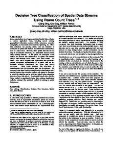
Figure 1 (left) shows the cost/accuracy tradeoff for the gcc benchmark. As a baseline, the cost of the trees built using the two best existing methods (as quantified in section 3) are also plotted. This curve is generated using five-fold cross validation to estimate the classification accuracy of the cost-sensitive decision tree for various values of γ. Among this set of (cost, accuracy) pairs, pareto optimal points are identified to generate the cost/accuracy curve. Since the absolute overhead slowdown is a function of program running time (which varies greatly from benchmark to benchmark), the costs here are normalized by the total instrumentation slowdown incurred if all available features were

0

10

CSGain −1

10

Benchmark Baseline CSGain w/FC, CTP mpg321 19.4% 158.3× gcc 24.2% 1.8× gzprintf 20.1% 1.7× latex 44.0% 468.1× foxpro 3.7% 1, 485, 943.7× lynx 1.9% 552.3× apache 8.9% 4, 684.2×

Mitchell Nunez

−2

Cost

10

−3

10

−4

10

−5

10

−6

10

70

75

80

85

90

95

Accuracy

Fig. 1. Left: cost/accuracy tradeoff for the gcc benchmark. Right: costs for six benchmarks with accuracy reductions of at most 1%. The Baseline column gives the decision tree cost when built with the baseline C4.5 algorithm, using CTP, expressed as a percentage of the total cost of instrumenting all features. The remaining columns provide the speedup ratio (defined as baseline cost / cost) for C4.5 using the cost-sensitive gain criteria (CSGain) with FC and CTP features.

instrumented. For example, a cost of .1 corresponds to instrumenting an average of 10% of all function calls in an execution of a program. Table 1 (right) gives decision tree costs for several benchmarks when trained using the baseline, cost-insensitive C4.5 algorithm (using FC and CTP behavior profiles), and also when trained using C4.5 with the CSGain criteria (4). This improvement is measured as the cost of the tree divided by the cost of the baseline, cost-insensitive tree (note that this is the inverse of the cost ratio term used in section 3). For the costsensitive algorithms, results are given for trees with accuracy levels that are no less than 1% lower than the cross validated accuracy of the baseline cost-insensitive classifier trained with FC and CTP representation. Our cost-sensitive algorithm yields reduction in execution of instrumentation points of up to six orders of magnitude.

5 Related work Building classifiers that minimize testing costs has received much attention in the field of medical diagnosis. However, the problem of medical diagnosis is fundamentally different from the forensic classification problem. Several cost-sensitive algorithms have been proposed that build decision trees using non-incremental methods, such as a genetic algorithm [14] and a “look ahead” heuristic [11]. These methods are not considered here, as the training time required is several orders of magnitude larger than a C4.5 based incremental algorithm. In this paper, we have focused on the problem of minimizing test cost while maximizing accuracy. In some settings, it is more appropriate to minimize misclassification costs instead of maximizing accuracy. For the two class problem, Elkan [6] gives a method to minimize misclassification costs given classification probability estimates. Bradford et al. compare pruning algorithms to minimize misclassification costs [1]. As both of these methods act independently of the decision tree growing process, they can be incorporated with our algorithms (although we leave this as future work). Ling et.

al. propose a cost-sensitive decision tree algorithm that optimizes both accuracy and cost. However, the cost insensitive version of their algorithm (i.e. the algorithm run if all feature costs are zero), reduces to a splitting criteria that maximizes accuracy, which is well known to be inferior to the information gain and gain ratio criterion [13, 10]. Integrating machine learning with program understanding is an active area of current research. Systems that analyze root cause errors in distributed systems [3] and systems that find bugs using dynamic predicates [2, 8, 9] may both benefit from costsensitive learning to decrease overhead monitoring costs.

6 Conclusion We have introduced two algorithms for the problem of minimizing feature costs for forensic classification. Our algorithms are modifications to the C4.5 decision tree algorithm that use a well motivated cost-sensitive splitting criteria. We provide extensive experiments on real data and objectively demonstrate that our criterion yield algorithms that build cheaper trees than existing methods. Finally, we implement our method in a novel cost-sensitive forensic classification problem, the C LARIFY system. We show our algorithm can reduce overhead costs by many orders of magnitude at only a slight (< 1%) reduction in classification accuracy.

References 1. J. Bradford, C. Kunz, R. Kohavi, C. Brunk, and C. Brodley. Pruning decision trees with misclassification costs. In European Conference on Machine Learning, 1998. 2. Y. Brun and M. D. Ernst. Finding latent code errors via machine learning over program executions. In ICSE, 2004. 3. I. Cohen, S. Zhang, M. Goldszmidt, J. Symons, T. Kelly, and A. Fox. Capturing, indexing, clustering, and retrieving system history. In SOSP, 2005. 4. T. M. Cover and J. A. Thomas. Elements of information theory. Wiley Series in Telecommunications, 1991. 5. C.L. Blake D.J. Newman, S. Hettich and C.J. Merz. UCI repository of machine learning databases, 1998. 6. C. Elkan. The foundations of cost-sensitive learning. In International joint conference on artifical intelligence, 2001. 7. J. Ha, H. Ramadan, J. Davis, C. Rossbach, I. Roy, and E. Witchel. Navel: Automating software support by classifying program behavior. Technical Report TR-06-11, University of Texas at Austin, 2006. 8. S. Hangal and M. S. Lam. Tracking down software bugs using automatic anomaly detection. In ICSE, 2002. 9. B. Liblit, M. Naik, A. X. Zheng, A. Aiken, and M. I. Jordan. Scalable statistical bug isolation. In PLDI, 2005. 10. T. Mitchell. Machine Learning. WCB McGraw-Hill, 1997. 11. S.W. Norton. Generating better decision trees. In International joint conference on artifical intelligence, 1989. 12. M. Nunez. The use of background knowledge in decision tree induction. In Machine Learning, 1991. 13. R. Quinlan. C4.5: programs for machine learning. Morgan Kaufmann Publishers, 1992. 14. P. Turney. Cost-sensitive classification: Empirical evaluation of a hybrid genetic decision tree induction algorithm. In Journal of artificial intelligence research, 1995.