Creating Compact Architectural Models by Geo-registering Image Collections Radek Grzeszczuk Nokia Research Center
Jana Koˇsecka George Mason University
Ramakrishna Vedantham Nokia Research Center
[email protected]
[email protected]
[email protected]
Harlan Hile University of Washington
[email protected]
Abstract We present a method for automatically constructing compact, photo-realistic architectural 3D models. This method uses simple 3D building outlines obtained from existing GIS databases to bootstrap reconstruction and works with both structured and unstructured image datasets. We propose an optimal view-selection algorithm for selecting a small set of views for texture mapping that best describe the structure, while minimizing warping and stitching artifacts, and producing a consistent visual representation. The proposed method is fully automatic and can process large structured datasets in close to real-time, making it suitable for large scale urban modeling and 3D map construction.
1. Introduction 3D modeling of urban areas is entering a phase of rapid development driven by cheaper sensors, better algorithms and enhanced computational capabilities. This enables new navigation systems with more immersive, easier-to-follow instructions. The scale of modeling required by such applications necessitates algorithms that are fast. The profusion of mobile networked devices with restricted computing power and bandwidth, such as cell phones and PDAs, also suggests that these models should be compact and efficient. In this work we present a novel, fully-automated pipeline for constructing compact 3D models. The method works both with structured image datasets (characterized by a large number of sequential views) and with unstructured image datasets (such as those found on popular photo sharing sites). For the structured image datasets, which typically come from surveying vehicles equipped with precise sensor for accurately registering camera poses, our modeling pipeline can produce high-quality 3D models very fast— processing hundreds of images per second. A key component of our approach is to leverage building outlines (footprint and height) obtained from existing Geographic Information System (GIS) databases to register unstructured photo collections with the building, perform view selection, and to synthesize a 3D model. In our fully
automatic 3D reconstruction pipeline, we developed a robust geo-registration technique for the unstructured image collections. We propose a novel, optimal view-selection algorithm, which from a large number of views can select a small subset that best describes the structure, while minimizing warping and stitching artifacts. From the selected views, we automatically synthesize a compact 3D model of high quality that we can easily re-target to devices with a broad range of computational and bandwidth capabilities. The dominant existing approach to modeling uses highly structured data collected by cameras mounted on a driving vehicle equipped with inertial GPS sensors [15] and augmented with 3D LiDaR data [9, 25]. The resulting models tend to have visual artifacts (holes, local deformations) due to difficulties during the dense reconstruction stage. Cornelis et al. [4] use a highly-optimized 3D reconstruction pipeline that can run close to real-time by assuming that the building facades can be approximated with surfaces ruled in the vertical direction. They extend the reconstruction framework by integrating it with a car detection and localization module that instantiates virtual placeholder models to cover parts of the facades that have missing data. Alternative approaches use unstructured photo collections [19]. Instead of creating 3D models, they focus on novel ways to explore and navigate the image collections [18]. Several approaches use human assistance in the modeling stage. A pioneering example is the work of Debevec et al. [5], where a human instantiates a simple geometric primitive and manually selects a small number of carefully calibrated views to texture map the model. Werner and Zisserman [23] propose an automated technique that achieves similar results. Dick et al. [6] utilize prior knowledge about architecture to reconstruct the geometry. More recent examples include [17, 24]. The approach we present here uses building extents and automated geo-registration and is applicable to urban areas for both structured and unstructured image collections. The buildings in GIS databases are typically represented as sets of extruded and stacked polygons each with associated height. Our approach to create visually pleasing 3D models for these types of urban structures complements the existing
Figure 1. Examples of 3D reconstructions automatically obtained using the presented technique from unstructured photo collections.
modeling pipelines and produces models of lower complexity and superior quality. Examples using our approach are shown in Figure 1. Contributions. The main contributions of this work are: • A novel robust geo-registration technique for unstructured image collections: the images and sparse 3D reconstructions are registered to a map and a building outline using noisy GPS data; • A new efficient and optimal view-selection algorithm which distills a large number of images down to a small subset of views that best describe the structure while minimizing warping and stitching artifacts; • Final creation of compact, photo-realistic 3D models utilizing selected images for texture mapping. These models are of superior visual quality and use a simple representation amenable to real-time rendering on a broad range of devices.
1.1. Related Work The relevant work on 3D modeling from images was mentioned in the introduction. Here, we focus on the review of work related to geo-registration and view-selection. With the advances in scale-invariant feature matching and robust motion estimation, the problem of registering multiple views of the same landmark from unstructured image sets has become feasible. In the absence of GPS coordinates and viewing direction information, the process of registering 3D reconstructions with a map has been done manually [19]. Early systems [13] tried to integrate the constraints from GPS measurements with pose estimation by manually establishing the correspondences between the image features and the points in the world coordinate system. In contrast, we propose to automatically geo-register unstructured image collections despite sparse and noisy GPS tags. Structured image collections from full-fledged model acquisition platforms are typically accurately geo-registered because GPS measurements are integrated with additional inertial and odometry measurements, yielding quality camera pose estimates in the world coordinate system without additional alignment.
Work on view selection for sensor placement has received much attention in the robotics community in the context of model building and exploration of 2D environments. Authors in [10] formulated the coverage problem as a set cover problem and obtained approximate solutions either by relaxation or greedy algorithms, while considering range and grazing angle/incidence constraints. In the graphics community alternative measures of the view quality have been proposed which implicitly included the number of visible polygons. In [21], the authors tackled the problem in 3D and proposed a solution using a greedy technique. In image-based rendering using multi-view panoramas, the authors in [1] addressed the view selection problem by using a Markov Random Field framework to select the best viewpoint for each pixel of the output image. In this work, we show how to efficiently select a subset of views that completely cover the visible area and is optimal in terms of a predefined view quality metric. This is done by reducing the view selection problem to a task scheduling problem, which can be solved in polynomial time using minimal cost flow algorithm [2]. Overview. Figure 2 shows the block diagram of our 3D reconstruction pipeline. The method for unstructured photo collections first registers the views and then robustly aligns them to the world map. Efficient view selection and imagebased model synthesis stages are the same for both types of input data. From the diagram, we see where the landmark/building outline is used as an input to the algorithm. We start by describing preliminaries, such as sources of image data and image data organization. Section 2.1 describes the method for robustly aligning the results of 3D structure-from-motion recovery to the map. Section 2.2 describes the optimal view selection algorithm. Finally, Section 2.3 describes the process of automatically creating an image-based model of the landmark from the selected views.
2. 3D Reconstruction Pipeline Image Datasets. In this work, we focus on supporting both structured and unstructured image collections. We use two
Unstructured Image Set
Structure From Motion
Structured Image Set
Robust Map Alignment
Select Building Views
Efficient View Selection
Building Outline
Image‐Based Model Synthesis 3D Model of Landmark
Figure 2. Block diagram of automatic creation of compact architectural models. The algorithm supports two paths—one for the unstructured photo collections and one for structured image datasets. Light green boxes indicate the input to our algorithm.
source of unstructured image data. One is a database of landmarks and images from an existing outdoor augmented reality project [20]. The database contains images contributed from many users taking pictures with GPS-enabled camera phones and selecting a label for each image from a list of nearby landmarks. This database also contains building extent and height information for the landmarks acquired from an existing GIS database. Our other source of unstructured data is the online geo-tagged photo sharing service Panoramio. For these reconstructions, we manually traced the building outline on the satellite image rather than mining the appropriate GIS database. Both of these data sources have high GPS error which our robust alignment algorithm is able to handle. We also ran experiments on two types of structured data. The Baity-Hill dataset from UNC-Chapel Hill [15] is densely captured at 30 fps with a camera rig mounted on a driving vehicle. It contains on the order of 1300-1500 images per building. The images have a fairly narrow field of view so in order to cover the whole building facade multiple views are needed in the vertical direction. Earthmine Inc. (www.earthmine.com) provides structured dataset of omni-directional panoramic images. We calculated which portions of these panoramas contained the building of interest and extracted multiple views with a fixed field of view of 60o , producing on the order 100-300 images per building.
2.1. Robust Map Alignment The first step for processing the unstructured photo collections is to compute full 3D registration using large scale wide-baseline matching and a structure-from-motion (SfM) estimation algorithm. In this stage we use an open source package developed at University of Washington by Snavely et al. [19] which facilitates fully automatic matching and full 3D registration of overlapping views using SIFT features and bundle adjustment 1 . RANSAC Alignment. Given the set of registered images, where a subset of them is tagged by GPS locations, we automatically estimate the similarity transformation between the two sets of measurements. Since there is no initial guess of the transformation or reliable point correspondences, we estimate the alignment by following two step strategy. In 1 See
http://phototour.cs.washington.edu/bundler.
the first stage we estimate initial alignment using the correspondences between centers of projections coordinates (reconstructed camera positions) and their associated GPS coordinates using a RANSAC algorithm with automatic scale selection [22]. We estimate an alignment from two reconstructed camera locations Ci = [Xi , Zi ] and Cj = [Xj , Zj ] and two GPS coordinates extracted from the image tags and transformed to the UTM coordinates Ui = [Ei , Ni ] and Uj = [Ej , Nj ]. The scale s is the ratio of the two distances kU −U k s = kCii −Cjj k . The translation t is the displacement vector t = Ui − Ci . The rotation matrix R describes the 2D rotation between the lines connecting the reconstructed image locations Ci and Cj and the corresponding reference GPS locations after the translation alignment Ui + t and Uj + t. These hypotheses are generated by randomly sampling pairs of poses whose distance is above some threshold (2m in our case). For each hypothesis Tk = (Rk , tk , sk ) we transform all reconstructed camera poses to obtain their GPS positions and then compute the residual alignment error of all the remaining poses. The hypothesis with the largest number of inliers is chosen as the best one. Inlier/outlier classification is done based on the threshold of the residual errors. Since the GPS errors vary based on the location, we estimate this threshold from the histogram of the residuals computed over a large number of hypotheses using automated scale selection techniques. Note that only a small fraction of the images needs to have GSP data— typically about 10% of images. For very noisy data sources, such as Panoramio, this ratio goes up to 30%. The RANSAC step approximately aligns the 3D reconstruction with the map data. For the unstructured image collections, characterized by noisy GPS coordinates, this step does most of the work. In the next stage we refine this result by aligning the 3D reconstruction to the building outline. ICP Alignment. We project the 3D reconstruction to the ground plane and then match the points to the building outline using an Iterative Closest Point (ICP) technique. In our experience the quality of the 3D reconstructions produced by the SfM algorithm matches well with the fidelity of the GIS building outlines. If more detailed point clouds were available, we might be able refine the building outlines to better fit the data.
Figure 3. The top row shows alignment of the 3D reconstruction points projected on the ground plane after the initial RANSAC alignment (cyan) and after final ICP alignment (yellow). In addition to good alignment, all the outlier points have been removed. The bottom row shows the camera poses (green dots are original GPS readings connected by a line to the corresponding red dots indicating computed camera locations; yellow lines indicate viewing directions) and the aligned reconstruction points. The red contours show building outlines.
We use a robust version of the algorithm proposed by [3] adopted for similarity transformations in 2D. In particular we seek such a similarity transform T = (R, t, s) so as to minimize the errors between and the PN reconstructed points 2 ks(Rp + t − q ¯ )k where pi building outline: e = i i=1 are projections of 3D reconstructed points and q¯i ’s are the closest points to each pi which are along the line perpendicular to the nearest boundary. This non-linear objective function is linearized assuming sin θ ≈ θ and can be solved using linear least squares. Several (on average 3) iterations are carried out until the error reaches an equilibrium point. The outliers are rejected by removing all the points whose distance to the closest boundary d > 3 mediani (di ) which naturally adjusts the threshold in subsequent iterations. Figure 3 shows the result of two stages of the alignment algorithm for 3 different buildings; The top images compare the initial RANSAC alignment and the ICP alignment. The bottom images show the final results compared to the initial GPS input. It is worth noting that some of the GPS locations read from image tags have high error (green dots showing on top of a building and in the middle of a street). An additional challenging example is shown in Figure 7.
2.2. Optimal View Selection The goal of this next step is to find a set of images describing the visible portions of a building completely and
accurately so that we can produce a texture mapping of our simplified model. We maximize the quality of the reconstruction by ranking the images based on how well they represent the portion of the building that they see, and we ensure the optimality by efficiently computing a view selection that best covers the visible portions of the building using the highest ranked images. Our task is closely related to the problem of sensor placement studied extensively in the robotics, computer vision and graphics communities [7, 16]. In [10], the authors formulated the view selection as a set cover problem, which is NP-hard, and solved it approximately using a greedy algorithm. A novel insight into solving this problem efficiently comes from imposing a view ordering induced by the parametrization of the building surface and exploiting the visibility relations between the views. This allows us to transform the above stated problem into a scheduling task [8] for which an efficient combinatorial optimization solution exists that solves it using minimal cost flow algorithm [2]. We first outline the view selection algorithm in general terms and then describe the implementation specific details. Let’s assume we have a set of views C = {c1 , c2 , . . . , cn } that have been ranked, i.e., each view ci ∈ C has been given a weight wi reflecting its quality. A scheduling task oper-
S (θ , φ ) 0.2
0.3
2
0.4 0.3
1
S 1
4
2
1
2
3
4
5
0.3
0.2
0.4
0.3
0.2
0.3
0.2
0.0
0.3
0.2
0.0
0.2
3
3
0.2 5
4 5
0.0 0.2
S vfi
T
ci
Qvfi Fvfi
0.0 0.0
Figure 4. View selection for a simple 3D surface covered by 5 views. The number in the bottom-left corner of a view specifies its ordering. The number in the center of a view indicates its weight. The corresponding DAG with highlighted edges along the longest path from source node S to target node T is shown on the right.
ates on a set of jobs with start and end times, so we need to provide an analogous ordering of our views. Any ordering, as long as it consistently represents the overlap relationship between the views, will suffice. We define ours by traversing a building outline in the bottom-up left-right order. Figure 4 (left) shows a result of such ordering for a simple case of 5 overlapping views. Once we established an ordering, we determine the overlap relations between views by checking which of them see overlapping portions of the building outline as explained below in the next subsection. Next, we follow the DAG construction presented in [2]. For each view ci ∈ C create a node i. Add an edge between i and j for each view cj that does not intersect ci and such that tj ≥ ti , where t describes the view ordering. Assign the edge a value of wj . Add a source node S and connect it to each node i with weight wi . Add a sink node T and connect it to each node i with weight 0. The solution that gives an optimal view selection with the best coverage of visible areas is obtained by performing a topological sort of the DAG and computing the longest path in the DAG using Dijkstra’s algorithm. Refer to Figure 4 (right) for an example. Visibility Computation. We assume that a building outline is composed of a set of 2D polygons describing its footprint and each is given a fixed height2 . First, we divide each 2D polygon of the building footprint into a sequence of segments S = {s1 , s2 , . . . , sl }. Next we vertically extrude each segment sj ∈ S into a rectangle Qj with height hj and divide it into a set of small facets Fj = {fj1 , fj2 , . . . , fjh }. The segment size is selected for adequate quantization of view selection based on the average distance of the cameras from the building outline. Typically, this results in a segment size in the range of 2-4 meters. The facet height is set to be equal to the segment size. Next, a 2D visibility polygon, which properly solves for planar occlusions, is computed for each camera ci using the library for visibility computation provided by [14]. We find 2 Currently we are solving a simplified 3D visibility problem that is suitable for our building models and we leave an implementation of the full 3D visibility computation as future work.
Figure 5. Right: the selection of visible segments. Left: the selection of visible facets. i the segments Svf ∈ S that are inside the visibility polygon and the viewing frustum of camera ci . The facets corresponding to the rectangles Qivf are then projected into the image of camera ci to determine which of them are visible. i We refer to the set of visible facets as Fvf . See Figure 5 for an illustration. The set of visible facets becomes the basis of computing view overlaps, explained below. Whenever there is an occlusion boundary present in the sequence of visible segments, we break up the view of camera ci into multiple views along the occlusion boundary. i i of high quality visi∈ Fvf Finally we form a subset Fhq ble facets that meet the incidence and range constraints. The range constraint states that the distance from the camera loi cation ci to the center of facet fk ∈ Fhq must be within an acceptable range: dm ≤ d(ci , fk ) ≤ dM . The incidence constraint states that the angle between the normal of fk and the direction from the center of fk to camera location ci is less than a certain angle αM . For unordered image collections we specify these distance constraints in terms of the average distance computed across all cameras and all visible polygons, typically setting dm to be one third this distance and dM to be three times this distance. We set the incidence angle threshold to αM = 75o .
High-quality visible facets are used to determine which views are non-overlapping. We mark two views i and j as i non-overlapping if they have no facets in common (Fhq ∩ j Fhq = ∅). These overlap relations are then used to build the DAG as explained in the previous subsection. (An edge is added to the graph for each non-overlapping pair of views.) View Ranking. The view quality wi of camera ci is computed as a product of three terms. The first term favors images that are facing the building directly and is defined as the average dot product between the normals of the visible facets and the viewing direction from the camera location ci to centers of the facets. The second term is the portion of the i view occupied by the visible facets Fhq , meaning the building covers most of the field of view. Finally, the third term is the portion of the total number of facets that they represent, so the image contains a large portion of the building. This ranking naturally leads to selection of a small number of images that minimize warping and stitching artifacts.
Figure 6. Selected views for 3 landmarks from an unstructured dataset. Red dots indicate the center of projection of the cameras, the magenta triangles indicate the field of view of the camera, and the yellow lines emanate form the centers of projection to the centers of good segments of a given view (shown as green triangles).
Overlap Regions. The scheduling problem is not allowed to overlap jobs, resulting in the gaps in the final solution. In order to avoid gaps left between the selected views, we narrow the field of view of each camera by a fixed-size overlap region. The amount of overlap is measured in segments. If the overlap is set to one, we simply remove the outermost i ring of facets from Fhq . If the overlap is set to two, we remove the two outermost rings, and so on. Typically we never use an overlap region of size more than three segments. We recompute the overlap relations between the views and run the view selection algorithm multiple times, once for each size of the overlap region, and select the result that gives us the highest score solution (measured as a sum of qualities of visible facets) without any gaps. In case gaps do remain, the overlap regions are used to fill in the gaps between the selected views. The image with the highest quality view of the gap is selected to fill it. View Selection Results. Figure 6 shows the results of the view selection algorithm applied to 3 examples taken from our unstructured dataset. As we see, in each case the algorithm selected a small number of good quality views that completely cover the visible areas of the building. The corresponding 3D reconstructions are shown in Figure 1. Figure 7 shows the result of the alignment, view selection and 3D model synthesis applied to an unstructured photo collection from Panoramio. The alignment step worked robustly despite a large number of outliers with very high GPS error. As in the previous case, we get a small number of high quality views that completely describe the visible portion of the structure. A rough outline of the Colosseum was entered manually from a satellite image. Figure 8 (left image) shows 347 views of the Ferry Building in San Francisco extracted from the Earthmine database. We show a green dot for each camera location and a yellow line for the corresponding viewing direction.
The right image shows the 16 views automatically selected for this landmark. The 3 far away views see the tall clock tower, while the remaining 13 close views cover the building itself. In this case the visibility was computed separately for the building and for the tower, but the view selection was done in a single step. The building outline for this landmark was extracted from the Navteq’s NavStreets database. For the Baity Hill dataset we had 1200 views corresponding to the reconstructed building—600 for the bottom and 600 for the top part of the building. We have constructed a single DAG out of all views (after adding an overlap region, the top and bottom views were non-intersecting) and automatically computed 30 views that completely cover the visible portion of the building. Figure 9 (left image) shows the selected view for the top half of the building (the views selected for the bottom part look very similar). The right image show a view generated with the synthesized 3D model. Since the building outline information for this landmark did not exist in the available GIS databases, we manually traced it in a satellite image. Low accuracy of the resulting building outline is the cause of the misalignment artifacts visible in the synthesized view. In each of the presented examples, the view selection and the 3D model synthesis took less than 10 seconds of computation on a commodity CPU.
2.3. Image-Based Model Synthesis Since our algorithm builds models out of large, contiguous views that introduce minimal stitching and warping artifacts, we do not have to perform a lot of post-processing to improve their appearance. However, one problem with the unstructured image datasets is a large variation in colors and exposures of the images they contain. Currently, we offer only a simple improvement: we modify the colors of selected views by adjusting the means and standard
Figure 7. 3D reconstruction from Panoramio data. The left image illustrates the alignment of the reconstruction to the building outline (only a subset of reconstructed points and cameras is shown). Note very high error indicated by red line connecting red dots (reconstructed pose) and green dots (image GPS tag). The center image shows the selected views. The right image shows the reconstructed model.
Figure 8. Left image shows 347 views for the Ferry Building in San Francisco extracted from the Earthmine Inc. database. Right image shows a subset of 16 views that were selected to represent that landmark.
deviations of each color channel separately, as described in [16], to make them match the overall mean and standard deviation of the image collection. Other techniques used in panorama stitching such as graph-cut and Poisson blending could also be applied to provide smoother transitions. In the future, we plan to look at approaches that incorporate a color similarity metric directly into the view selection process. Our models can be represented very succinctly. They consist of approximately 1000 rectangles, 10-20 images and the associated texture coordinates; in most cases this is several orders of magnitude less images than the original image set. Additionally they are easily amenable to different resolution displays. The only thing needed to change the level of detail of the models is to downsample images. For example, when targeting a display of resolution 1024x768, we use JPEG compressed images of resolution 0.25 Mpix for a total model size of 200-400KB. When targeting a display of resolution 640x480, we use images of 50 Kpix for a total size of 50-100KB, which is reasonable for mobile devices. Given relatively high quality of the reconstructions,
we feel this is a significant accomplishment that will allow such models to be proliferated to a wide range of devices and used ubiquitously. Naturally, much more can be done to further improve the quality of our models. For example, objects in the environment that often occlude buildings, such as cars and trees, can lead to visually unpleasant artifacts when projected onto the simplified geometry. These objects are important to human recognition of a building, even in a low accuracy representation. In the future, we plan to use object detection methods to instantiate virtual placeholder models as in [4]. This modification to our modeling pipeline should enhance the visual realism of the resulting scene while maintaining real-time performance. Image-based procedural modeling [12] offers a promising approach for further enhancing model quality. It is also worth noting that our models lack roofs and may have additional artifacts due to the inaccurate skyline determination. The roofs are generally not a problem because most street-level photography includes little view of the roof and newly synthesized street-level views still look reasonable if any roof present is mapped onto the plane of the building. If roofs are desired, flat roof geometry can be added from satellite data, or more complex methods can produce a detailed roof structure [11].
3. Conclusion We have presented a novel, fully-automated pipeline for constructing compact 3D architectural models for both structured and unstructured image datasets. By leveraging building outlines and formulating view selection as a scheduling problem, we are able to produce high quality, compact texture mapped models in near real time. These models are orders of magnitude smaller than the original input data, and are suitable for use on a variety of platforms.
Figure 9. The left image shows the views selected for the top portion of a building from the Baity Hill dataset (the views selected for the bottom part look very similar). The right images shows a view generated with the synthesized 3D model.
References [1] A. Agarwala, M. Agrawala, M. Cohen, D. Salesin, and R. Szeliski. Photographing long scenes with multi-viewpoint panoramas. In SIGGRAPH, 2007. 2 [2] E. M. Arkin and E. B. Silverberg. Scheduling Jobs with Fixed Start and End Times. Discrete Applied Mathematics, 18(1):1–8, 1987. 2, 4, 5 [3] Y. Chen and G. Medioni. Object Modelling by Registration of Multiple Range Images. In IEEE ICRA, pages 2724–2729, 1991. 4 [4] N. Cornelis, B. Leibe, K. Cornelis, and L. V. Gool. 3D Urban Scene Modeling Integrating Recognition and Reconstruction. Int. J. Comput. Vision, 78(2-3):121–141, 2008. 1, 7 [5] P. E. Debevec, C. J. Taylor, and J. Malik. Modeling and Rendering Architecture from Photographs: a Hybrid Geometryand Image-Based Approach. In SIGGRAPH ’96, pages 11– 20, New York, NY, USA, 1996. ACM. 1 [6] A. R. Dick, P. H. S. Torr, and R. Cipolla. Modelling and Interpretation of Architecture from Several Images. Int. J. Comput. Vision, 60(2):111–134, 2004. 1 [7] U. M. Erdem and S. Sclaroff. Automated Camera Layout to Satisfy Task-Specific and Floor Plan-Specific Coverage Requirements. Compututer Vision and Image Understanding, 103(3):156–169, 2006. 4 [8] T. Erlebach and F. C. R. Spieksma. Interval Selection: Applications, Algorithms, and Lower Bounds. Journal of Algorithms, 46(1):27–53, 2003. 4 [9] C. Frueh, S. Jain, and A. Zakhor. Data Processing Algorithms for Generating Textured 3D Building Facade Meshes from Laser Scans and Camera Images. Int. J. Comput. Vision, 61(2):159–184, 2005. 1 [10] H. Gonz´alez-Banos and J.-C. Latombe. A Randomized ArtGallery Algorithm for Sensor Placement. In SCG ’01: Symposium on Computational Geometry, pages 232–240, New York, NY, USA, 2001. ACM. 2, 4 [11] P. M¨uller, P. Wonka, S. Haegler, A. Ulmer, and L. Van Gool. Procedural Modeling of Buildings. ACM Trans. Graph., 25(3):614–623, 2006. 7 [12] P. M¨uller, G. Zeng, P. Wonka, and L. Van Gool. Imagebased Procedural Modeling of Facades. ACM Trans. Graph., 26(3):85, 2007. 7
[13] T. K. Ng and T. Kanade. PALM: Portable Sensor-Augmented Vision System for Large-Scene Modeling. In 3DIM, pages 473–482, 1999. 2 [14] K. J. Obermeyer. The VisiLibity Library: A C++ Library for Floating-Point Visibility Computations. Available from http://www.VisiLibity.org, 2008. R-1. 5 [15] M. Pollefeys and et. al. Detailed Real-Time Urban 3D Reconstruction from Video. International Journal of Computer Vision, 78, 2008. 1, 3 [16] E. Reinhard, M. Ashikhmin, B. Gooch, and P. Shirley. Color Transfer between Images. In IEEE Computer Graphics and Applications, volume 21, pages 34–41, 2001. 4, 7 [17] S. N. Sinha, D. Steedly, R. Szeliski, M. Agrawala, and M. Pollefeys. Interactive 3D Architectural Modeling from Unordered Photo Collections. ACM Trans. Graph., 27(5):1– 10, 2008. 1 [18] N. Snavely, R. Garg, S. Seitz, and R. Szeliski. Finding Paths through the World’s Photos. In SIGGRAPH, 2008. 1 [19] N. Snavely, S. M. Seitz, and R. Szeliski. Photo Tourism: Exploring Photo Collections in 3D. In SIGGRAPH ’06, pages 835–846, New York, NY, USA, 2006. ACM. 1, 2, 3 [20] G. Takacs and et. al. Outdoors Augmented Reality on Mobile Phone using Loxel-Based Visual Feature Organization. In Proceeding of the 1st ACM International Conference on Multimedia Information Retrieval, pages 427–434, 2008. 3 [21] P.-P. V´azquez, M. Feixas, M. Sbert, and W. Heidrich. Automatic View Selection Using Viewpoint Entropy and its Application to Image-Based Modelling. Computer Graphics Forum, 22(4):689–700, Nov. 2004. 2 [22] H. Wang and D. Sutter. Robust fitting by adaptive-scale residual consensus. In ECCV, volume 3023, pages 107–118, 2001. 3 [23] T. Werner and A. Zisserman. New Techniques for Automated Architectural Reconstruction from Photographs. In ECCV ’02: Proceedings of the 7th European Conference on Computer Vision-Part II, pages 541–555, 2002. 1 [24] J. Xiao, T. Fang, P. Tan, P. Zhao, E. Ofek, and L. Quan. Image-Based Fac¸ade Modeling. ACM Trans. Graph., 27(5):1–10, 2008. 1 [25] Q.-Y. Zhou and U. Neumann. Fast and Extensible Building Modeling from Airborne LiDAR Data. In GIS ’08: ACM SIGSPATIAL Conf. on Advances in Geographic Information Systems, pages 1–8, New York, NY, USA, 2008. ACM. 1